A Markov Chain Based Method for Generating Long-Range Dependence

Abstract

This paper describes a model for generating time series which exhibit the statistical phenomenon known as long-range dependence (LRD). A Markov Modulated Process based upon an infinite Markov chain is described. The work described is motivated by applications in telecommunications where LRD is a known property of time-series measured on the internet. The process can generate a time series exhibiting LRD with known parameters and is particularly suitable for modelling internet traffic since the time series is in terms of ones and zeros which can be interpreted as data packets and inter-packet gaps. The method is extremely simple computationally and analytically and could prove more tractable than other methods described in the literature.

I Introduction

Long-range dependence (LRD) is a statistical phenomenon which is used to describe a process which exhibits significant correlations even between widely separated points. A more formal definition is given in the next part of this paper. Roughly speaking, a process with a high degree of LRD can be thought of as correlated at all scales. A good introduction to the topic of LRD is provided by Beran (1994) and a discussion in the context of telecommunications traffic is given by Clegg (2004). LRD is most often characterised by the Hurst parameter, $H$, which is in the range $(1/2,1)$ for a time series which exhibits LRD. If $H=1/2$ then this indicates the data is independent or has only short-range correlations. The topic of LRD has attracted a great deal of interest since LRD has been observed in time series measured in fields as diverse as finance, internet traffic and hydrology.

This paper introduces and tests a mechanism for generating LRD based on an infinite Markov chain. The traffic stream generated is binary in nature and the model has only two parameters, the mean and the Hurst parameter of the generated traffic. This section provides a brief introduction to the topic of LRD in the context of telecommunications networks and discusses currently used generation mechanisms for modelling LRD and also methods which are currently used to measure LRD in a time series. Section II describes the infinite Markov model. In Section III it is proved that the model does in fact generate a time series with a given mean and with LRD having a given Hurst parameter. Finally, Section IV tests the model against other standard LRD generation models and discusses the advantages of the model.

I.1 A Brief Introduction to LRD

A number of different (and not necessarily equivalent) definitions of LRD are in use in the literature. A commonly used definition is the one given here.

Definition 1.

A weakly stationary time series exhibits LRD if the absolute value of its autocorrelation function (ACF) $\rho(k)$ does not have a finite sum. That is,

$$\sum_{k=-\infty}^{\infty}|\rho(k)|=\infty.$$

It is often assumed that the ACF has the specific asymptotic form,

$$\rho(k)\sim c_{\rho}k^{-\alpha},$$ (1)

for some positive constant $c_{\rho}$ and some real $\alpha\in(0,1)$. Note that this is equivalent to a functional form for the spectral density $f(\lambda)$ defined by,

$$f(\lambda)=\frac{\sigma^{2}}{2\pi}\sum_{k=-\infty}^{\infty}\rho(k)e^{ik\lambda}.$$

Equation (1) is equivalent to,

$$f(\lambda)\sim c_{f}|\lambda|^{-\beta},$$

as $\lambda\rightarrow 0$, where $\sigma^{2}$ is the variance, $c_{f}$ is some positive constant and $\beta\in(0,1)$. The Hurst parameter is then given by $H=(1+\beta)/2$.

It should be noted that here, and throughout this paper, $f(x)\sim g(x)$ is used to mean $f(x)/g(x)\rightarrow 1$ as $x\rightarrow\infty$ — sometimes, in the literature, the symbol is used to mean asymptotically proportional to or $f(x)/g(x)\rightarrow k$ for some constant $k$ as $x\rightarrow\infty$.

The constant $\alpha$ in (1) is sometimes expressed in terms of the Hurst parameter $H=1-\alpha/2$. The Hurst parameter as defined by this relation and (1) is the most commonly used measure of LRD in the telecommuncations literature.

The reason for the interest in the subject within the field of telecommunications is the fact that LRD has been observed in various time series related to internet traffic Leland et al. (1993); Willinger et al. (1997); Morris and Lin (2000). It is widely recognised that the engineering implications of LRD on queuing performance can be considerable. If Internet traffic is not modelled well by independent or short-range dependent models then much traditional queuing theory work based upon the assumption of Poisson processes is no longer appropriate. Traffic which is long-range dependent in nature can have a queuing performance which is significantly worse than Poisson traffic. Modelling has shown how phase transitions can arise in computer networks Ohira and Sawatari (1998), how and this phase transition can be related to LRD Valverde and Sole (2001); Woolf et al. (2002).

In general it has been found that a higher Hurst parameter often increases delays in a network, increases the probability of packet loss and affects a number of measures of engineering importance. In fact Erramilli et al. (1996) claims that the Hurst parameter is “…a dominant characteristic for a number of packet traffic engineering problems…”. Some of the effects on queuing performance are given by Norros (1994); Sahinoglu and Tekinay (1999). However, Neidhardt and Wang (1998) shows that while the Hurst parameter is important to queueing, the relationship is not a simple one — in some cases a high Hurst parameter may improve performance or have no effect. The issue of the scale and nature of the effect of LRD on queuing remains contentious.

I.2 Current Generation Mechanisms for LRD

A number of modelling techniques are currently used for generating traffic streams exhibiting LRD. Of these, the most commonly encountered in the telecommunications literature are Fractional Gaussian Noise processes (FGN), Fractional Auto-Regressive Integrated Moving Average models (FARIMA, also refered to as ARFIMA), iterated chaotic maps and wavelet modelling.

The FGN process is usually defined as increments of the Fractional Brownian Motion (FBM) process. An FBM process $B_{H}(t)$ is defined by:

$$\begin{split}\mathbb{P}\left[B_{H}(t+k)-B_{H}(t)\leq x\right]=\\ (2\pi)^{-\frac{1}{2}}k^{-H}\int\limits_{-\infty}^{x}\exp\left(\frac{-u^{2}}{2k^{2H}}\right)du,\end{split}$$

where $\mathbb{P}\left[X\right]$ is a probability of an event $X$ and $H\in(1/2,1)$ is the Hurst parameter. This can be seen as a generalisation of the more common Gaussian White Noise process. A number of authors have described methods for generating FGN and FBM Mandelbrot (1971), Davies and Harte (1987) and Paxson (1997).

The FARIMA model is an obvious modification of the traditional ARIMA$(p,d,q)$ model from time series analysis, allowing $d\in(-1/2,1/2)$ instead of $d\in\mathbb{Z}_{+}$. FARIMA processes were proposed by Granger and Joyeux (1980) and a description in the context of LRD can be found in (Beran, 1994, pages 59–66). As might be expected the $d$ parameter relates to the Hurst parameter. The relation is simply $H=d+1/2$ — note that this only produces legitimate values for $H$ when $d\in(0,1/2)$.

Iterated chaotic maps which exhibit intermittency are also commonly used to generate time series exhibiting LRD. Given a starting value $x_{0}\in(0,1)$ then a time series $\{x_{n}:n\in\mathbb{N}\}$ can be generated by the following map

$$x_{n+1}=\begin{cases}x_{n}+\frac{1-d}{d^{m_{1}}}x_{n}^{m_{1}},&0<x_{n}<d,\\ x_{n}-\frac{d}{(1-d)^{m_{2}}}(1-x_{n})^{m_{2}},&d<x_{n}<1,\end{cases}$$

where $d\in(0,1)$ and $m_{1},m_{2}\in(3/2,2)$. If $x_{0}\in(0,1)$ then $x_{n}\in(0,1)$ for all $n\in\mathbb{N}$. If this time series is used to generate a binary time series $\{y_{n}:n\in\mathbb{N}\}$ by the rule $y_{i}=0$ if $x_{i}<d$ and $y_{i}=1$ otherwise then the series can be shown to exhibit LRD with a Hurst parameter given by $H=(3m-4)/(2m-2)$. This map is illustrated in Figure 1. An explanation for the presence of LRD in this map is provided by examining the behaviour of the orbits at $x_{i}$ near zero or one. The escape from points near zero or one is extremely slow and this causes long sequences of zeros or ones in the generated $y_{i}$ series. Pioneering work in this area is Wang (1989) with early applications to telecommunications being given by Erramilli et al. (1995). This mechanism is particularly suited for generating data for modelling of packet networks since the ON ($y_{i}=1$) state can be considered to be a packet and the OFF ($y_{i}=0$) state as an interpacket gap.

Figure 1: Graph of a map which can be used to generate LRD.

In fact, the work described in Wang (1989) relates to the Markov chain based work described in this paper as it approximates the chaotic map approach as a piecewise linear map which can, in turn, be modelled as a Markov chain with the topology described later. A number of other papers have used Markov chains to model linear approximations to intermittent maps Suetani and Horita (1999); Horita and Suetani (2002); Ashwin et al. (2004); Giampieri and Isola (2005). The papers Wang (1989), Erramilli et al. (1995) and Barenco and Arrowsmith (2004) relate the piecewise linear approximations of intermittency maps to LRD and show how certain parameters for Markov chains give rise to LRD in a process arising from the chain. However, we can find no reference to papers which relate intermittency in general to LRD.

A technique gaining favour in modelling (and also in measuring) LRD is wavelet analysis. This allows the LRD hypothesis to be generalised to multifractals. LRD defines a single scaling behaviour for the system (which applies in the tail of the ACF) — if this scaling behaviour was the same at any scale then the process defined would be a monofractal. However, if the scaling behaviour differs across scales then the process is multifractal. There is some evidence that Internet traffic exhibits different scaling behaviour at different timescales. A general description of multifractal processes and wavelets is found in Riedi (2003) and a description of how wavelets can be used to create models with the same multifractal spectrum as a given data set can be found in Riedi et al. (1999).

I.3 Measurement Techniques for LRD

A number of techniques are known for estimating the Hurst parameter from real data. There is no single technique which can be considered perfect. Computer code and analysis of various techniques can be found at Taqqu . Comparisons of measurement techniques can be found in Taqqu et al. (1995), Taqqu and Teverovsky (1997) and Bardet et al. (2003). In this paper, five techniques are used: the R/S statistic (in two variants), the Aggregated Variance, the Periodogram, Whittle’s Local Estimator and a wavelet based technique.

The R/S statistic (also known as rescaled adjusted range) is one of the oldest and best known techniques for estimating $H$. It is a time domain method which relies on considering the way that $R/S(n)$ varies with $n$ where $R$ is the range, $S$ is the sample variance and $n$ is a scale (sample size) within the time series. It is discussed in detail in Mandelbrot and Wallis (1969) and also (Beran, 1994, pages 83–87). There are several problems with this technique which are cited in the literature. The estimate produced is highly sensitive to the range of scales examined. In this paper two versions of the estimator are used which choose the scales to investigate in different ways. The estimator is known to be biased and also slow to converge. It is included in this paper mainly for its historic importance since it has become a standard measure despite its known weaknesses.

The Aggregated Variance estimator produces an estimate for the Hurst parameter by considering how the variance of the time series scales as the series itself is aggregated into blocks. Again this is a time domain technique with known weaknesses — jumps in the mean and slowly decaying trends in particular can be issues. A fuller description can be found in (Beran, 1994, page 92).

The periodogram is one of the oldest frequency domain based estimators and is described in Geweke and Porter-Hudak (1983). It involves producing an estimate for the spectral density $I(\lambda)$ of the time series and considering the slope of this as $|\lambda|\rightarrow 0$. Theoretically, for LRD, a log-log plot of the periodogram should have a slope of $1-2H$ close to the origin.

Whittle’s estimator Fox and Taqqu (1986) is a frequency domain technique which uses an approximate maximum likelihood estimator and an estimated functional form for the spectral density $I(\lambda)$ based upon an assumed underlying model. Here, the Local Whittle variant is used Robinson (1995) which is a semi-parametric version assuming a functional form for $I(\lambda)$ only as $|\lambda|\rightarrow 0$.

Wavelet analysis has already been mentioned as a modelling technique and has been used for the estimation of the Hurst parameter. In addition this has the benefit of providing an estimate of the multifractal spectrum of the data Riedi (2003); Riedi et al. (1999). This method is based upon considering the behaviour of the frequency spectrum although wavelets themselves are a technique to allow insight into both frequency and time-domain behaviour simultaneously.

I.4 The Need for a Parsimonious and Tractable LRD Generation Method

Given the large (and not exhaustive) list of modelling techniques already mentioned, it might be asked whether there is a need for another model. However, the model here is specifically designed to be the simplest possible computational model which produces LRD.

Fractional Gaussian Noise and FARIMA are relatively simple to analyse from a statistical point of view (though the model described here is arguably simpler). However, these processes cannot easily be calculated in an ongoing manner (that is, the entire time series is usually generated “at once” and, having generated $n$ points, the user must effectively start again to generate the $n+1$th point).

Iterated chaotic maps are computationally parsimonious but are analytically problematic since no closed form for the invariant density of the map described in the previous section is known. Therefore, it is difficult to generate traffic with a given mean using the iterated map method and progress theoretically is difficult. An intermittent map with a known invariant density is given by Artuso and Cristadoro (2003), however, it is not known if this map would generate LRD and other barriers exist to computational implementation.

The generation mechanism given here is extremely simple, theoretically sound and has only two parameters, the mean and the Hurst parameter. The data produced is produced in a stream of ones and zeros and can be simply used with simulation models of networks — the one representing a data packet and the zero representing an inter-packet gap.

II The Markov Model for LRD

Figure 2 shows an infinite Markov chain which can be used to generate a time series exhibiting LRD. This particular chain with different transition probabilities has been studied by a number of authors, notably, in this context Wang (1989) and Barenco and Arrowsmith (2004) (the latter also investigates the double sided version). The parameters $f_{i}$ are the transition probabilities for reaching a given state $i$ from state $0$. Also $\pi_{i}$ is defined as the equilibrium probability of state $i$. It is clear that $\sum_{i=0}^{\infty}f_{i}=1$ and also that $\sum_{i=0}^{\infty}\pi_{i}=1$. More details and expanded versions of the proofs included here can be found in (Clegg, 2004, Chapter 2).

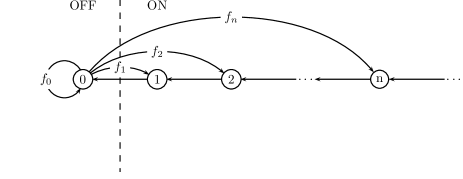
Figure 2: An infinite Markov chain which generates a time series exhibiting LRD.

The chain shown, given a starting state $X_{0}\in\mathbb{Z}_{+}$, produces a Markov time series $\{X_{i}:i\in\mathbb{N}\}$ where all the $X_{i}\in\mathbb{Z}_{+}$. In turn, this chain can generate a time series $\{Y_{i}:i\in\mathbb{N}\}$ where $Y_{i}=0$ if $X_{i}=0$ and $Y_{i}=1$ otherwise.

It can be easily shown that the chain above is ergodic (and hence the equilibrium distribution exists) if $\sum_{i=0}^{\infty}if_{i}<\infty$ and also $\forall i\in\mathbb{N},\exists j>i:f_{j}>0$ — the first condition ensures that the mean return time to the zero state is finite, the second ensures that any state in the chain can be reached from the zero state (obviously the zero state will be reached from any state $i$ in exactly $i$ steps). For the rest of this paper it will be assumed that any chain discussed meets these conditions for ergodicity.

Theorem 1.

The equilibrium distribution of the $i$th state is given by,

$$\pi_{i}=\pi_{0}\sum_{j=i}^{\infty}f_{j}.$$

Proof.

For a state $i$ then at equilibrium, the inputs to a state will sum to $\pi_{i}$. That is,

$$\pi_{i}=\pi_{i+1}+\pi_{0}f_{i}.$$ (2)

Substituting the same equation for $\pi_{i+1}$ gives,

$$\pi_{i}=\pi_{0}f_{i}+\pi_{0}f_{i+1}+\pi_{i+2},$$

and repeating this subsitution recursively gives the proof. ∎

Note that since $\sum_{j=0}^{\infty}f_{j}=1$ then for $i=0$ this equation simply says $\pi_{0}=\pi_{0}$. Since all the $\pi_{i}$ must sum to one then, in addition,

$$\pi_{0}=1-\sum_{i=1}^{\infty}\pi_{i}=(1+\sum_{i=1}^{\infty}if_{i})^{-1},$$

which, as has already been discussed, is finite.

II.1 Introducing LRD into the model

LRD with Hurst parameter $H$ can be guaranteed if the ACF $\rho(k)$ meets the condition given by (1). The most obvious way to induce a correlation for a lag $k$ into such a model is to choose the $f_{i}$ in such a way that unbroken sequences of $k$ or more ones occur in the $Y_{n}$ series with the required frequency. Therefore, it would be suspected that the condition,

$$\mathbb{P}\left[Y_{i}=1,Y_{i+1}=1\dots Y_{i+k}=1\right]\sim Ck^{-\alpha},$$

where $\alpha\in(0,1)$ will produce LRD with $H=1-\alpha/2$. To meet this requirement, the following strict condition is introduced for $k>0$,

$$\sum_{i=k}^{\infty}\pi_{i}=Ck^{-\alpha},$$

where $C$ is a constant. Note that there is no guarantee that this is a valid Markov chain — conditions for this will be given later. By setting $k=1$ it is immediate that $C=1-\pi_{0}$. This gives,

$$\sum_{i=k}^{\infty}\pi_{i}=(1-\pi_{0})k^{-\alpha}\qquad k>0.$$

Subtracting the equation for $k+1$ gives,

$$\pi_{k}=(1-\pi_{0})[k^{-\alpha}-(k+1)^{-\alpha}]\qquad k>0.$$

From (2) for $k$ then,

$$\pi_{0}f_{k}=\pi_{k}-\pi_{k+1}\qquad k>0,$$

and therefore for $k>0$,

$$f_{k}=\frac{1-\pi_{0}}{\pi_{0}}\left[k^{-\alpha}-2(k+1)^{-\alpha}+(k+2)^{-\alpha}\right],$$ (3)

and also, since $f_{0}=1-\sum_{i=1}^{\infty}f_{i}$,

$$f_{0}=1-\frac{1-\pi_{0}}{\pi_{0}}\left[\sum_{i=1}^{\infty}i^{-\alpha}-2\sum_{i=2}^{\infty}i^{-\alpha}+\sum_{i=3}^{\infty}i^{-\alpha}\right].$$

Most of the terms of the sum cancel leaving

$$f_{0}=1-\frac{1-\pi_{0}}{\pi_{0}}\left[1-2^{-\alpha}\right].$$ (4)

The two equations, (3) and (4) form the model for LRD. The model is defined by two parameters $\pi_{0}$ and $\alpha$. The $\alpha$ parameter is related to the Hurst parameter as shown. The $\pi_{0}$ parameter is the equilibrium probability of state zero. Hence $1-\pi_{0}$ is the sum of all other equilibrium probabilities and, therefore, the probability that any given $Y_{i}=1$. Therefore, the expectation value of $Y_{i}$ is given by, $\text{E}\left[Y_{i}\right]=1-\pi_{0}$. It remains to be proved that the model does generate LRD with the required Hurst parameter and this is shown in the next section of the paper.

It can be easily shown that this model meets the conditions for ergodicity established earlier. However, it should be noted that this model is not valid for every possible combination of $\pi_{0}$ and $\alpha$. In particular, for values of $\pi_{0}$ near zero then the term $(1-\pi_{0})/\pi_{0}$ becomes large and values of $f_{i}$ from (3) will be negative, a contradiction since the $f_{i}$ are probabilities. The fact that the model is invalid for some combinations of $\pi_{0}$ and $\alpha$ simply means that for practical experiments the model must be confined to the valid region. Rearranging equation (4) shows that for $\alpha,\pi_{0}\in(0,1)$ then $f_{0}\in(0,1)$ if

$$\pi_{0}>\frac{2^{\alpha}-1}{2^{\alpha+1}-1},$$

and this defines a valid region for the model.

III The ACF of the Markov Model

It must now be shown that the model described in the previous section does produce traffic with a given mean and Hurst parameter. To recap, the model relies on a Markov chain of the form shown in Figure 2 and with transition probabilities given by (3) and (4). The parameters of the model are $\pi_{0}$ and $\alpha$. Given some starting $X_{0}\in\mathbb{Z}_{+}$, the Markov chain produces a time series $\{X_{i}:i\in\mathbb{N}\}$ where $X_{i}$ is the state of the chain at the $i$th iteration. This is used to produce another time series $\{Y_{i}:i\in\mathbb{N}\}$ where $Y_{i}=0$ if $X_{i}=0$ and $Y_{i}=1$ otherwise. (The time series $Y_{i}=1$ if $X_{i}=0$ and $Y_{i}=0$ otherwise also produces a series with LRD and mean $\pi_{0}$.) This series has LRD with mean $1-\pi_{0}$ and Hurst parameter $H=1-\alpha/2$. That $\text{E}\left[Y_{i}\right]=1-\pi_{0}$ has already been shown. It remains to show that the series has an ACF which follows the form in (1) and this requires a result due to Feller (1949) and is based on Wang (1989).

III.1 Proof that the Chain Generates LRD

The event $\varepsilon$ occurs whenever $X_{i}=0$. It can easily be seen that the number of samples between successive occurrences of $\varepsilon$ is an independent and identically distributed variable and hence meets the definition in Feller (1949). A “trial” in the terms of Feller (1949) is equivalent to one iteration of the Markov chain in this model.

Definition 2.

If $\varepsilon$ occurs at the zeroth trial then let the number of occurrences of $\varepsilon$ in $n$ trials be $N_{n}$. Let $F(n)$ be the distribution function of the number of trials between one event $\varepsilon$ and the next. (Note that these definitions are those used by Feller (1949)).

If the event $\varepsilon$ has just occurred (at the zeroth trial) then the chain is in state 0. If the chain makes the transition to state $i-1$ then the event $\varepsilon$ will occur in $i$ steps. Therefore, the distribution function is given by

$$F(n)=\sum_{i=1}^{n}f_{i-1}.$$ (5)

The results from Feller (1949) and Wang (1989) both assume that the distribution function $F(n)$ obeys

$$1-F(n)\sim An^{\gamma},$$ (6)

for some positive constant $A$ and some $\gamma$. This will now be shown for the specified infinite chain.

From equation (5),

$$1-F(n)=1-\sum_{i=1}^{n}f_{i-1}=\sum_{i=n+1}^{\infty}f_{i-1}=\sum_{i=n}^{\infty}f_{i}.$$

Substituting $f_{i}$ from (3):

$$1-F(n) =\left(\frac{1-\pi_{0}}{\pi_{0}}\right)$$

$$\quad\sum_{i=n}^{\infty}\left[i^{-\alpha}-2(i+1)^{-\alpha}+(i+2)^{-\alpha}\right]$$

$$=\left(\frac{1-\pi_{0}}{\pi_{0}}\right)\left[n^{-\alpha}-(n+1)^{-\alpha}\right]$$

$$=\left(\frac{1-\pi_{0}}{\pi_{0}}\right)\frac{(n+1)^{\alpha}-n^{\alpha}}{(n+1)^{\alpha}n^{\alpha}}$$

$$=\left(\frac{1-\pi_{0}}{\pi_{0}}\right)\frac{(1+1/n)^{\alpha}-1}{n^{\alpha}(1+1/n)^{\alpha}}.$$

Expanding $(1+1/n)^{\alpha}$ using the binomial theorem gives

$$(1+1/n)^{\alpha}=1+\alpha/n+O(n^{-2}).$$

Substituting this expression top and bottom gives

$$1-F(n) =\left(\frac{1-\pi_{0}}{\pi_{0}}\right)\frac{1+\alpha/n+O(n^{-2})-1}{n^{\alpha}(1+\alpha/n+O(n^{-2}))}$$

$$=\left(\frac{1-\pi_{0}}{\pi_{0}}\right)\frac{n^{-\alpha}(\alpha/n+O(n^{-2}))}{(1+\alpha/n+O(n^{-2}))}$$

$$\sim\left(\frac{1-\pi_{0}}{\pi_{0}}\right)\alpha n^{-(1+\alpha)},$$

where $f(n)=O(g(n))$ for functions $f(n)$ and $g(n)$ means that $|f(n)|<Ag(n)$ for some positive constant $A$ and all $n>0$. This is the form required by equation (6) with $\gamma=(1+\alpha)$ and $A=\alpha(1-\pi_{0})/\pi_{0}$.

From (Feller, 1949, Theorem 10), given that the probability distribution satisifies $1-F(x)\sim Ax^{-\gamma}$, where $A$ is a positive constant and $1<\gamma<2$ then

$$\text{var}\left(N_{n}\right)\sim\frac{2A}{(2-\gamma)(3-\gamma)\mu^{3}}n^{3-\gamma}.$$

In the case of the chain under investigation $\gamma=1+\alpha$, and $A=\alpha(1-\pi_{0})/\pi_{0}$. Since the chain is ergodic, the mean recurrence time of state zero for the infinite chain is $1/\pi_{0}$. Therefore,

$$\text{var}\left(N_{n}\right)\sim\frac{2\alpha\pi_{0}^{2}(1-\pi_{0})}{(1-\alpha)(2-\alpha)}n^{2-\alpha}.$$ (7)

From Wang (1989) (equations 2.26a and 2.26c) if

$$\text{var}\left(N_{n}\right)\sim Kn^{2-\alpha},$$

for some positive constant $K$ and some $\alpha\in(0,1)$ then the autocorrelation function is given by

$$\rho(n)\sim Cn^{-\alpha},$$

where $C$ is some positive constant. This is the form required by (1).

IV Tests on the Markov Model

In this section, two standard models for generating LRD are compared with the Markov model described in this paper. The computational performance of the algorithm is compared against other algorithms.

IV.1 Practical Implementation of the Model

The only difficulty in modelling the situation on a computer comes in calculating $X_{n+1}$ when $X_{n}=0$. In this case, a random number generator and the transition probabilities $f_{j}$ must be used to find the next state. A naive approach to this would be to generate a random number $r$, uniformly distributed in $(0,1)$ and say that $X_{n+1}$ is the smallest $i$ such that $\sum_{j=0}^{i}f_{i}<r$. This is fine for low values of $i$ but as $i$ increases then this procedure becomes inaccurate due to the finite precision arthmetic used by computers. The problem is that, as $i$ increases the sum gets nearer to one but the $f_{i}$ get nearer to zero (since adding numbers approaching zero to numbers approaching one is likely to produce severe rounding error problems). Hence the errors in each stage of addition get larger. However, by the very nature of LRD, large values of $i$ are very likely to come up.

It can simply be shown that if $X_{n}=0$ and $0<k\leq i\leq j$,

$$\begin{split}\mathbb{P}\left[X_{n+1}\in[i,j]|X_{n+1}\in[k,\infty]\right]=\\ \frac{i^{-\alpha}-(i+1)^{-\alpha}-(j+1)^{-\alpha}+(j+2)^{-\alpha}}{k^{-\alpha}-(k+1)^{-\alpha}}.\end{split}$$ (8)

Using this equation, Table 1 shows a procedure for generating the sequence $\{X_{n}:n\in\mathbb{N}\}$ given some randomly chosen $X_{0}$.

 

1. If $X_{n}>0$ then $X_{n+1}=X_{n}-1$. Exit here.

2. Explicitly calculate $\mathbb{P}\left[X_{n+1}>j\right]$ for values of $j\leq N$ where $N$ is some small integer. Use the procedure for the finite state model to find a value for $X_{n+1}$ if $X_{n+1}<N$.

3. Generate a new random number $R$ in the range $[0,1]$.

4. Calculate $\mathbb{P}\left[X_{n+1}\in[N,2N-1]|X_{n+1}\in[N,\infty]\right]$ from equation (8). If $R$ is less than or equal to this probability then $X_{n+1}$ is in the required range. Otherwise go to step six.

5. If $X_{n+1}$ is in the required range then refine down by generating a new random number and seeing if $X_{n+1}$ is in the range $[N,(3/2)N]$. Continue refining by a binary search (with a new random number each time) until $X_{n+1}$ is found. Exit here.

6. Increase the value of $N$ to $2N$ and go to step 3.

 

Table 1: A procedure for finding $X_{n+1}$ from $X_{n}$ in the infinite chain.

IV.2 Hurst Parameter Estimates

Three generation mechanisms for LRD are compared, Fractional Gaussian Noise (FGN), iterated maps (it. map) and the Markov method developed in this paper. For each method, three different Hurst parameters are investigated and for each of these, three data realisations are created. For each realisation, one million points were generated (in the case of the iterated map and Markov method, each of those points was an aggregate of one hundred zeros and ones). The Hurst parameter was estimated using the previously discussed measurement techniques to check the match between theory and experiment.

The three methods were implemented in the C programming language. On a 2GHz processor PC running Debian linux, to generate one million points took 55 seconds for the Markov method, 60 seconds for the iterated maps method and 6 seconds for the fractional Gaussian noise method. However, it is debatable whether this is a fair comparison since the first two methods could be considered to be generating a hundred million points and aggregating into groups of one hundred. No C code to generate FARIMA based data was available and the R code available took 188 seconds to generate only a hundred thousand points — the run time did not seem to scale linearly and the test to generate a million points was stopped after several hours.

Source	H	R/S	Mod.	Agg.	Period-	Local	Wave-
			R/S	Var.	ogram	Whit.	lets
FGN	0.625	0.637	0.624	0.623	0.626	0.639	0.635
FGN	0.625	0.632	0.624	0.622	0.624	0.638	0.635
FGN	0.625	0.645	0.633	0.620	0.622	0.638	0.635
FGN	0.75	0.728	0.738	0.741	0.747	0.774	0.767
FGN	0.75	0.741	0.736	0.749	0.755	0.776	0.769
FGN	0.75	0.694	0.719	0.741	0.754	0.774	0.768
FGN	0.875	0.784	0.837	0.858	0.877	0.908	0.897
FGN	0.875	0.750	0.823	0.850	0.876	0.908	0.897
FGN	0.875	0.747	0.835	0.860	0.876	0.908	0.898
It. map	0.625	0.635	0.590	0.604	0.630	0.719	0.706
It. map	0.625	0.608	0.595	0.604	0.627	0.716	0.703
It. map	0.625	0.637	0.594	0.610	0.637	0.718	0.707
It. map	0.75	0.828	0.666	0.717	0.746	0.813	0.800
It. map	0.75	0.725	0.650	0.712	0.739	0.813	0.801
It. map	0.75	0.678	0.694	0.765	0.768	0.814	0.803
It. map	0.875	0.703	0.779	0.851	0.876	0.925	0.910
It. map	0.875	0.779	0.802	0.854	0.877	0.924	0.910
It. map	0.875	0.846	0.817	0.861	0.874	0.925	0.912
Markov	0.625	0.526	0.597	0.611	0.621	0.703	0.691
Markov	0.625	0.593	0.645	0.700	0.684	0.710	0.702
Markov	0.625	0.632	0.603	0.646	0.650	0.707	0.698
Markov	0.75	0.663	0.684	0.744	0.760	0.793	0.784
Markov	0.75	0.670	0.667	0.751	0.759	0.793	0.783
Markov	0.75	0.671	0.671	0.724	0.736	0.786	0.776
Markov	0.875	0.724	0.732	0.816	0.848	0.884	0.873
Markov	0.875	0.757	0.754	0.830	0.859	0.885	0.874
Markov	0.875	0.656	0.781	0.852	0.866	0.885	0.875

Table 2: Hurst Parameter Estimates on Simulated Data.

It would naturally be expected that the FGN model is the easiest to estimate and this shows in the results in Table 2. All the estimators were relatively close to correct with the possible exception of the R/S plot on traffic with a Hurst parameter of 0.875 where the underestimate of $H$ was quite severe.

Estimates on the iterated chaotic map traffic were not so successful. The raw R/S plot proved inconsistent and had a hard time estimating higher hurst parameters. It should be noted, for example, that for $H=0.75$ estimates varied from 0.678 to 0.828. The performance for $H=0.875$ was similarly bad. The modified R/S parameter was better in that it was more stable across runs but tended to overestimate. Local Whittle and wavelets tended to overestimate the Hurst parameter. It should also be noted that the true result was regularly outside the 95% confidence intervals for the wavelet estimator.

Estimates for the Markov based method were, in many ways, similar to the iterated map method. If anything, the results from the estimators are slightly closer to the theory and this is particularly notable for the wavelet and local Whittle case. The evidence provided by the estimators is hard to interpret. However, it can certainly be said that the results for the Markov method are as close as the results for the iterated map method.

Generally, considering the estimators themselves, the R/S method seemed unreliable (and this agrees with theory which shows it to be a biased estimator with poor convergence). The local Whittle and wavelets methods which have better theoretical backing seem to have a better agreement with theory but it is worrying that the true Hurst parameter for the data lay outside 95% confidence for the wavelet estimator in many cases.

V Conclusions

The method for generating LRD shown here is computationally efficient, extremely simple and produces a data stream with a given mean and Hurst paramter. The data stream can be generated in an online manner (that is, the method can be started without knowing how many points must ultimately be generated unlike, for example, FGN). The method has been proved theoretically to generate LRD with the required parameters and this has been tested against a variety of known estimators for the Hurst parameter. It is interesting to see quite how badly certain estimators perform even against very standard LRD generation mechanisms.

Compared with existing methods of generating LRD this procedure has a number of extremely attractive properties. It is computationally and mathematically extremely simple. While other models may have more flexibility for precisely representing the nature of the time series being simulated, it is hard to imagine a simpler model for generating LRD. It is hoped, therefore, that this model will be tractable analytically for further developments, for example, analysis of queuing performance of traffic generated by such a model.