Theory and Practice of Triangle Problems
in Very Large (Sparse (Power-Law)) Graphs

Abstract

Finding, counting and/or listing triangles (three vertices with three edges) in large graphs are natural fundamental problems, which received recently much attention because of their importance in complex network analysis. We provide here a detailed state of the art on these problems, in a unified way. We note that, until now, authors paid surprisingly little attention to space complexity, despite its both fundamental and practical interest. We give the space complexities of known algorithms and discuss their implications. Then we propose improvements of a known algorithm, as well as a new algorithm, which are time optimal for triangle listing and beats previous algorithms concerning space complexity. They have the additional advantage of performing better on power-law graphs, which we also study. We finally show with an experimental study that these two algorithms perform very well in practice, allowing to handle cases that were previously out of reach.

1 Introduction.

A triangle in an undirected graph is a set of three vertices such that each possible edge between them is present in the graph. Following classical conventions, we call finding, counting and listing the problems of deciding if a given graph contains any triangle, counting the number of triangles in the graph, and listing all of them, respectively. We moreover call pseudo-listing the problem of counting for each vertex the number of triangles to which it belongs. We refer to all these problems as a whole by triangle problems.

Triangle problems may be considered as classical, natural and fundamental algorithmic questions, and have been studied as such [23, 14, 2, 3, 32, 33].

Moreover, they gained recently much practical importance since they are central in so-called complex network analysis, see for instance [35, 13, 1, 19]. First, they are involved in the computation of one of the main statistical property used to describe large graphs met in practice, namely the clustering coefficient [35]. The clustering coefficient of a vertex $v$ (of degree at least $2$) is the probability that any two randomly chosen neighbors of $v$ are linked together. It is computed by dividing the number of triangles containing $v$ by the number of possible edges between its neighbors, i.e. $d(v)\choose 2$ if $d(v)$ denotes the number of neighbors of $v$. One may then define the clustering coefficient of the whole graph as the average of this value for all the vertices (of degree at least $2$). Likewise, the transitivity ratio  [21, 20] is defined as $\frac{3\cdot N_{\Delta}}{N_{\vee}}$ where $N_{\Delta}$ denotes the number of triangles in the graph and $N_{\vee}$ denotes the number of connected triples, i.e. sets of three vertices with at least two edges, in the graph.

In the context of complex network analysis, triangles also play a key role in the study of motif occurrences, i.e. the presence of special (small) subgraphs in given (large) graphs. This has been studied in particular in protein interaction networks, where some motifs may correspond to biological functions, see for instance [28, 36]. Triangles often are building blocks of these motifs.

Finally, triangle finding, counting, pseudo-listing and/or listing appear as key issues both from a fundamental point of view and for practical purpose. The aim of this contribution is to review the algorithms proposed until now for solving these problems with both a fundamental perspective (we discuss asymptotic complexities and give detailed proofs) and a practical one (we discuss space requirements and graph encoding, and we evaluate algorithms with some experiments).

We note that, until now, authors paid surprisingly little attention to space requirements of their algorithms for triangle problems; this however is an important limitation in practice, and this also induces interesting theoretical questions. We will therefore discuss this (all space complexity results stated in this paper are new, though very simple in most cases), and we will propose space-efficient algorithms.

The paper is organised as follows. After a few preliminaries (Section 2), we begin with results on finding, counting and pseudo-listing problems, between which basically no difference in complexity is known (Section 3). Then we turn to the harder problem of triangle listing, in Section 4. In these parts of the paper, we deal with both the general case (no assumption is made on the graph) and on the important case where the graph is sparse. Many very large graphs met in practice also have heterogeneous degrees; we focus on this case in Section 5. Finally, we present experimental evaluations in Section 6. We summarise the current state of the art and we point out the main perspectives in Section 7.

2 Preliminaries.

Throughout the paper, we consider an undirected  graph $G=(V,E)$ with $n=|V|$ vertices and $m=|E|$ edges. We suppose that $G$ is simple ($(v,v)\not\in E$ for all $v$, and there is no multiple edge). We also assume that $m\in\Omega(n)$; this is a classical convention which plays no role in our algorithms but makes complexity formulae simpler. We denote by $N(v)\ =\ \{u\in V,\ (v,u)\in E\}$ the neighborhood of $v\in V$ and by $d(v)=|N(v)|$ its degree. We also denote by $d_{\max}$ the maximal degree in $G$: $d_{\max}=\max_{v}\{d(v)\}$.

Before entering in the core of this paper, we need to discuss a few issues that will play an important role in the following. They are necessary to make the discussion all along the paper precise and rigorous.

Graph encodings.

First note that we will always suppose that the graph is stored in central memory . There are basically two ways to do this:

• $G$ may be encoded by its adjacency matrix $A$ defined by $A_{ij}=1$ if $(i,j)\in E$, $A_{ij}=0$ else. This has a $\Theta(n^{2})$ space cost. Since $m$ may be up to $\Theta(n^{2})$, this representation is space optimal in this case (but it is not as soon as the graph is sparse, i.e. $m\in o(n^{2})$), and makes it possible to test the presence of any edge in $\Theta(1)$. Note however that one cannot run through $N(v)$ in $O(d(v))$ time with such a representation: one needs $\Theta(n)$ time. Since $d(v)$ may be up to $\Theta(n)$, this is not a problem in the general case.

• $G$ may be encoded by a simple compact representation: for each vertex $v$ we can access the set of its neighbors $N(v)$ and its degree $d(v)$ in $\Theta(1)$ time and space cost. The set $N(v)$ usually is encoded using a linked list or an array, in order to be able to run through it in $\Theta(d(v))$ time and $\Theta(1)$ space. It may moreover be sorted (an order on the vertices is supposed to be given). This representation has the advantage of being space efficient: it needs only $\Theta(m)$ space. However, testing the presence of the edge $(u,v)$ is in $\Theta(d(v))$ time ($O(\log(d(v)))$ if $N(v)$ is a sorted array). We call any representation having these properties a simple compact representation of $G$.

Since the basic operations of such representations do not have the same complexity, they may play a key role in algorithms using them. We will see that this is indeed the case in our context. We note moreover that, in the context of large graph manipulation, the adjacency matrix often is untractable because of its space requirements. This is why one generally uses (sorted) simple compact representations in practice.

One may easily convert any simple compact representation of $G$ into its adjacency array representation, in time $\Theta(m)$ using $\Theta(n)$ additional space (it suffices to transform iteratively each set $N(v)$ and to free the memory used by the previous representation at each step). Moreover, once the adjacency array representation of $G$ is available, one may compute its sorted version in $\Theta\left(\sum_{v}d(v)\cdot\log(d(v))\right)\ \subseteq\ O\left(\sum_{v}d(v)\cdot\log(n)\right)\ =\ O(m\cdot\log(n))$ time and $\Theta(1)$ additional space. One may therefore intuitively make no difference between any simple compact representation of $G$ and its sorted adjacency array representation, as long as the overall algorithm complexity is in $\Omega(m\cdot\log(n))$ time and $\Omega(n)$ space.

One may also obtain a simple compact representation of $G$ from its adjacency matrix in time $\Theta(n^{2})$ and additional space $\Theta(n)$ (provided that one does not need the matrix anymore, else it costs $\Theta(m)$). This cost is not neglectible in most cases, and thus we will suppose that algorithms that need the two representations receive them both as inputs.

Finally, note that one may use more subtle structures to encode the sets $N(v)$ for all $v$. Balanced trees and hashtables are the most classical ones. Since we focus on worst case analysis (see below), such encodings have no impact on our results, and so we make no difference between them and any other simple compact representation.

(Additional) Space complexity.

As explained above, storing the graph itself generally is in $\Theta(n^{2})$ or $\Theta(m)$ space complexity. Moreover, the space requirements of the algorithms we will study are, in most cases, lower than the space requirements of the graph storing. Therefore, their space complexity is the one of the chosen graph representation, which makes little sense.

However, limiting the space needed by the algorithm in addition to the one needed to store the graph often is a key issue in practice: current main limitation in triangle problems on real-world complex networks is space requirements. We illustrate this in Section 6.

For these reasons, the space complexities we discuss concern the additional space needed by the algorithm, i.e. not including the graph storage. As we will see, this notion makes a significant difference between various algorithms, and therefore also has a fundamental interest.

Likewise, and following classical conventions, we do not include the size of the output in our space complexities. Otherwise, triangle listing would need $\Omega(n^{3})$ space in the worst case, and pseudo-listing would need $\Omega(n)$ space, which brings little information, if any.

Worst case complexity, and graph families.

All the complexities we discuss in this paper are worst case complexities, in the sense that they are bounds for the time and space needs of the algorithms, on any input. In most cases, these bounds are tight (leading to the use of the $\Theta()$ notation, see for instance [17] for definitions). In other words, we say that an algorithm is in $\Theta(f(n))$ if there exists an instance of the input such that the algorithm runs with this complexity (even if some instances induce lower complexity). In several case, however, the worst case complexity actually is the complexity for any input (in the case of Theorem 4, for instance, and for most space complexities).

It would also be of high interest to study the expected behavior of triangle algorithms, in addition to the worst case one. This has been done in some cases; for instance, it is proved in [23] that vertex-iterator (see Section 4.1) has expected time complexity in $O(n^{\frac{5}{3}})$. Obtaining such results however often is very difficult, and their relevance for practical purpose is not always clear: the choice of a model for the average input is a difficult task (in our context, random graphs would be an unsatisfactory choice [13, 1, 35]). We therefore focus on worst case analysis, which has the advantage of giving guarantees on the behaviors of algorithms, on any input.

Another interesting approach is to study (worst case) complexities on given graph families. This has already been done on various cases, the most important ones probably being the sparse graphs, i.e. graphs in which $m$ is in $o(n^{2})$. This is motivated by the fact that most real-world complex networks lead to such graphs, see for instance [13, 1, 35]. In general, it is even assumed that $m$ is in $O(n)$. Recent studies however show that, despite the fact that $m$ is small compared to $n^{2}$, it may be in $\omega(n)$ [27, 30, 26]. Other classes of graphs have been considered, like for instance planar graphs: it is shown in [23] that one may decide if any planar graph contains a triangle in $O(n)$ time.

We do not detail all these results here. Since we are particularily interested in real-world complex networks, we present in detail the results concerning sparse graphs all along the paper. We also introduce new results on power-law graphs (Section 5), which capture an important property met in practice. A survey on available results on specific classes of graphs remains to be done, and is out of the scope of this paper.

3 The fastest algorithms for finding, counting, and pseudo-listing.

The fastest algorithm known for pseudo-listing relies on fast matrix product [23, 2, 3, 16]. Indeed, if one considers the adjacency matrix $A$ of $G$ then the value $A^{3}_{vv}$ on the diagonal of $A^{3}$ is nothing but twice the number of triangles to which $v$ belongs, for any $v$. Finding, counting and pseudo-listing triangle problems can therefore be solved in $O(n^{\omega})$ time, where $\omega<2.376$ is the fast matrix product exponent [16]. This was first noticed in 1978 [23], and currently no faster algorithm is known for any of these problems in the general case, even for triangle finding (but this is no longer true when the graph is sparse, see Theorem 2 below).

This approach naturally needs the graph to be given by its adjacency matrix representation. Moreover, it makes it necessary to compute and store the matrix $A^{2}$, leading to a $\Theta(n^{2})$ space complexity in addition to the adjacency matrix storage.

Theorem 1 ([23, 16])

Given the adjacency matrix representation of $G$, it is possible to solve triangle finding, counting and pseudo-listing in $O(n^{\omega})\subset O(n^{2.376})$ time and $\Theta(n^{2})$ space on $G$ using fast matrix product.

This time complexity is the current state of our knowledge, as long as one makes no assumption on $G$. Note that no lower bound is known for this complexity; therefore faster algorithms may be designed.

As we will see, there exists (slower) algorithms with lower space complexity for these problems. Some of these algorithms only need a simple compact representation of $G$. They are derived from listing algorithms, which we present in Section 4.

One can design faster algorithms if $G$ is sparse. In [23], it was first proved that triangle finding, counting, pseudo-listing and listing  can be solved in $\Theta(m^{\frac{3}{2}})$ time and $\Theta(m)$ space. This result has been improved in [14] using a property of the graph (namely arboricity) but the worst case complexites were unchanged. No better result was known until 1995 [3, 2], where the authors prove Theorem 2 below , which constitutes a significant improvement although it relies on very simple ideas. We detail the proof and give a slightly different version, which will be useful in the following (similar ideas are used in Section 4.3, and this proof permits a straightforward extension of this theorem in Section 5).

Input: any simple compact representation of $G$, its adjacency matrix $A$, and an integer $K$
Output: $T$ such that $T[v]$ is the number of triangles in $G$ containing $v$
1. initialise $T[v]$ to $0$ for all $v$
2. for each vertex $v$ with $d(v)\leq K$:
  2a. for each pair $\{u,w\}$ of neighbors of $v$:
    2aa. if $A[u,w]$ then:
      2aaa. increment $T[v]$
      2aab. if $d(u)>K$ and $d(w)>K$ then increment $T[u]$ and $T[w]$
      2aac. else if $d(u)>K$ and $u>v$ then increment $T[u]$
      2aad. else if $d(w)>K$ and $w>v$ then increment $T[w]$
3. let $G^{\prime}$ be the subgraph of $G$ induced by $\{v,\ d(v)>K\}$
4. construct the adjacency matrix $A^{\prime}$ of $G^{\prime}$
5. compute $A^{\prime 3}$ using fast matrix product
6. for each vertex $v$ with $d(v)>K$:
  6a. add to $T[v]$ half the value in $A^{\prime 3}_{vv}$

Algorithm 1 – ayz-pseudo-listing. Counts for all $v$ the triangles in $G$ containing $v$ [3, 2].

Theorem 2 ([3, 2])

Given any simple compact representation of $G$ and its adjacency matrix, it is possible to solve triangle finding, counting and pseudo-listing on $G$ in $O(m^{\frac{2\cdot\omega}{\omega+1}})\subset O(m^{1.41})$ time and $\Theta\left(m^{\frac{4}{\omega+1}}\right)\subset O(m^{1.185})$ space; Algorithm 1 (ayz-pseudo-listing) achieves this if one takes $K\in\Theta(m^{\frac{\omega-1}{\omega+1}})$.

Proof: Let us first show that Algorithm 1 (ayz-pseudo-listing) solves pseudo-listing (and thus counting and finding). Consider a triangle in $G$ that contains a vertex with degree at most $K$; then it is discovered in lines 2a and 2aa. Lines 2aaa to 2aad ensure that it is counted exactly once for each vertex it countains. Consider now the triangles in which all the vertices have degree larger than $K$. Each of them induces a triangle in $G^{\prime}$, and $G^{\prime}$ contains no other triangle. These triangles are counted using the matrix product approach (lines 5, 6 and 6a), and finally all the triangles in $G$ are counted for each vertex.

Let us now study the time complexity of Algorithm 1 (ayz-pseudo-listing) in function of $K$. For each vertex $v$ with $d(v)\leq K$, one counts the number of triangles containing $v$ in $\Theta(d(v)^{2})\subseteq O(d(v)\cdot K)$ thanks to the simple compact representation of $G$. If we sum over all the vertices in the graph this leads to a time complexity in $O(m.K)$ for lines 2 to 2aad. Now notice that there cannot be more than $\frac{2\cdot m}{K}$ vertices $v$ with $d(v)>K$. Line 4 constructs (in $O\left(m+(\frac{m}{K})^{2}\right)$ time, which plays no role in the global complexity) the adjacency matrix of the subgraph $G^{\prime}$ of $G$ induced by these vertices. Using fast matrix product, line 5 computes the number of triangles for each vertex in $G^{\prime}$ in time $O\left(\left(\frac{m}{K}\right)^{\omega}\right)$. Finally, we obtain the overall time complexity of the algorithm: $O\left(m.K+\left(\frac{m}{K}\right)^{\omega}\right)$.

In order to minimize this, one has to search for a value of $K$ such that $m\cdot K\in\Theta((\frac{m}{K})^{\omega})$. This leads to $K\in\Theta(m^{\frac{\omega-1}{\omega+1}})$, which gives the announced time complexity.

Concerning space complexity, the key point is that one has to construct $A^{\prime}$, $A^{\prime 2}$ and $A^{\prime 3}$. The matrix $A^{\prime}$ may contain $\frac{2\cdot m}{K}$ vertices, leading to a $\Theta\left(\left(\frac{m}{K}\right)^{2}\right)=\Theta\left(m^{2\cdot\left(1-\frac{\omega-1}{\omega+1}\right)}\right)=\Theta\left(m^{\frac{4}{\omega+1}}\right)$ space complexity. $\Box$

Note that one may also use sparse matrix product algorithms, see for instance [38]. However, the matrix $A^{2}$ may not be sparse (in particular if there are vertices with large degrees, which is often the case in practice as discussed in Section 5). But algorithms may take benefit from the fact that one of the two matrices involved in a product is sparse, and there also exists algorithms for products of more than two sparse matrices. These approaches lead to algorithms whose efficiency depends on the exact relation between $m$ and $n$: it depends on the relation between $n$ and $m$ which algorithm is the fastest. Discussing this further therefore is quite complex, and it is out of the scope of this paper.

In conclusion, despite the fact that the algorithms presented in this section are asymptotically very fast, they have two important limitations. First, they have a prohibitive space cost, since the matrices involved in the computation (in addition to the adjacency matrix, but it is considered as the encoding of $G$ itself) may need $\Theta(n^{2})$ space. Moreover, the fast matrix product algorithms are quite intricate, which leads to difficult implementations with high risks of errors. This also leads to large constant factors in the complexities, which have no importance at the asymptotic limit but may play a significant role in practice.

For these reasons, and despite the fact that they clearly are of prime theoretical importance, these algorithms have limited practical impact. Instead, one generally uses one of the listing algorithms (adapted accordingly) that we detail now.

4 Time-optimal listing algorithms.

First notice that there may be ${n\choose 3}\in\Theta(n^{3})$ triangles in $G$. Likewise, there may be $\Theta(m^{\frac{3}{2}})$ triangles, since $G$ may be a clique of $\sqrt{m}$ vertices (thus containing ${\sqrt{m}\choose 3}\in\Theta(m^{\frac{3}{2}})$ triangles). This gives the following lower bounds for the time complexity of any triangle listing algorithm.

Lemma 3 ([23, 32, 33])

Listing all triangles in $G$ is in $\Omega(n^{3})$ and $\Omega(m^{\frac{3}{2}})$ time.

In this section, we first observe that the time complexity $\Theta(n^{3})$ can easily be reached (Section 4.1). However, $\Theta(m^{\frac{3}{2}})$ is much better in the case of sparse graphs. We present more subtle algorithms that reach this bound (Section 4.2). Again, space complexity is a key issue, and we discuss this for each algorithm. We will see that algorithms proposed until now either rely on the use of adjacency matrices and/or have a $\Omega(m)$ space complexity. We improve this by proposing algorithms that reach a $\Theta(n)$ space complexity, while needing only a simple compact representation of $G$, and still in $\Theta(m^{\frac{3}{2}})$ time (Section 4.3).

4.1 Basic algorithms.

One may trivially obtain a listing algorithm in $\Theta(n^{3})$ (optimal) time with the matrix representation of $G$ by testing in $\Theta(1)$ time any possible triple of vertices. Moreover, this algorithm has the optimal space complexity $\Theta(1)$.

Theorem 4 ([32, 33] and folklore)

Given the adjacency matrix representation of $G$, it is possible to solve triangle listing in $\Theta(n^{3})$ time and $\Theta(1)$ space using the direct testing of every triple of vertices.

This approach however has severe drawbacks. First, it needs the adjacency matrix of $G$. More importantly, its complexity does not depend on the actual properties of $G$; it always needs $\Theta(n^{3})$ computation steps even if the graph contains very few edges. It must however be clear that, if almost all triples of vertices form a triangle, no better asymptotic bound can be attained, and the simplicity of this algorithm makes it very efficient in these cases.

In order to obtain faster algorithms on sparse graphs, while keeping the implementation very simple, one often uses the following algorithms. The first one, introduced in [23] and called vertex-iterator in [32, 33], consists in iterating Algorithm 2 (vertex-listing) on each vertex of $G$. The second one, which seems to be the most widely used algorithm , consists in iterating Algorithm 3 (edge-listing) over each edge in $G$. It was also first introduced in [23], and discussed in [32, 33] where the authors call it edge-iterator.

Input: any simple compact representation of $G$, its adjacency matrix $A$, and a vertex $v$
Output: all the triangles to which $v$ belongs
1. for each pair $\{u,w\}$ of neighbors of $v$:
  1a. if $A_{uw}=1$ then output triangle $\{u,v,w\}$

Algorithm 2 – vertex-listing. Lists all the triangles containing a given vertex [23].

Input: any sorted simple compact representation of $G$, and an edge $(u,v)$ of $G$
Output: all the triangles in $G$ containing $(u,v)$
1. for each $w$ in $N(u)\cap N(v)$:
  1a. output triangle $\{u,v,w\}$

Algorithm 3 – edge-listing. Lists all the triangles containing a given edge [23].

Theorem 5 ([23, 32, 33])

Given any simple compact representation of $G$ and its adjacency matrix, it is possible to list all its triangles in $\Theta\left(\sum_{v}d(v)^{2}\right)$, $\Theta(m\cdot d_{\max})$, $\Theta(m\cdot n)$, and $\Theta(n^{3})$ time and $\Theta(1)$ space; vertex-iterator achieves this.

Proof: The fact that Algorithm 2 (vertex-listing) list all the triangles to which a vertex $v$ belongs is straightforward. Then, iterating over all vertices gives three times each triangle; if one wants each triangle only once it is sufficient to restrict the output of triangles to the ones for which $\eta(w)>\eta(v)>\eta(u)$, for any injective numbering $\eta()$ of the vertices.

Thanks to the simple compact representation of $G$, the pairs of neighbors of $v$ may be computed in $\Theta(d(v)^{2})$ time and $\Theta(1)$ space (this would be impossible with the adjacency matrix only). Thanks to the adjacency matrix, the test in line 1a may be processed in $\Theta(1)$ time and space (this would be impossible with the simple compact representaton only). The time complexity of Algorithm 2 (vertex-listing) therefore is in $\Theta(d(v)^{2})$ time and $\Theta(1)$ space. The $\Theta(\sum_{v}d(v)^{2})$ time and $\Theta(1)$ space complexity of the overall algorithm follows. Moreover, we have $\Theta(\sum_{v}d(v)^{2})\subseteq O(\sum_{v}d(v)\cdot d_{\max})=O(m\cdot d_{\max})\subseteq O(m\cdot n)\subseteq O(n^{3})$, and all these complexity may be attained in the worst case (clique of $n$ vertices), hence the results. $\Box$

Theorem 6 ([23, 32, 33] and folklore)

Given any sorted simple compact representation of $G$, it is possible to list all its triangles in $\Theta(m\cdot d_{\max})$, $\Theta(m\cdot n)$ and $\Theta(n^{3})$ time and $\Theta(1)$ space; The edge-iterator algorithm achieves this.

Proof: The correctness of the algorithm is immediate. One may proceed like in the proof of Theorem 5 to obtain each triangle only once.

Each edge $(u,v)$ is treated in time $\Theta(d(u)+d(v))$ (because $N(u)$ and $N(v)$ are sorted) and $\Theta(1)$ space. We have $d(u)+d(v)\in\Theta(d_{\max})$, therefore the overall complexity is in $O(m\cdot d_{\max})\subseteq O(m\cdot n)\subseteq O(n^{3})$. In the worst case (clique of $n$ vertices) all these complexity are tight. $\Box$

First note  that these algorithms are optimal in the worst case, just like the direct method (Lemma 3 and Theorem 4). However, there are much more efficient on sparse graphs, in particular if the maximal degree is low [7], since they both are in $\Theta(m\cdot d_{\max})$ time. If the maximal degree is a constant, vertex-iterator even is in $\Theta(n)$ time. Moreover, both algorithms only need $\Theta(1)$ space, which makes them very interesting from this perspective (we will see that there is no known faster algorithm with this space requirement).

However, vertex-iterator has a severe drawback: it needs the adjacency matrix of $G$ and a simple compact representation. Instead, edge-iterator only needs a sorted simple compact representation, which is often available in practice . Moreover, edge-iterator runs in $\Theta(1)$ space, which makes it very compact. Because of these two reasons, and because of its simplicity, it is widely used in practice.

The performance of these algorithms however are quite poor when the maximal degree is unbounded, and in particular if it grows like $n$. They may even be asymptotically sub-optimal on sparse graphs and/or on graphs with some vertices of high degree, which often appear in practice (we discuss this further in Section 5). It is however possible to design time-optimal listing algorithms for sparse graphs, which we detail now.

4.2 Time-optimal listing algorithms for sparse graphs.

Several algorithms have been proposed that reach the $\Theta(m^{\frac{3}{2}})$ bound of Lemma 3, and thus are time optimal on sparse graphs (note that this is also optimal for dense graphs, but we have seen in Section 4.1 much simpler algorithms for these cases). Back in 1978, an algorithm was proposed to find a triangle in $\Theta(m^{\frac{3}{2}})$ time and $\Theta(m)$ space [23]. Therefore it is slower than the ones discussed in Section 3 for finding, but it may be extended to obtain a listing algorithm with the same complexity. We first present this below. Then, we detail two simpler solutions with this complexity, proposed recently in [32, 33]. The first one consists in a simple extension of Algorithm 1 (ayz-pseudo-listing); the other one, named forward, has the advantage of being very efficient in practice [32, 33]. Moreoever, we show in Section 4.3 that it may be slightly modified to reach a $\Theta(n)$ space cost.

An approach based on covering trees [23].

We use here the classical notions of covering trees and connected components, as defined for instance in [17]. Since they are very classical, we do not recall them. We just note that a covering tree of each connected component of any graph may be computed in time linear in the number of edges of this graph, and space linear in its number of vertices (typically using a breadth-first search). One then has access to the father of any vertex in $\Theta(1)$ time and space.

In [23], the authors propose a triangle finding algorithm in $\Theta(m^{\frac{3}{2}})$ time and $\Theta(m)$ space. We present here a simple extension of this algorithm to solve triangle listing with the same complexity. To achieve this, we need the following lemma, which is a simple extension of Lemma 4 in [23].

Lemma 7 ([23])

Let us consider a covering tree for each connected component of $G$, and a triangle $t$ in $G$ having an edge in one of these trees. Then there exists an edge $(u,v)$ in $E$ but in none of these trees, such that $t=\{u,v,\mbox{father}(v)\}$.

Proof: Let $t=\{x,y,z\}$ be a triangle in $G$, and let $T$ be the tree that contains an edge of $t$. We can suppose without loss of generality that this edge is $(x,y=\mbox{father}(x))$. Two cases have to be considered. First, if $(x,z)\not\in T$ then it is in none of the trees, and taking $v=x$ and $u=z$ satisfies the claim. Second, if $(x,z)\in T$ then we have $\mbox{father}(z)=x$ (because $\mbox{father}(x)=y\not=z$). Moreover, $(y,z)\not\in T$ (else $T$ would contain a cycle, namely $t$). Therefore taking $v=z$ and $u=y$ satisfies the claim. $\Box$

Input: any simple compact representation of $G$, and its adjacency matrix $A$
Output: all the triangles in $G$
1. while there remains an edge in $E$:
  1a. compute a covering tree for each connected component of $G$
  1b. for each edge $(u,v)$ in none of these trees:
    1ba. if $(\mbox{father}(u),v)\in E$ then output triangle $\{u,v,\mbox{father}(u)\}$
    1bb. else if $(\mbox{father}(v),u)\in E$ then output triangle $\{u,v,\mbox{father}(v)\}$
  1c. remove from $E$ all the edges in these trees

Algorithm 4 – tree-listing. Lists all the triangles in a graph [23].

This lemma shows that, given a covering tree of each connected component of $G$, one may find triangles by checking for each edge $(u,v)$ that belongs to none of these trees if $\{u,v,\mbox{father}(v)\}$ is a triangle. Then, all the triangles containing $(v,\mbox{father}(v))$ are discovered. This leads to Algorithm 4 (tree-listing), and to the following result (which is a direct extension of the one concerning triangle finding described in [23]).

Theorem 8 ([23])

Given any simple compact representation of $G$ and its adjacency matrix, it is possible to list all its triangles in $\Theta(m^{\frac{3}{2}})$ time and $\Theta(n)$ space; Algorithm 4 (tree-listing) achieves this.

Proof: Let us first prove that the algorithm is correct. It is clear that the algorithm may only output triangles. Suppose that one is missing. But all its edges have been removed when the computation stops, and so (at least) one of its edges was in a tree at some step. Let us consider the first such step (therefore the three edges of the triangle are present). Lemma 7 says that there exists an edge satisfying the condition tested in lines 1b and 1ba, and thus the triangle was discovered at this step. Finally, we reach a contradiction, and thus all triangles have been discovered.

Now let us focus on the time complexity. Following [23], let $c$ denote the number of connected components at the current step of the algorithm. The value of $c$ increases during the computation, until it reaches $c=n$. Two cases have to be considered. First suppose that $c\leq n-\sqrt{m}$. During this step of the algorithm, $n-c\geq n-(n-\sqrt{m})=\sqrt{m}$ edges are removed. And thus there can be no more than $\frac{m}{\sqrt{m}}=\sqrt{m}$ such steps. Consider now the other case, $c>n-\sqrt{m}$. The maximal degree then is at most $n-c<n-(n-\sqrt{m})=\sqrt{m}$, and, since the degree of each vertex (of non-null degree) decreases at each step, there can be no more than $\sqrt{m}$ such steps. Finally, the total number of steps is bounded by $2\cdot\sqrt{m}$. Moreover, each step costs $O(m)$ time: the test in line 1ba is in $\Theta(1)$ time thanks to the adjacency matrix, and line 1b finds the $O(m)$ edges on which it is ran in $O(m)$ time thanks to the $\mbox{father}()$ relation which is in $\Theta(1)$ time. This leads to the $O(m^{\frac{3}{2}})$ time complexity, and, from Lemma 3, this bound is tight.

Finally, let us focus on the space complexity. Suppose that removing an edge $(u,v)$ is done by setting $A_{uv}$ and $A_{vu}$ to $0$, but without changing the simple compact representation. Then, the actual presence of an edge in the simple compact representation can be tested with only a constant additional cost by checking that the corresponding entry in the matrix is equal to $1$. Therefore, this way of removing edges induces no significant additional time cost, while allowing a computation in $\Theta(n)$ space (needed for the trees). $\Box$

The space complexity obtained here is very good (and we will see that we are unable to obtain better ones), but it relies on the fact that the graph is given both in its adjacency matrix representation and a simple compact one. This reduces significantly the practical relevance of this approach concerning reduced space complexity. We will see in the next section algorithms that have the same time and space complexities but needing only a simple compact representation of $G$.

An extension of Algorithm 1 (ayz-pseudo-listing) [3, 2, 32, 33].

The fastest known algorithm for finding, counting, and pseudo-listing triangles, namely Algorithm 1 (ayz-pseudo-listing), was proposed in [3, 2] and we detailed it in Section 3. As proposed first in [32, 33], it is easy to modify it to obtain a listing algorithm, namely Algorithm 5 (ayz-listing).

Input: any simple compact representation of $G$, its adjacency matrix $A$, and an integer $K$
Output: all the triangles in $G$
1. for each vertex $v$ with $d(v)\leq K$:
  1a. output all triangles containing $v$ with Algorithm 2 (vertex-listing), without duplicates
2. let $G^{\prime}$ be the subgraph of $G$ induced by $\{v,\ d(v)>K\}$
3. compute a sorted simple compact representation of $G^{\prime}$
4. list all triangles in $G^{\prime}$ using Algorithm 3 (edge-listing)

Algorithm 5 – ayz-listing. Lists all the triangles in a graph [3, 2, 32, 33].

Theorem 9

[32, 33, 3, 2] Given any simple compact representation of $G$ and its adjacency matrix, it is possible to list all its triangles in $\Theta(m^{\frac{3}{2}})$ time and $\Theta(m)$ space; Algorithm 5 (ayz-listing) achieves this if one takes $K\in\Theta(\sqrt{m})$.

Proof: First recall that one may sort the simple compact representation of $G$ in $O(m\cdot\log(n))$ time and $\Theta(1)$ space. This has no impact on the overall complexity of Algorithm 5 (ayz-listing), thus we suppose in this proof that the representation is sorted.

In a way similar to the proof of Theorem 2 let us first express the complexity of Algorithm 5 (ayz-listing) in terms of $K$. Using the $\Theta(d(v)^{2})$ complexity of Algorithm 2 (vertex-listing) we obtain that lines 1 and 1a have a cost in $O(\sum_{v,d(v)\leq K}d(v)^{2})\subseteq O(\sum_{v,d(v)\leq K}d(v)\cdot K\subseteq O(m\cdot K)$ time. Moreover, they have a $\Theta(1)$ space cost (Theorem 5).

Since we may suppose that the simple compact representation of $G$ is sorted, line 3 can be achieved in $O(m)$ time. The number of vertices in $G^{\prime}$ is in $\Theta(\frac{m}{K})$ and it may be a clique, thus the space needed for $G$ is in $\Theta((\frac{m}{K})^{2})$.

Finally, the overall time complexity is in $O\left(m.K+m\cdot\frac{m}{K}\right)$. The optimal is attained with $K$ in $\Theta(\sqrt{m})$, leading to the announced time complexity (which is tight from Lemma 3). The space complexity then is $\Theta((\frac{m}{K})^{2})=\Theta(m)$. $\Box$

Again, this result has a significant space cost: it needs the adjacency matrix of $G$, and, even then, it needs $\Theta(m)$ additional space. Moreover, it relies on the use of a parameter, $K$, which may be difficult to choose in practice: though Theorem 9 says that it must be in $\Theta(\sqrt{m})$, this makes little sense when one considers a given graph. We discuss further this issue in Section 6.

The forward fast algorithm [32, 33].

In [32, 33], the authors propose another algorithm with optimal time complexity and a $\Theta(m)$ cost, while needing only a simple compact representation of $G$. We now present it in detail. We give a new proof of the correctness and complexity of this algorithm, in order to be able to extend it in the next sections (in particular in Section 5).

Input: any simple compact representation of $G$
Output: all the triangles in $G$
1. number the vertices with an injective function $\eta()$
    such that $d(u)>d(v)$ implies $\eta(u)<\eta(v)$ for all $u$ and $v$
2. let $A$ be an array of $n$ sets initially equal to $\emptyset$
3. for each vertex $v$ taken in increasing order of $\eta()$:
  3a. for each $u\in N(v)$ with $\eta(u)>\eta(v)$:
    3aa. for each $w$ in $A[u]\cap A[v]$: output triangle $\{u,v,w\}$
    3ab. add $v$ to $A[u]$

Algorithm 6 – forward. Lists all the triangles in a graph [32, 33].

Theorem 10

[32, 33] Given any simple compact representation of $G$, it is possible to list all its triangles in $\Theta(m^{\frac{3}{2}})$ time and $\Theta(m)$ space; Algorithm 6 (forward) achieves this.

Proof: For all vertices $x$, let us denote by $A(x)\ =\ \{y\in N(x),\ \eta(y)<\eta(x)\}$ the set of neighbors $y$ of $x$ with number $\eta(y)$ smaller than the one of $x$ itself. For any triangle $t\ =\ \{a,b,c\}$ one can suppose without loss of generality that $\eta(c)<\eta(b)<\eta(a)$. One may then discover $t$ by discovering that $c$ is in $A(a)\cap A(b)$.

This is what Algorithm 6 (forward) does. To show this it suffices to show that $A[u]\cap A[v]\ =\ A(u)\cap A(v)$ when computed in line 3aa.

First notice that when one enters in the main loop (line 3), then the set $A[v]$ contains all the vertices in $A(v)$. Indeed, $u$ was previously treated by the main loop since $\eta(u)<\eta(v)$, and during this lines 3 and 3ab ensure that it has been added to $A[v]$ (just replace $u$ by $v$ and $v$ by $u$ in the pseudocode). Moreover, $A[v]$ contains no other element, and thus it is exactly $A(v)$ when one enters the main loop.

Likewise, when entering the main loop for $v$, $A[u]$ is not equal to $A(u)$, but it contains all the vertices $w$ such that $\eta(w)<\eta(v)$ and that belong to $A(u)$. Therefore, the intersections are equal: $A[u]\cap A[v]\ =\ A(u)\cap A(v)$, and thus the algorithm is correct.

If we turn to the time complexity, first notice that line 1 can be achieved in $\Theta(n\cdot\log(n))$ (and even in $\Theta(n)$) time and $\Theta(n)$ space. This plays no role in the following.

Now, note that lines 3 and 3a are nothing but a loop over all edges, thus in $\Theta(m)$. Inside the loop, the expensive operation is the intersection computation. To obtain the claimed complexity, it suffices to show that both $A[u]$ and $A[v]$ contain $O(\sqrt{m})$ vertices (since each structure $A[x]$ is trivially sorted by construction, this is sufficient to ensure that the intersection computation is in $O(\sqrt{m})$).

For any vertex $x$, by definition of $A(x)$ and $\eta()$, $A(x)$ is included in the set of neighbors of $x$ with degree at least $d(x)$. Suppose $x$ has $\omega(\sqrt{m})$ such neighbors: $|A(x)|\in\omega(\sqrt{m})$. But all these vertices have degree at least equal to the one of $x$, with $d(x)\geq|A(x)|$, and thus they have all together $\omega(m)$ edges, which is impossible. Therefore one must have $|A(x)|\in O(\sqrt{m})$, and since $A[x]\subseteq A(x)$ this proves the $O(m^{\frac{3}{2}})$ time complexity. This bound is tight from Lemma 3.

The space complexity is obtained when one notices that each edge induces a $\Theta(1)$ space in $A$, leading to a global space in $\Theta(m)$. $\Box$

Compared to Algorithm 5 (ayz-listing), this algorithm has several advantages (although it has the same asymptotic time and space complexities). It is very simple and easy to implement, which also implies, as shown in [32, 33], that it is very efficient in practice. Moreover, it does not have the drawback of depending on a parameter $K$, central in Algorithm 5 (ayz-listing). Finally, we show in the next sections that it may be slightly modified to obtain a $\Theta(n)$ space complexity (Section 4.3), and that even better performances can be proved if one considers power-law graphs (Section 6).

4.3 Time-optimal compact algorithms for sparse graphs.

This section is devoted to listing algorithms that have very low space requirements, both in terms of the given representation of $G$ and in terms of the additional space needed. We will obtain two algorithms reaching a $\Theta(n)$ space cost while needing only a simple compact representation of $G$, and in optimal $\Theta(m^{\frac{3}{2}})$ time.

A compact version of Algorithm 6 (forward).

Thanks to the proof we gave of Theorem 10, it is now easy to modify Algorithm 6 (forward) in order to improve significantly its space complexity. This leads to the following result.

Input: any simple compact representation of $G$
Output: all the triangles in $G$
1. number the vertices with an injective function $\eta()$
    such that $d(u)>d(v)$ implies $\eta(v)>\eta(u)$ for all $u$ and $v$
2. sort the simple compact representation according to $\eta()$
3. for each vertex $v$ taken in increasing order of $\eta()$:
  3a. for each $u\in N(v)$ with $\eta(u)>\eta(v)$:
    3aa. let $u^{\prime}$ be the first neighbor of $u$, and $v^{\prime}$ the one of $v$
    3ab. while there remains untreated neighbors of $u$ and $v$ and $\eta(u^{\prime})<\eta(v)$ and $\eta(v^{\prime})<\eta(v)$:
      3aba. if $\eta(u^{\prime})<\eta(v^{\prime})$ then set $u^{\prime}$ to the next neighbor of $u$
      3abb. else if $\eta(u^{\prime})>\eta(v^{\prime})$ then set $v^{\prime}$ to the next neighbor of $v$
      3abc. else:
        3abca. output triangle $\{u,v,u^{\prime}\}$
        3abcb. set $u^{\prime}$ to the next neighbor of $u$
        3abcc. set $v^{\prime}$ to the next neighbor of $v$

Algorithm 7 – compact-forward. Lists all the triangles in a graph.

Theorem 11

Given any simple compact representation of $G$, it is possible to list all its triangles in $\Theta(m^{\frac{3}{2}})$ time and $\Theta(n)$ space; Algorithm 7 (compact-forward) achieves this.

Proof: Recall that, as explained in the proof of Theorem 10, when one computes the intersection of $A[v]$ and $A[u]$ (line 3aa of Algorithm 6 (forward)), $A[v]$ is the set of neighbors of $v$ with number lower than $\eta(v)$, and $A[u]$ is the set of neighbors of $u$ with number lower than $\eta(v)$. If the adjacency structures encoding the neighborhoods are sorted according to $\eta()$, we then have that $A[v]$ is nothing but the beginning of $N(v)$, truncated when we reach a vertex $v^{\prime}$ with $\eta(v^{\prime})>\eta(v)$. Likewise, $A[u]$ is $N(u)$ truncated at $u^{\prime}$ such that $\eta(u^{\prime})>\eta(v)$.

Algorithm 7 (compact-forward) uses this. Indeed, lines 3ab to 3abcc are nothing but the computation of the intersection of $A[v]$ and $A[u]$, which are supposed to be stored at the beginning of the adjacency structures, which is done in line 2. All this has no impact on the asymptotic time cost, and now the $A$ structure does not have to be explicitly stored.

Notice now that line 1 has a $O(n\cdot\log(n))$ time and $\Theta(n)$ space cost. Moreover, sorting the simple compact representation of $G$ (line 2) is in $O(m\cdot\log(n))$ time and $\Theta(1)$ space. These time complexities play no role in the overall complexity, but the space complexities induce a $\Theta(n)$ space cost for the overall algorithm.

Finally, the time cost is the same as the one of Algorithm 6 (forward), and the space cost is in $\Theta(n)$. $\Box$

In practice, this result means that one may encode vertices by integers, with the property that this numbering goes from highest degree vertices to lowest ones, then store the graph in a simple compact representation, sort it, and compute the triangles using Algorithm 7 (compact-forward). In such a framework, it is important to notice that the algorithm runs in $\Theta(1)$ space, since line 1, responsible for the $\Theta(n)$ cost, is unnecessary. On the other hand, if one wants to keep the original numbering of the vertices, then one has to store the function $\eta()$ and renumber the vertices back after the triangle computation. This has a $\Theta(n)$ space cost (and no significant time cost). Going further, if one wants to restore the initial order inside the simple sorted representation, then one has to sort it back if it was sorted before the computation, and even to store a copy of it (then in $\Theta(m)$ space) if it was unsorted.

A new algorithm.

The algorithms discussed until now basically rely on the fact that they avoid considering each pair of neighbors of high degree vertices, which would have a prohibitive cost. They do so by managing low degree vertices first, which has the consequence that most edges involved in the highest degrees have already been treated when the algorithm comes to these vertices. Here we take a quite different approach. First we design an algorithm able to efficiently list the triangles of high degree vertices. Then, we use it in an algorithm similar to Algorithm 5 (ayz-listing), but that both avoids adjacency matrix representation, and reaches a $\Theta(n)$ space cost.

First note that we already have an algorithm listing all the triangles containing a given vertex $v$, namely Algorithm 2 (vertex-listing) [23]. This algorithm is in $\Theta(1)$ space, but it is unefficient on high degree vertices, since it needs $\Theta(d(v)^{2})$ time. Our improved listing algorithm relies on an equivalent to Algorithm 2 (vertex-listing) that avoids this.

Input: any simple compact representation of $G$, and a vertex $v$
Output: all the triangles to which $v$ belongs
1. create an array $A$ of $n$ booleans and set them to false
2. for each vertex $u$ in $N(v)$, set $A[u]$ to true
3. for each vertex $u$ in $N(v)$:
  3a. for each vertex $w$ in $N(u)$:
    3aa. if $A[w]$ then output $\{v,u,w\}$

Algorithm 8 – new-vertex-listing. Lists all the triangles containing a given vertex.

Lemma 12

Given any simple compact representation of $G$, it is posible to list all its triangles containing a given vertex $v$ in $\Theta(m)$ (optimal) time and $\Theta(n)$ space; Algorithm 8 (new-vertex-listing) achieves this.

Proof: One may see Algorithm 8 (new-vertex-listing) as a way to use the adjacency matrix of $G$ without explicitely storing it: the array $A$ is nothing but the $v$-th line of the adjacency-matrix. It is constructed in $\Theta(n)$ time and space (lines 1 and 2). Then one can test for any edge $(v,u)$ in $\Theta(1)$ time and space. The loop starting at line $3$ takes any edge containing one neighbor $u$ of $v$ and tests if its other end ($w$ in the pseudo-code) is linked to $v$ using $A$, in $\Theta(1)$ time and space. This is sufficient to find all the triangles containing $v$. Since this number of edges is bounded by $2\cdot m$ (one may actually obtain an equivalent algorithm by replacing lines 3a and 3aa by a loop over all the edges), we obtain that the algorithm is in $O(m)$ time and $\Theta(n)$ space.

The obtained time complexity is optimal since $v$ may belong to $\Theta(m)$ triangles. $\Box$

Input: any sorted simple compact representation of $G$, and an integer $K$
Output: all the triangles in $G$
1. for each vertex $v$ in $V$:
  1a. if $d(v)>K$ then, using Algorithm 8 (new-vertex-listing):
    1aa. output all triangles $\{v,u,w\}$ such that $d(u)>K$, $d(w)>K$ and $v>u>w$
    1ab. output all triangles $\{v,u,w\}$ such that $d(u)>K$, $d(w)\leq K$ and $v>u$
    1ac. output all triangles $\{v,u,w\}$ such that $d(u)\leq K$, $d(w)>K$ and $v>w$
2. for each edge $(v,u)$ in $E$:
  2a. if $d(v)\leq K$ and $d(u)\leq K$ then:
    2aa. if $u<v$ then output all triangles containing $(u,v)$ using Algorithm 3 (edge-listing)

Algorithm 9 – new-listing. Lists all the triangles in a graph.

Theorem 13

Given any sorted simple compact representation of $G$, it is possible to list all its triangles in $\Theta(m^{\frac{3}{2}})$ time and $\Theta(n)$ space; Algorithm 9 (new-listing) achieves this if one takes $K\in\Theta(\sqrt{m})$.

Proof: Similarily to the proof we gave of Theorem 9, let us first study the complexity of Algorithm 9 (new-listing) as a function of $K$. For each vertex $v$ with $d(v)>K$, one lists the number of triangles containing $v$ in $\Theta(m)$ time and $\Theta(n)$ space (Lemma 12) (the conditions in lines 1aa to 1ac, as well as the one in line 2aa, only serve to ensure that each triangle is listed exactly once). Then, one lists the triangles containing edges whose extremities are of degree at most $K$; this is done by Algorithm 3 (edge-listing) in $\Theta(K)$ time and $\Theta(1)$ space for each edge, thus a total in $O(m\cdot K)$ time and $\Theta(1)$ space.

Finally, the space complexity of the whole algorithm is independent of $K$ and is in $\Theta(n)$, and its time complexity is in $O(\frac{m}{K}\cdot m+m\cdot K)$ time, since there are $O(\frac{m}{K})$ vertices with degree larger than $K$. In order to minimize this, we now take $K$ in $\Theta(\sqrt{m})$, which leads to the announced time complexity. $\Box$

Theorems 11 and 13 improve Theorems 9 and 10 since they show that the same (optimal) time-complexity may be achieved in space $\Theta(n)$ rather than $\Theta(m)$. Moreover, this is space-optimal for pseudo-listing if one wants to keep the result in memory (the result itself is in $\Theta(n)$), which is generally the case (for clustering coefficient computations, for instance).

Note however that it is still unknown wether there exist algorithms with time complexity in $\Theta(m^{\frac{3}{2}})$ but with $o(n)$ space requirements. We saw that edge-iterator achieves $\Theta(m\cdot d_{\max})\subseteq O(m\cdot n)$ time and $\Theta(1)$ space complexities (Theorem 6), while needing only a sorted simple compact representation of $G$. If we suppose that the representation uses adjacency arrays, we obtain now the following stronger (if $d_{\max}\in\Omega(\sqrt{m\cdot\log(n)})$) result.

Corollary 14

Given the adjacency array representation of $G$, it is possible to list all its triangles in $O(m^{\frac{3}{2}}\sqrt{\log(n)})$ time and $\Theta(1)$ space; Algorithm 9 (new-listing) achieves this if one takes $K\in\Theta(\sqrt{m\cdot\log(n)})$.

Proof: Let us first sort the arrays in $O(m\cdot\log(n))$ time and $\Theta(1)$ space. Then, we change Algorithm 8 (new-vertex-listing) by removing the use of $A$ and replace line 3aa by a dichotomic search for $w$ in $N(u)$, which has a cost in $O(\log(n))$ time and $\Theta(1)$ space. Now if Algorithm 9 (new-listing) uses this modified version of Algorithm 8 (new-vertex-listing), then it is in $\Theta(1)$ space and $O(\frac{m}{K}\cdot m\cdot\log(n)+m\cdot K)$ time. The optimal value for $K$ is then in $\Theta(\sqrt{m\cdot\log(n)})$, leading to the announced complexity. $\Box$

5 The case of power-law graphs.

Until now, several results (including ours) took advantage of the fact that most large graphs met in practice are sparse; designing algorithms with complexities expressed in term of $m$ rather than $n$ then leads to significant improvements.

Going further, it has been observed since several years that most large graphs met in pratice also have another important characteristic in common: their degrees are very heterogeneous. More precisely, in most cases, the vast majority of vertices have a very low degree while some have a huge degree. This is often captured by the fact that the degree distribution, i.e. the proportion $p_{k}$ for each $k$ of vertices of degree $k$, is well fitted by a power-law: $p_{k}\sim k^{-\alpha}$ for an exponent $\alpha$ generally between $2$ and $3$. See [35, 13, 1, 28, 36, 19] for extensive lists of cases in which this property was observed .

We will see that several algorithms proposed in previous section have provable better performances on such graphs than on general (sparse) graphs.

Let us first note that there are several ways to model real-world power-law distributions; see for insance [18, 15]. We use here one of the most simple and classical ones, namely continuous power-laws; choosing one of the others would lead to similar results. In such a distribution, $p_{k}$ is taken to be equal to $\int_{k}^{k+1}Cx^{-\alpha}\mathrm{d}x$, where $C$ is the normalization constant . This ensures that $p_{k}$ is proportional to $k^{-\alpha}$ in the limit where $k$ is large. We must moreover ensure that the sum of the $p_{k}$ is equal to $1$: $\sum_{k=1}^{\infty}p_{k}=\int_{1}^{\infty}C\ x^{-\alpha}\mathrm{d}x=C\ \frac{1}{\alpha-1}=1$. We obtain $C=\alpha-1$, and finally $p_{k}=\frac{1}{\alpha-1}\cdot\int_{k}^{k+1}x^{-\alpha}\mathrm{d}x=k^{-\alpha+1}-(k+1)^{-\alpha+1}$.

Finally, when we will talk about power-law graphs in the following, we will refer to graphs in which the proportion of vertices of degree $k$ is $p_{k}=k^{-\alpha+1}-(k+1)^{-\alpha+1}$.

Theorem 15

Given any simple compact representation of a power-law graph $G$ with exponent $\alpha$, it is possible to list all its triangles in $O(m\cdot n^{\frac{1}{\alpha}})$ time and $\Theta(n)$ space; Algorithm 9 (new-listing) achieves this if one takes $K\in\Theta(n^{\frac{1}{\alpha}})$, and Algorithm 7 (compact-forward) achieves this too.

Proof: Let us denote by $n_{K}$ the number of vertices of degree larger than or equal to $K$. In a power-law graph with exponent $\alpha$, this number is given by: $\frac{n_{K}}{n}=\sum_{k=K}^{\infty}p_{k}$. We have $\sum_{k=K}^{\infty}p_{k}=1-\sum_{k=1}^{K-1}p_{k}=1-(1-K^{-\alpha+1})=K^{-\alpha+1}$. Therefore $n_{K}=n\cdot K^{-\alpha+1}$.

Let us first prove the result concerning Algorithm 9 (new-listing). As already noticed in the proof of Theorem 13, its space complexity does not depend on $K$, and it is $\Theta(n)$. Moreover, its time complexity is in $O(n_{K}\cdot m+m\cdot K)$. The value of $K$ that minimizes this is in $\Theta(n^{\frac{1}{\alpha}})$, and the result for Algorithm 9 (new-listing) follows.

Let us now consider the case of Algorithm 7 (compact-forward). The space complexity was already proved for Theorem 11. The time complexity is the same as the one for Algorithm 6 (forward), and we use here the same notations as in the proof of Theorem 10. Recall that the vertices are numbered by decreasing order of their degrees.

Let us study the complexity of the intersection computation (line 3aa in Algorithm 6 (forward)). It is in $\Theta(|A[u]|+|A[v]|)$. Recall that, at this point of the algorithm, $A[v]$ is nothing but the set of neighbors of $v$ with number lower than the one of $v$ (and thus of degree at least equal to $d(v)$). Therefore, $|A[v]|$ is bounded both by $d(v)$ and the number of vertices of degree at least $d(v)$, i.e. $n_{d(v)}$. Likewise, $|A[u]|$ is bounded by $d(u)$ and by $n_{d(v)}$, since $A[u]$ is the set of neighbors of $u$ with degree at least equal to $d(v)$. Moreover, we have $\eta(u)>\eta(v)$ (line 3a of Algorithm 6 (forward)), and so $|A[u]|\leq d(u)\leq d(v)$. Finally, both $|A[u]|$ and $|A[v]|$ are bounded by both $d(v)$ and $n_{d(v)}$, and the intersection computation is in $O(d(v)+n_{d(v)})$.

Like above, let us compute the value $K$ of $d(v)$ such that these two bounds are equal. We obtain $K=n^{\frac{1}{\alpha}}$. Then, the computation of the intersection is in $O(K+n_{K})=O(n^{\frac{1}{\alpha}})$, and since the number of such computations is bounded by the number of edges (lines 3 and 3a of Algorithm 6 (forward)), we obtain the announced complexity. $\Box$

This result improves significantly the known bounds, as soon as $\alpha$ is large enough. This holds in particular for typical cases met in practice, where $\alpha$ often is between $2$ and $3$ [13, 1]. It may be seen as an explanation of the fact that Algorithm 6 (forward) has very good performances on graphs with heterogeneous degree distributions, as shown experimentally in [32, 33].

One may also use this approach to improve Algorithm 1 (ayz-pseudo-listing) and Algorithm 5 (ayz-listing) in the case of power-law graphs as follows.

Corollary 16

Given any simple compact representation of a power-law graph $G$ with exponent $\alpha$ and its adjacency matrix, it is possible to solve pseudo-listing, counting and finding on $G$ in $O(n^{\frac{\omega\cdot\alpha+\omega}{\omega\cdot\alpha-\omega+2}})$ time and $\Theta(n^{\frac{2\cdot\alpha+2}{\omega\cdot\alpha-\omega+2}})$ space; Algorithm 1 (ayz-pseudo-listing) achieves this if one takes $K$ in $\Theta(n^{\frac{\omega-1}{\omega\cdot\alpha-\omega+2}})$.

Proof: With the same reasoning as the one in the proof of Theorem 2, one obtains that the algorithm runs in $O(n\cdot K^{2}+(n_{K})^{\omega})$ where $n_{K}$ denotes the number of vertices of degree larger than $K$. As explained in the proof of Theorem 15, this is $n_{K}=n\cdot K^{-\alpha+1}$. Therefore, the best $K$ is such that $n\cdot K^{2}$ is in $\Theta(n^{\omega}\cdot K^{\omega\cdot(1-\alpha)})$. Finally, $K$ must be in $n^{\frac{1-\omega}{\omega\cdot(1-\alpha)-2}}$. One then obtains the announced time complexity. The space complexity is bounded by the space needed to construct the adjacency matrix between the vertices of degree at most $K$, thus it is $(n_{K})^{2}$, and the result follows. $\Box$

If the degree distribution of $G$ follows a power law with exponent $\alpha=2.5$ (typical for internet graphs [13, 1]) then this result says that Algorithm 1 (ayz-pseudo-listing) reaches a $O(n^{1.5})$ time and $O(n^{1.26})$ space complexity. If the exponent is larger, then the complexity is even better. Note that one may also obtain tighter bounds in terms of $m$ and $n$, for instance using the fact that Algorithm 1 (ayz-pseudo-listing) has running time in $\Theta(m\cdot K+(n_{K})^{\omega})$ rather than $\Theta(n\cdot K^{2}+(n_{K})^{\omega})$ (see the proofs of Theorem 2 and Corollary 16). We do not detail this here because the obtained results are quite technical and follow immediately from the ones we detailed.

Corollary 17

Given any simple compact representation of a power-law graph $G$ with exponent $\alpha$ and its adjacency matrix, it is possible to list all its triangles in $\Theta(m\cdot n^{\frac{1}{\alpha}})$ time and $\Theta(n^{\frac{2}{\alpha}})$ space; Algorithm 5 (ayz-listing) achieves this if one takes $K$ in $\Theta(n^{\frac{1}{\alpha}})$.

Proof: The time complexity of Algorithm 5 (ayz-listing) is in $\Theta(m\cdot K+m\cdot n_{K})$. The $K$ minimizing this is such that $K\in\Theta(n_{K})$, which is the same condition as the one in the proof of Theorem 15; therefore we reach the same time complexity. The space complexity is bounded by the size of the adjacency matrix, i.e. $\Theta((n_{K})^{2})$. This leads to the announced complexity. $\Box$

Notice that this result implies that, for some reasonable values of $\alpha$ (namely $\alpha>2$) the space complexity is in $o(n)$. This however is of theoretical interest only: it relies on the use of both the adjacency matrix and a simple compact representation of $G$, which is unfeasable in practice for large graphs.

Finally, the results presented in this section show that one may use properties of most large graphs met in practice (here, their heterogeneous degree distribution), to improve results known on the general case (or on the sparse graph case). As we discuss further in Section 7, using such properties in the design of algorithms is a promising direction for algorithmic research on very large graphs met in practice.

We note however that we have no lower bound for the complexity of triangle listing with the assumption that the graph is a power-law one (which we had for general and sparse graphs); actually, we do not even have a proof of the fact that the given bound is tight for the presented algorithms. One may therefore prove that they have even better performance (or that the bound is tight), and algorithms faster than the ones presented here may exist (for power-law graphs).

6 Experimental evaluation.

In [32, 33], the authors present a wide set of experiments on both real-world complex networks and some generated using various models, to evaluate experimentally the known algorithms. They focus on vertex-iterator, edge-iterator, Algorithm 6 (forward), and Algorithm 5 (ayz-listing), together with their counting and pseudo-listing variants (they compute clustering coefficients). They also study variants of these algorithms using for instance hashtables and balanced trees. These variants have the same worst case asymptotic complexities but one may guess that they would run faster than the original algorithms, for several reasons we do not detail here. Matrix approaches are considered as too intricate to be used in practice.

The overall conclusion of their extensive experiments is that Algorithm 6 (forward) performs best on real-world (sparse and power-law) graphs: its asymptotic time is optimal and the constants involved in its implementation are very small. Variants, which need more subtle data structure, actually fail in performing better in most cases (because of the overhead induced by the management of these structures).

In order to integrate our contribution in this context and have a precise idea of the behavior of the discussed algorithms in practice, we also performed a wide set of experiments . They confirm that Algorithm 6 (forward) is very fast and outperforms classical approaches significantly. They also show that, even in the cases where available memory is sufficient for this algorithm, it is outperformed by Algorithm 7 (compact-forward) because it avoids management of additional data structures.

Note that Algorithm 9 (new-listing), just like Algorithm 1 (ayz-pseudo-listing) and Algorithm 5 (ayz-listing), suffers from a serious drawback: it relies on the choice of a relevant value for $K$, the maximal degree above which vertices are considered as having a high degree. Though in theory this is not a problem, in practice it may be quite difficult to determine the best value for $K$, i.e. the one that minimizes the execution time. It depends both on the machine running the program and on the graph under concern. One may evaluate the best $K$ in a preprocessing step at running time, by measuring the time needed to perform the key steps of the algorithm for various $K$. This can be done without changing the asymptotic complexity. However, there is a much simpler way to choose $K$, with neglectible loss in performance, which we discuss below. Until then, we suppose that we were able to determine the best value for $K$.

With this best value given, the performances of Algorithm 9 (new-listing) are similar to the ones of Algorithm 6 (forward); its space requirements are much lower, as predicted by Theorem 13. Likewise, Algorithm 9 (new-listing) speed is close to the one of Algorithm 7 (compact-forward) and it has the same space requirements.

It is important to notice that the use of compact algorithms, namely Algorithm 7 (compact-forward) and Algorithm 9 (new-listing), makes it possible to manage graphs that were previously out of reach because of space requirements. To illustrate this, we present now an experiment on a huge graph which previous algorithms were unable to manage in our $8$ GigaBytes memory machine. This experiment also has the advantage of being representative of what we observed on a wide variety of instances.

The graph we consider here is a web graph provided by the WebGraph project [10]. It contains all the web pages in the .uk domain discovered during a crawl conducted from the 11-th of july, 2005, at 00:51, to the 30-th at 10:56 using UbiCrawler [11]. It has $n=39,459,925$ vertices and $m=783,027,125$ (undirected) edges, leading to more than $6$ GigaBytes of memory usage if stored in (sorted) (uncompressed) adjacency arrays, each vertex being encoded in $4$ bytes as an integer between $0$ and $n-1$. Its degree distribution is plotted in Figure 1, showing that the degrees are very heterogeneous and reasonably well fitted by a power-law of exponent $\alpha=2.5$. It contains $304,529,576$ triangles.

Let us insist on the fact that Algorithm 6 (forward), as well as the ones based on adjacency matrices, are unable to manage this graph on our $8$ GigaBytes memory machine. Instead, and despite the fact that it is quite slow, edge-iterator, with its $\Theta(1)$ space complexity, can handle this. It took approximately $41$ hours to solve pseudo-listing on this graph with this algorithm on our machine.

Algorithm 7 (compact-forward) achieves much better results: it took approximately $20$ minutes. Likewise, Algorithm 9 (new-listing) took around $45$ minutes (depending on the value of $K$). This is probably close to what Algorithm 6 (forward) would achieve in $16$ GigaBytes of central memory.

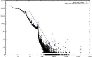
Figure 1: Left: the degree distribution of our graph. Right: the execution time (in minutes) as a function of the number of vertices considered as high degree ones.

We plot in Figure 1 (right) the running time of Algorithm 8 (new-vertex-listing) as a function of the number of vertices with degree larger than $K$, for varying values of $K$. Surprisingly enough, this plot shows clearly that the time performance increases drastically as soon as a few vertices are considered as high degree ones. This may be seen as a consequence of the fact that edge-iterator is very efficient when the maximal degree is bounded; managing high degree vertices efficiently with Algorithm 8 (new-vertex-listing) and then the low degree ones with edge-iterator therefore leads to good performances. In other words, the few high degree vertices (which may be observed on the degree distribution plotted in Figure 1) are responsible for the low performance of edge-iterator.

When $K$ decreases, the number of vertices with degree larger than $K$ increases, and the performances continue to be better and better for a while. They reach a minimal running time, and then the running time grows again. The other important point here is that this growth is very slow, and thus the performance of the algorithm remains close to its best for a wide range of values of $K$. This implies that, with any reasonable guess for $K$, the algorithm performs well.

7 Conclusion.

In this contribution, we gave a detailed survey of existing results on triangle problems, and we completed them in two directions. First, we gave the space complexity of each previously known algorithm. Second, we proposed new algorithms that achieve both optimal time complexity and low space needs. Taking space requirements into account is a key issue in this context, since this currently is the bottleneck for triangle problems when the considered graphs are very large. This is discussed on a practical case in Section 6, where we show that our compact algorithms make it possible to handle cases that were previously out of reach.

Another significant contribution of this paper is the analysis of algorithm performances on power-law graphs (Section 5), which model a wide variety of very large graphs met in practice. We were able to show that, on such graphs, several algorithms have better performance than in the general (sparse) case.

Finally, the current state of the art concerning triangle problems, including our new results, may be summarized as follows:

• except the fact that pseudo-listing may have a $\Theta(n)$ space overhead (depending on the underlying algorithm), there is no known difference in time and space complexities between finding, counting, and pseudo-listing;

• the fastest known algorithms for these three problems rely on matrix product and are in $O(n^{2.376})$ time and $\Theta(n^{2})$ space (Theorem 1), or in $O(m^{1.41})$ time and $O(m^{1.185})$ space (Theorem 2); however, no lower bound better than the trivial $\Omega(m)$ one is known for the time complexity of these problems;

• the other known algorithms rely on solutions to the listing problem and have the same performances as on this problem; they are slower than matrix approaches but need less space;

• listing can be solved in $\Theta(n^{3})$ or $\Theta(n\cdot m)$ (optimal in the general case) time and $\Theta(1)$ (optimal) space (Theorems 4, 5 and 6); this can be achieved from a sorted simple compact representation of the graph;

• listing may also be solved in $\Theta(m^{\frac{3}{2}})$ (optimal in the general and sparse cases) time and $\Theta(n)$ space (Theorems 13 and 11), still from a simple compact representation of the graph; this is much better for sparse graphs;

• in the case of power-law graphs, it is possible to prove better complexities, leading to $O(m\cdot n^{\frac{1}{\alpha}})$ time and $\Theta(n)$ space solutions, where $\alpha$ is the exponent of the power-law (Theorem 15);

• in practice, it is possible to obtain very good performances (both concerning time and space needs) using Algorithm 9 (new-listing) and Algorithm 7 (compact-forward).

We detailed several other results, but they are weaker (they need the adjacency matrix of the graph in input and/or have higher complexities) than these ones.

This contribution also opens a set of questions for further research, most of them related to the tradeoff between space and time efficiency. Let us cite for instance:

• can matrix approaches be modified in order to induce less space complexity?

• is listing feasable in $o(n)$ space, while still in optimal time $\Theta(m^{\frac{3}{2}})$?

• is it possible to design a listing algorithm with complexity $o(m\cdot n^{\frac{1}{\alpha}})$ time and $o(n)$ space for power-law graphs with exponent $\alpha$? what is the optimal time complexity in this case?

It is also important to notice that other approaches exist, based for instance on streaming algorithmics (avoiding to store the graph in central memory) [22, 4, 24] and/or approximate algorithms [31, 24, 34], and/or various methods to compress the graph [8, 9]. These approaches are very promising for graphs even larger than the ones considered here, in particular the ones that do not fit in central memory.

Another interesting approach would be to express the complexity of triangle algorithms in terms of the number of triangles in the graph (and of its size). Indeed, it may be possible to achieve much better performance for listing algorithms if the graph contains few triangles. Likewise, it is reasonable to expect that triangle listing, but also pseudo-listing and counting, may perform poorly if there are many triangles in the graph. The finding problem, on the contrary, may be easier on graphs having many triangles. To our knowledge, this direction has not yet been explored.

Finally, the results we present in Section 5 take advantage of the fact that most very large graphs considered in practice may be approximed by power-law graphs. It is not the first time that algorithms for triangle problems use underlying graph properties to get improved performance. For instance, results on planar graphs are provided in [23], and results using arboricity in [14, 3]. It however appeared quite recently that many large graphs met in practice have some nontrivial (statistical) properties in common, and using these properties in the design of efficient algorithms still is at its very beginning. We consider this as a key direction for further research.

Acknowledgments. I warmly thank Frédéric Aidouni, Michel Habib, Vincent Limouzy, Clémence Magnien, Thomas Schank and Pascal Pons for helpful comments and references. I also thank Paolo Boldi from the WebGraph project [10], who provided the data used in Section 6. This work was partly funded by the MetroSec (Metrology of the Internet for Security) [39] and PERSI (Programme d’Étude des Réseaux Sociaux de l’Internet) [40] projects.

References

- [1] R. Albert and A.-L. Barabási. Statistical mechanics of complex networks. Reviews of Modern Physics, 74, 47, 2002.
- [2] Noga Alon, Raphael Yuster, and Uri Zwick. Finding and counting given length cycles. In European Symposium Algorithms (ESA), 1994.
- [3] Noga Alon, Raphael Yuster, and Uri Zwick. Finding and counting given length cycles. Algorithmica, 17(3):209223, 1997.
- [4] Ziv Bar-Yossef, Ravi Kumar, and D. Sivakumar. Reduction in streaming algorithms with an application of counting triangles in graphs. In ACM/SIAM Symposium On Discrete Algorithms (SODA), 2002.
- [5] Vladimir Batagelj. Personnal communication, 2006.
- [6] Vladimir Batagelj and Andrej Mrvar. Pajek: A program for large network analysis. Connections, 21(2):4757, 1998.
- [7] Vladimir Batagelj and Andrej Mrvar. A subquadratic triad census algorithm for large sparse networks with small maximum degree. Social Networks, 23:237–243, 2001.
- [8] P. Boldi and S. Vigna. The webgraph framework i: compression techniques. In WWW, 2004.
- [9] P. Boldi and S. Vigna. The webgraph framework ii: Codes for the world-wide web. In DCC, 2004.
- [10] Paolo Boldi. WebGraph project. http://webgraph.dsi.unimi.it/.
- [11] Paolo Boldi, Bruno Codenotti, Massimo Santini, and Sebastiano Vigna. Ubicrawler: a scalable fully distributed web crawler. Softw., Pract. Exper., 34(8):711–726, 2004.
- [12] Béla Bollobás and Oliver M. Riordan. Handbook of Graphs and Networks: From the Genome to the Internet, chapter Mathematical results on scale-free random graphs. Wiley-VCH, 2002.
- [13] U. Brandes and T. Erlebach, editors. Network Analysis: Methodological Foundations. LNCS, Springer-Verlag, 2005.
- [14] Norishige Chiba and Takao Nishizeki. Arboricity and subgraph listing algorithms. SIAM Journal of Computing, 14, 1985.
- [15] R. Cohen, R. Erez, D. ben Avraham, and S. Havlin. Reply to the comment on ’breakdown of the internet under intentional attack’. Phys. Rev. Lett, 87, 2001.
- [16] Don Coppersmith and Shmuel Winograd. Matrix multiplication via arithmetic progressions. J. Symb. Comput., 9(3):251–280, 1990.
- [17] Thomas H. Cormen, Charles E. Leiserson, Ronald L. Rivest, and Clifford Stein. Introduction to Algorithms, Second Edition. MIT Press, 2001.
- [18] S.N. Dorogovtsev and J.F.F. Mendes. Comment on ’breakdown of the internet under intentional attack’. phys. Rev. Lett, 87, 2001.
- [19] Stephen Eubank, V.S. Anil Kumar, Madhav V. Marathe, Aravind Srinivasan, and Nan Wang. Structural and algorithmic aspects of massive social networks. In ACM/SIAM Symposium on Discrete Algorithms (SODA), 2004.
- [20] Frank Harary and Helene J. Kommel. Matrix measures for transitivity and balance. Journal of Mathematical Sociology, 1979.
- [21] Frank Harary and Herbert H. Paper. Toward a general calculus of phonemic distribution. Language : Journal of the Linguistic Society of America, 33:143169, 1957.
- [22] Monika Rauch Henzinger, Prabhakar Raghavan, and Sridar Rajagopalan. Computing on data streams. Technical report, DEC Systems Research Center, 1998.
- [23] Alon Itai and Michael Rodeh. Finding a minimum circuit in a graph. SIAM Journal on Computing, 7(4):413423, 1978.
- [24] H. Jowhari and M. Ghodsi. New streaming algorithms for counting triangles in graphs. In COCOON, 2005.
- [25] Matthieu Latapy. Triangle computation web page. http://www.liafa.jussieu.fr/~latapy/Triangles/.
- [26] Matthieu Latapy and Clémence Magnien. Measuring fundamental properties of real-world complex networks, 2006. Submitted.
- [27] J. Leskovec, J. Kleinberg, and C. Faloutsos. Graphs over time: Densification laws, shrinking diameters and possible explanations. In ACM SIGKDD, 2005.
- [28] Ron Milo, Shai Shen-Orr, Shalev Itzkovitz, Nadav Kashtan, Dmitri Chklovskii, and Uri Alon. Network motifs: Simple building blocks of complex networks. Science, 298:824827, 2002.
- [29] Burkhard Monien. How to find long paths efficiently. Annals of Discrete Mathematics, 25:239–254, 1985.
- [30] C.R. Edling P. Holme and F.Liljeros. Structure and time-evolution of an internet dating community. Social Networks, 26(2), 2004.
- [31] Thomas Schank and Dorothea Wagner. Approximating clustering coefficient and transitivity. Technical report, Universität Karlsruhe, Fakultät für Informatik, 2004.
- [32] Thomas Schank and Dorothea Wagner. Finding, counting and listing all triangles in large graphs. Technical report, Universität Karlsruhe, Fakultät für Informatik, 2005.
- [33] Thomas Schank and Dorothea Wagner. Finding, counting and listing all triangles in large graphs, an experimental study. In Workshop on Experimental and Efficient Algorithms (WEA), 2005.
- [34] Asaf Shapira and Noga Alon. Homomorphisms in graph property testing - a survey. In Electronic Colloquium on Computational Complexity (ECCC), 2005.
- [35] Duncan J. Watts and Steven H. Strogatz. Collective dynamics of smallworld networks. Nature, 393:440–442, 1998.
- [36] Esti Yeger-Lotem, Shmuel Sattath, Nadav Kashtan, Shalev Itzkovitz, Ron Milo, Ron Y. Pinter, and Uri Alon andHanah Margalit. Network motifs in integrated cellular networks of transcription-regulation and protein-protein interaction. Proc. Natl. Acad. Sci. USA 101, 59345939, 2004.
- [37] Raphael Yuster and Uri Zwick. Detecting short directed cycles using rectangular matrix multiplication and dynamic programming. In ACM/SIAM Symposium On Discrete Algorithms (SODA), pages 254–260, 2004.
- [38] Raphael Yuster and Uri Zwick. Fast sparse matrix multiplication. In European Symposium on Algorithms (ESA), pages 604–615, 2004.
- [39] Metrosec project. http://www2.laas.fr/METROSEC/.
- [40] Persi project. http://www.liafa.jussieu.fr/~persi/.