Measuring Fundamental Properties of
Real-World Complex Networks

Abstract

Complex networks, modeled as large graphs, received much attention during these last years. However, data on such networks is only available through intricate measurement procedures. Until recently, most studies assumed that these procedures eventually lead to samples large enough to be representative of the whole, at least concerning some key properties. This has crucial impact on network modeling and simulation, which rely on these properties.

Recent contributions proved that this approach may be misleading, but no solution has been proposed. We provide here the first practical way to distinguish between cases where it is indeed misleading, and cases where the observed properties may be trusted. It consists in studying how the properties of interest evolve when the sample grows, and in particular whether they reach a steady state or not.

In order to illustrate this method and to demonstrate its relevance, we apply it to data-sets on complex network measurements that are representative of the ones commonly used. The obtained results show that the method fulfills its goals very well. We moreover identify some properties which seem easier to evaluate in practice, thus opening interesting perspectives.

1 Context.

Complex networks of many kinds, modeled as large graphs, appear in various contexts. In computer science, let us cite internet maps (at IP, router or AS levels, see for instance [23, 26, 19, 1]), web graphs (hyperlinks between pages, see for instance [33, 16, 11, 12, 5]), or data exchanges (in peer-to-peer systems, using e-mail, etc, see for instance [30, 50, 39, 29]). One may also cite many examples among social, biological or linguistic networks, like co-authoring networks, protein interactions, or co-occurrence graphs for instance.

It appeared recently (at the end of the 90s [51, 23, 33, 7, 16]) that most real-world complex networks have nontrivial properties which make them very different from the models used until then (mainly random, regular, or complete graphs and ad hoc models). This lead to the definition of a set of statistics, the values of which are considered as fundamental properties of the complex network under concern. This induced in turn a stream of studies aimed at identifying more such properties, their causes and consequences, and capturing them into relevant models. They are now used as key parameters in the study of various phenomena of interest like robustness [8, 32], spreading of information or viruses [46, 25], and protocol performance [41, 30, 50, 29] for instance. They are also the basic parameters of many network models and simulation systems, like for instance brite [42]. This makes the notion of fundamental properties of complex networks a key issue for current research in this field. For recent surveys on typical properties and related issues, see for instance [15, 14].

However, most real-world complex networks are not directly available: collecting data about them requires the use of a measurement procedure. In most cases, this procedure is an intricate operation that gives a partial and possibly biased view. Most contributions in the field then rely on the following (often implicit) assumption: during the measurement procedure, there is an initial phase in which the collected data may not be representative of the whole, but when the sample grows one reaches a steady state where the fundamental properties do not vary anymore. Authors therefore grab a large amount of data (limited by the cost of the measurement procedure, and by the ability to manage the obtained data) and then suppose that the obtained view is representative of the whole, at least concerning these properties.

Until recently, very little was known on the relevance of this approach, which remains widely used (because in most case there is no usable alternative method). This has long been ignored, until the publication of some pioneering contributions [35, 10] showing that the bias induced by measurement procedures is significant, at least in some important cases. It is now a research topic in itself, with both theoretical, empirical and experimental studies; see for instance [35, 10, 6, 28, 20] . In this stream of studies, the authors mainly try to identify the impact of the measurement procedure on the obtained view and to evaluate the induced bias. The central idea, first introduced in [35, 10], is to take a graph $G$ (generally obtained from a model or a real-world measurement), simulate a measurement of $G$ thus obtaining the view $G^{\prime}$ and compare $G$ and $G^{\prime}$. This gave rise to significant insight on complex network metrology, but much remains to be done.

2 Approach and scope.

Our contribution belongs to the current stream of studies on real-world complex networks, and more precisely on the measurement of these networks. It addresses the issue of the estimation of their basic properties, with the aim of providing a practical solution to this issue. Indeed, until now, authors studying real-world complex networks had no choice but to follow the classical assumption that their sample is large enough to be representative of the whole, even though this has been proved to be far from obvious [35, 10, 6, 28, 20]. We will make it possible to evaluate the relevance of this classical assumption in practical cases.

We notice that the vast majority of real-world complex network studies rely on samples obtained through a measurement procedure that is interrupted when the obtained sample is considered large enough to be representative of the whole. Then, we mimic this by processing very large measurements of real-world complex networks: we study what the observed properties would be if one had stopped the measurement when the sample had reached a given size, smaller than the final one.

The main strength of this approach is that it relies on real measurements of complex networks, while previous works had to model the complex network under concern, the measurement process, or both, see for instance [35, 6, 28, 20]. Such a modeling is a challenging task since the measurement procedure generally is intricate, and since we do not know the underlying complex network that we actually measure. We avoid these problems here since we rely on real-world data, obtained in a way that is representative of what is done in practice.

This also means that measuring the same complex networks but in another way, and/or measuring other complex networks, may lead to different results. This is why we paid high attention to use measurements that are representative of the ones commonly used, and come from four very different contexts (see Section 3); this reduces the risk of results specific to one case. In each of these contexts, we moreover used several measurements (of different sizes, conducted at different times, and/or with significantly different methods); all the results were consistent and we present here one typical example for each case. Notice also that we provide the programs we used here, which makes it possible to conduct the same analysis on any measurement data-set [2].

Before turning to the description of our data-sets and entering in the core of this contribution, let us emphasize a few key points.

$\bullet$ Though we use real-world data in our study, we do not seek results on these particular examples. It makes no doubt that studying them in depth would also be relevant, and that our observations raise interesting issues on each particular case, but this is not our concern here. We only consider them as typical large-scale measurements which we use to illustrate our approach.

$\bullet$ Likewise, we will not discuss the measurement procedures themselves, which may vary and may be improved; the key point is that these measurements are representative of the ones used in current research. In particular, we follow the classical convention consisting in ignoring the bias induced by the fact that the complex network under concern may evolve during the measurement. This is an important and interesting issue, but it is out of the scope of this paper.

$\bullet$ It must also be clear that handling such graphs, together with their evolution, is an algorithmic challenge. It does not only force us to use important capacities in central memory and in processing power: algorithms with a time or space cost more than linear in the number of nodes $n$ and/or links $m$ are almost unusable in this context . We will therefore carefully choose the algorithms we use in our computations, and discuss their complexities all along the paper .

3 Method and data-sets.

To achieve our goal, we need data in the following form: given a real-world complex network measurement, for each integer $n$ we need the graph one would obtain if this measurement had been stopped as soon as $n$ nodes had been discovered. We then compute the properties under concern for each of these graphs, obtaining plots of their value as a function of the sample size $n$ .

Our data-sets are derived from raw data on how complex networks are measured, which we describe below. They come from some of the largest and highest quality data-sets currently available, and span quite well the variety of complex networks usually considered in computer science. From this raw data, we first extracted, for each node and link, the time at which it was discovered . Then we wrote a program that runs through this stream of node and link arrivals (ordered by the time at which they are discovered) until the sample reaches the prescribed size $n$, and then computes the desired statistics.

Because these data-sets and the program may be useful for other purpose, and because they are needed to reproduce our results, we provide them at [2].

We recall that we only use these data-sets as examples here; discussing the relevance of such graphs and their particular properties is out of the scope of this paper. The key point is that they are representative of what is used in most studies, and that in most cases they are significantly larger. It means that most known results on these objects are actually derived from samples lying somewhere between the beginning and the end of the measurement in our cases.

3.0.1 The inet data-set.

This data-set comes from the Skitter project at caida [1]. Several machines scattered around the world run traceroute-like probes to a list of almost $1\,000\,000$ destinations, on an approximately daily basis. They record each route discovered this way, together with the time at which the probe was launched (and additional information that we do not need here). They make this data freely available for academic research.

Such measurements are often used to construct maps of the internet at IP, router or AS levels. The IP maps are nothing but the set of all IP addresses viewed during the measurement, with a link between any two of them if they are neighbors on a collected path. Obtaining router or AS maps from such data is a challenge in itself, and subject to some error, see for instance [19]. Here we will simply consider the IP level.

We downloaded all the data collected by Skitter from january 2005 to may 2006. During this period, $20$ machines ran probes with no interruption (other experienced interruptions, thus we did not include them), leading to $4\,616\,234\,615$ traceroute-like records, and approximately $350$ gigabytes of compressed data. We assumed that the links corresponding to a given route were seen at the time (in seconds) the probing of this route was started.

The graph finally obtained contains $1\,719\,037$ nodes and $11\,095\,298$ links.

3.0.2 The web data-set.

Web graphs, i.e. sets of web pages identified by their URL and hyper-links between them, are often used as typical examples of complex networks. Indeed, it is quite easy to get large such graphs using a crawl: from a set of initial pages (possibly just one), one follows its links and iterates this in a breadth-first manner. Collecting huge such graphs however is much more difficult, since several reasons like limitations in computing capabilities and crawling policies lead to many technical constraints.

Here we used a data-set provided by one of the current leading projects on web crawling and management, namely WebGraph [11, 12, 5]. Their crawler is one of the most efficient currently running, and their data-sets on web graphs are the largest available ones. They provided us with a web graph of pages in the .uk domain containing $39\,459\,925$ nodes (web pages) and $921\,345\,078$ directed links (not including loops). Moreover, they provided us with the time at which each page was visited (each was visited only once), thus at which each node and its outgoing links were discovered. This crawl has been ran from the 11-th of July, 2005, at 00:51, to the 30-th at 23:24, leading to almost 20 days of measurement. The time precision is $1$ minute.

From this data, we obtained a final graph with $39\,459\,925$ nodes and $783\,027\,125$ undirected links  with the time (in minutes) at which they were discovered.

3.0.3 The p2p data-set.

Several recent studies use traces of running peer-to-peer file exchange systems to give evidence of some of their properties, and then design efficient protocols, see for instance [30, 50, 29]. They often focus on user behaviors or data properties, and the complex network approach has proved to be relevant in this context. Collecting such data however is particularly challenging because of the distributed and dynamic nature of these systems. Several approaches exist to obtain data on these exchanges, among which the capture of the queries processed by a server in a semi-centralized system.

We used here data obtained this way: it contains all the queries processed by a large eDonkey server running the Lugdunum software [3]. The trace begins from a reboot of the server, on the 8-th of may, 2004, and lasts until the 10-th, leading to more than $47$ hours of capture with a time precision of $1$ second. During this period, the server processed $215\,135\,419$ user commands (logins, logouts and search queries). Here, we kept the search queries, of the following form: $T\ Q\ F\ S_{1}\ S_{2}\ \dots\ S_{n}$, where $T$ is the time at which this query was treated, $Q$ is the peer which sent this query, $F$ is the queried file, and $S_{1}$, $S_{2}$, $\dots$, $S_{n}$ is a list of possible providers for this file (they declared to the server that they have it) sent to $Q$ by the server (so that $Q$ may contact them directly to get the file). The trace contains $212\,086\,691$ such queries.

We constructed the exchange graph, obtained from this data by considering that, for each query, at time $T$, the links between $Q$ and $S_{i}$ appear for each $i$. This graph captures some information on exchanges between peers, which is commonly used as a reasonable image of actual exchanges, see for instance [29, 39]. The final exchange graph we obtained has $5\,792\,297$ nodes and $142\,038\,401$ links.

3.0.4 The ip data-set.

Since a few years, it has appeared clearer and clearer that measuring the way computer networks (and their users) behave in running environments is essential. This is particularly true for the internet, where very little is known on large-scale phenomena like end-to-end traffic or anomalies (congestions, failures, attacks, etc). In this spirit, several projects measure and study internet traffic, see for instance [36, 37, 4].

Here we obtained from the MetroSec project [4] the following kind of traces. They record the headers of all IP packets managed by some routers during the capture period of time. The trace we use here consists in a capture done on the router at the interface between a large laboratory [34] and the outside internet, between March 7-th, 08:10 am, and March 15-th, 2006, 02:22 pm, leading to a trace of a little more than 8 days and $709\,270\,078$ recorded IP headers. The trace contains the time at which the packet was managed by the router, with a precision of $10^{-6}$ second.

From this trace, we extracted for each IP header the sender and target of the packet, together with the time at which this packet was routed. We thus obtained the graph in which nodes are IP addresses and each link represents the fact that the corresponding IP addresses exchanged (at least) one packet. Such graphs are used (often implicitely) to study the properties of exchanges, to seek attack traces, etc. See for instance [36]. The final graph used here has $2\,250\,498$ nodes and $19\,394\,216$ links.

4 Analysis

In this section, we present our results on the data-sets described above. Our aim is to span the main basic properties classically observed on real-world complex networks. For each set of properties we recall the appropriate definitions, we discuss their computation and we analyze their evolution with the size of the sample in each of our four cases. The key point is that we compare these behaviors to the classical assumptions in the field.

In all the definitions in this section, we suppose that a graph $G=(V,E)$ is given, and we denote by $n=|V|$ its number of nodes, by $m=|E|$ its number of links, and by $N(v)=\{u\in V,\ (v,u)\in E\}$ the set of neighbors, or neighborhood, of node $v$. We consider here undirected graphs (we make no distinction between $(u,v)$ and $(v,u)$) since most classical properties are defined on such graphs only. Moreover, recall that our graphs have no loop and no multiple links, see Section 2.

In order to give precise space and time complexities, we need to make explicit how we will store our graphs in central memory. We will use the sorted adjacency arrays encoding: for each $v\in V$ we store $N(v)$ in a sorted array, together with its size $|N(v)|$, and access to these informations is granted in $\Theta(1)$ time and space. This encoding ensures that the graph is stored in space $\Theta(m)$ and that the presence of any link can be tested in $\Theta(\log(n))$ time and $\Theta(1)$ space.

4.1 Basic facts.

4.1.1 Size evolution during time.

As already discussed, in all the paper the properties we consider will be observed as functions of the sample size, which is the classical parameter in complex network studies. However, it would also be relevant to discuss the evolution of these properties during time . The plots in Figure 1 give the relation between the two.

Figure 1: Evolution of the number of nodes and links during time (in hours). From left to right and top to bottom: inet, p2p, web and ip graphs.

It appears clearly on these plots that in none of the four cases does the measurement reach a state where it discovers no or few new nodes and links. Instead, the size of the obtained sample is still growing significantly by the end of the measurement. This means that, even for huge measurements like the ones we consider, the final result probably is far from a complete view of the network under concern. In other words, it is not possible to collect complete data on these networks in reasonable time and space, at least using such measurements.

This implies that the observed properties are those of the samples, and may be different from the ones of the whole network even at the end of the measurement. To this regard, an important issue of this contribution is to determine whether this is the case or not, and more precisely, if used samples are representative of what one would obtain with larger samples or not.

Another important observation is that, in all cases, the number of links $m$ grows significantly faster than the number of nodes $n$. We will deepen this in Section 4.2.

Finally, notice that in the case of inet the measurement discovers a huge number of nodes and links (roughly half the nodes discovered at the end of the measurement) very quickly. This is due to the measurement method (based on traceroute-like probes) and should not be considered as a surprising fact (it corresponds to the first probe from each source to each destination). This will have an influence on the plots in the rest of the paper: the first half of each plot will correspond to a very short measurement time. One may notice that many studies rely on measurement that do only one probe per destination, thus leading to samples which may be compared to the ones in the first halves of our plots. However, as already explained, discussing this is out of the scope of this contribution.

4.1.2 Connectivity.

A connected component of a graph is a maximal (no node can be added) set of nodes such that a path exists between any pair of nodes in this set. The connected components and their sizes are computed using a graph traversal (like a breadth-first search) in $\Theta(n)$ space and $\Theta(m)$ time.

In most real-world complex networks, it has been observed that there is a huge connected component, often called giant component, together with a number of small components containing no more than a few percents of the nodes, often much less, if any.

Figure 2: Fraction of nodes in the largest connected component as a function of the sample size, with an inset zoom on the last three quarters of each plot. From left to right and top to bottom: inet, p2p, web and ip graphs.

Figure 3: Number of connected components as a function of the sample size. From left to right and top to bottom: inet, p2p, web and ip graphs.

In the four cases studied here, these observations are confirmed, and this is very stable independently of the size of the sample. This is visible in Figure 2 where we plot the proportion of nodes in the giant component: it is very close to $1$ in all the cases, even for quite small samples (the only noticable thing is that up to $7\,\%$ of the nodes in p2p are not in the giant component, but it still contains more than $92\,\%$ of them). On the contrary, the number of connected components varies depending on the case, as well as its behavior as a function of the size of the graph, see Figure 3. Since there is no classical assumption concerning this, and no clear general behavior, we do not detail these results here.

4.2 Average degree and density.

The degree $d^{o}(v)$ of a node $v$ is its number of links, or, equivalently, its number of neighbors: $d^{o}(v)=|N(v)|$. The average degree $d^{o}$ of a graph is the average over all its nodes: $d^{o}=\frac{1}{n}\sum_{v}d^{o}(v)$. The density is the number of links in the graph divided by the total number of possible links: $\delta=\frac{2\cdot m}{n\cdot(n-1)}$. The density indicates up to what extent the graph is fully connected (all the links exist). Equivalently, it gives the probability that two randomly chosen nodes are linked in the graph. There is a trivial relation between the average degree and the density: $d^{o}=\delta\cdot(n-1)$. Both the average degree and the density are computed in $\Theta(n)$ time and $\Theta(1)$ space.

The average degree of complex networks is supposed to be small, and independent of the sample size, as soon as the sample is large enough. This implies that the density $\delta$ is supposed to go to zero when the sample grows, since $\delta=\frac{d^{o}}{n-1}$.

It appears in Figures 4 and 5 that the average degree is indeed very small compared to its maximal possible value, and that the density is close to zero, as expected.

Figure 4: Average degree as a function of the sample size. From left to right and top to bottom: inet, p2p, web and ip graphs.

Figure 5: Density as a function of the sample size, together with inset zooms of the rightmost halves of the plots. From left to right and top to bottom: inet, p2p, web and ip graphs.

In the cases of web and ip, the measurement reaches a regime in which the average degree is rather stable (around $40$ and $17$, respectively), and equivalently the density goes to $0$. This means that there is little chance that this value will evolve if the sample grows any further, and that the observed value would be the same independently of the sample size (as long as it is not too small). In this sense, the observed value may be trusted, and at least it is not representative of only one particular sample. We will discuss this further in Section 5.

In the two the other cases, inet and p2p, the observed average degree is far from constant, and the density does not go to zero. This has a strong meaning: in these cases, one cannot consider the value observed for the average degree on any sample as significant. Indeed, taking a smaller or a larger sample would lead to a different value. Since the measurements we use here are already huge, this even means that there is little chance that the observed value will reach a steady state within reasonable time using such measurements. We will discuss this further in Section 5.

Going further, one may observe that in some cases the number of links $m$ grows faster than the number of nodes $n$ (the average degree grows), and even as $n^{2}$ (the density is stable) in some parts of the plots. In order to deepen this, we present the plots of $m$ as a function of $n$ in Figure 6, in log-log scales: straight lines indicate that $m$ evolves as a power of $n$, the exponent being the slope of the line.

Figure 6: Number of links as a function of the number of nodes in log-log scales, together with the plots of $y=x$ and $y=x^{2}$ (with an appropriate shift). From left to right and top to bottom: inet, p2p, web and ip graphs.

Such plots have been studied in the context of dynamic graphs [40]. In this paper, the authors observe that $m$ seems to evolve as a power of $n$, and that the average degree grows with time, which was also observed in [21]. In our context, the behavior of $m$ as a function of $n$ is quite different: the plots in Figure 6 are far from straight lines in most cases. This means that exploring more precisely the relations between $m$ and $n$ needs significantly more work, which is out of the scope of this paper. The key point here is that, in some cases, $m$ grows faster than $n$, and that the classical algorithmic assumption that $m\in\Theta(n)$ is not always true.

Finally, the properties observed in this section are in sharp contradiction with the classical assumptions of the field for two of our four real-world cases (inet and p2p). This means that, in these cases, one cannot assume that the average degree observed with such a measurement is representative of the one of the actual network: taking a larger or smaller sample leads to significantly different estimations. In the two other cases (web and ip), instead, the measurement seems to reach a state where the observed values are significant.

4.3 Average distance and diameter.

We denote by $d(u,v)$ the distance between $u$ and $v$, i.e. the number of links on a shortest path between them. We denote by $d(u)=\frac{1}{n}\sum_{v}d(u,v)$ the average distance from $u$ to all nodes, and by $d=\frac{1}{n}\sum_{u}d(u)=\frac{1}{n^{2}}\sum_{u,v}d(u,v)$ the average distance in the considered graph. We also denote by $D=\max_{u,v}d(u,v)$ the diameter of the graph, i.e. the largest distance.

Notice that the definitions above make sense only for connected graphs. In practice, one generally restricts the computations to the largest connected component, which is reasonable since the vast majority of nodes are in this component (see Section 4.1.2). We will follow this convention here; therefore, in the rest of this subsection, the graph is supposed to be connected (i.e. it has only one connected component) and the computations are made only on the giant component of our graphs.

4.3.1 Computation.

Computing distances from one node to all the others in an undirected unweighted graph can be done in $\Theta(m)$ time and $\Theta(n)$ space with a breadth-first search (BFS). One then obtains all the distances in the graph, needed for exact average distance and diameter computations, in $\Theta(n\cdot m)$ time and $\Theta(n)$ space. This is space efficient, but not fast enough for our purpose (see Section 2). Faster algorithms have been proposed [9, 49, 24], but they all have a $\Theta(n^{2})$ space cost, which is prohibitive in our context. See [52] for a survey, and [45, 22] for recent results on the topic.

Despite this, the average distance and the diameter are among the most classical properties used to describe real-world complex networks. Therefore, computing accurate estimations of the average distance and the diameter is needed, and much work has already be done to this regard [52, 45, 22].

A classical approach is to approximate the average distance by using a limited number of BFS and then average over this sample. See [22] for formal results on this. We used here a variant of this approach: at step $i$ we choose a random node, say $v_{i}$, and we compute its average distance to all other nodes, $d(v_{i})$, in time $\Theta(m)$ and space $\Theta(n)$. Then we compute the $i$-th approximation of the average distance as $d_{i}=\frac{1}{i}\sum_{j=1}^{i}d(v_{j})$. The loop ends at the first $i>i_{\min}$ such that the variations in the estimations have been less than $\epsilon$ during the last $i_{\min}$ steps, i.e. $|d_{j+1}-d_{j}|<\epsilon$, for all $j,i-i_{\min}\leq j<i$. The variables $i_{\min}$ and $\epsilon$ are parameters used to ensure that at least $i_{\min}$ iterations are processed, and that the variation during the $i_{\min}$ last iterations is no more than $\epsilon$. In all the computations below, we took $i_{\min}=10$ and $\epsilon=0.1$.

Such approaches are much less relevant for notions like the diameter, which is a worst case notion: by computing the worst case on a sample, one may miss a significantly worse case. Instead, we propose simple and efficient algorithms to find lower and upper bounds for the diameter.

First notice that the diameter of a graph is at least the height of any BFS tree of this graph. Going further, it is shown in [18, 17] that the following algorithm finds excellent approximations of the diameter of graphs in some specific cases: given a randomly chosen node $v$, one first finds the node $u$ which is the further from $v$ using a BFS, and then processes a new BFS from $u$; then the lower bound obtained from $u$ is at least as good as the one obtained from $v$, and is very close to the diameter for some graph classes.

Now, notice that the diameter of a graph cannot be larger than the diameter of any of its (connected) subgraphs, in particular of its BFS trees. Therefore the diameter is bounded by the largest distance in any of its BFS trees, which can be computed in $\Theta(n)$ time and space, once the BFS tree is given. One then obtains an upper bound for the diameter in the graph.

We finally iterate the following to find accurate bounds for the diameter. Randomly choose a node and use it to find a lower bound using the algorithm described above; then choose a node in decreasing order of degrees and use it to find an upper bound as described above. In the latter, nodes are chosen in decreasing order of their degrees because high degree nodes intuitively lead to BFS trees with smaller diameter. We iterate this at least $10$ times, and until the difference between the two bounds becomes lower than $5$. In the vast majority of the cases considered here, the $10$ initial steps are sufficient. Since each step needs only $\Theta(m)$ time and $\Theta(n)$ space, the overall algorithm performs very well in our context.

4.3.2 Usual assumptions and results.

It appeared in various contexts (see for instance [51, 33, 7, 16]) that the average distance and the diameter of real-world complex networks is much lower than expected, leading to the so-called small-world effect: any pair of nodes tends to be connected by very short paths. Going further, both quantities are also supposed to grow slowly with the number of nodes $n$ in the graph (like its logarithm or even slower).

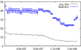
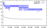
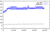
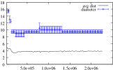
Figure 7: Estimation of the average distance and bounds for the diameter, as a function of the sample size. From left to right and top to bottom: inet, p2p, web and ip graphs.

Figure 7 shows several things. First, the obtained bounds for the diameter are very tight and give a precise information on its actual value. The heuristics described above therefore are very efficient and provide a good alternative to previous methods in our context. These plots also indicate that our approximation of the average distance is consistent: if the randomly chosen nodes had a significant impact on our evaluation, then the corresponding plots would not be smooth.

Concerning the obtained values themselves, they clearly confirm that both the average distance and the diameter are very small compared to the size of the graphs. However, their evolution is in sharp contrast with the usual assumptions in the case of inet and ip: both the average distance and the diameter are stable or even decrease  with the size of the sample in these cases (with a sharp increase at the end for the diameter of inet). In the case of web, however, the observed behavior fits very well classical assumptions. The situation is not so clear for ip: the values seem stable, but they may grow very slowly.

These surprising observations may have a simple explanation. Indeed, the usual assumptions concerning average distance and diameter are strongly supported by the fact that the average distance and diameter of various random graphs (used to model complex networks) grow with their size. However, in these models, the average degree $d^{o}$ generally is supposed to be a constant independent of the size. If it is not, then the average distance in these graphs typically grows as $\frac{\log(n)}{\log(d^{o})}$ [13, 44]. This means that, if $d^{o}$ grows with $n$ as observed in Section 4.2, it is not surprising that the average distance and the diameter are stable or decrease. Likewise, in the case of web where the average degree is constant, the average distance and the diameter should increase slowly, which is in accordance with our observations.

4.4 Degree distribution.

The degree distribution of a graph is the proportion $p_{k}$ of nodes of degree exactly $k$ in the graph, for all $k$. Given the encoding we use, its computation is in $\Theta(n)$ time and space.

Degree distributions may be homogeneous (all the values are close to the average, like in Poisson and Gaussian distributions), or heterogeneous (there is a huge variability between degrees, with several orders of magnitude between them). When a distribution is heterogeneous, it makes sense to try to measure this heterogeneity rather than the average value. In some cases, this can be done by fitting the distribution by a power-law, i.e. a distribution of the form $p_{k}\sim k^{-\alpha}$. In such cases, the exponent $\alpha$ may be considered as an indicator of how heterogeneous the distribution is.

4.4.1 Usual assumptions and results.

Degree distributions of complex networks have been identified as a key property since they are very different from what was thought until recently [23, 33], and since it was proved that they have a crucial impact on phenomena of high interest like network robustness [8, 32] or diffusion processes [46, 25]. They are considered to be highly heterogeneous, generally well fitted by a power-law, and independent of the size of the graph.

We first present in Figure 8 the degree distributions observed in our four cases at the end of the measurement procedure. These plots confirm that the degrees are very heterogeneous, with most nodes having a low degree ($49\%$, $39\%$, $24\%$ and $93\%$ have degree lower than $5$ in inet, p2p, web and ip respectively), but some nodes having a very high degree (up to $35\,455$, $15\,115$, $1\,776\,858$ and $259\,905$ in inet, p2p, web and ip). We however note that the p2p degree distribution does not have a heavy tail, but rather an exponential cutoff. All the degree distributions are reasonably, but not perfectly, fitted by power laws on several decades.

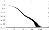
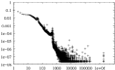
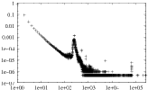
Figure 8: Degree distributions of the final samples. From left to right and top to bottom: inet, p2p, web and ip graphs.

But recall that our aim is to study how the degree distribution evolves when the size of the sample grows. In order to do this, we will first plot cumulative distributions (i.e. for all $k$ the proportion $q_{k}=\sum_{i\geq k}p_{i}$ of nodes of degree at least $k$), which are much easier to compare empirically than actual distributions. In Figure 9 we show the cumulative distributions in our four cases, with three different sample sizes each. These plots show that the fact that the degrees are highly heterogeneous does not depend on the sample size: this is true in all cases.

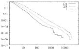
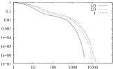
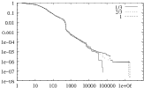
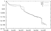
Figure 9: Cumulative degree distributions for different sample sizes ($\frac{1}{3}$ and $\frac{2}{3}$ of the total, and the total itself). From left to right and top to bottom: inet, p2p, web and ip graphs.

One may however observe that for inet and ip the distributions significantly change as the samples grow. In the inet  case one may even be tempted to say that the slope, and thus the exponent of the power-law fit, evolves. We will however avoid such conclusions here: the difference is not significant enough to be observed this way.

In the case of web, only the maximal degree significantly changes. Notice that, in this case, the average degree is roughly constant, meaning that this change in the maximal degree has little impact on the average. This is due to the fact that it concerns only very few nodes. In the case of ip, the changes are mostly between the values $10$ and $200$ of the degree; below and above this interval, the distribution is very stable, and even there the global shape changes only a little.

At this point, it is important to notice that the fact that the degree distributions evolve (for inet and p2p) is not surprising, since the average degree itself evolves, see Section 4.2. In order to deepen this, we need a way to quantify the difference between degree distributions, so that we may observe their evolution more precisely.

The most efficient way to do so probably is to use the classical Kolmogorov-Smirnof (K-S) statistical test, or a similar one. Given two distributions $p_{k}$ and $p^{\prime}_{k}$ which we want to compare, it consists in computing the maximal difference $\max_{k}(|q_{k}-q^{\prime}_{k}|)$ between their respective cumulative distributions $q_{k}$ and $q^{\prime}_{k}$. This test is known to be especially well suited to compare heterogeneous distributions, when one wants to keep the comparison simple.

We display in Figure 10 the values obtained by the K-S test when one compares the degree distribution at each step of the measurement to the final one. This makes it possible to see how the degree distribution evolves towards the final one as the sample size grows.

The K-S test may first have a phase where it varies much but finally reach a phase where its value oscillates close to $0$ (note that it cannot be negative), indicating that the measurement reached a stable view of the degree distribution. This is what we observe in the web and ip cases, confirming the fact that the degree distribution is very stable in these cases (Figure 9). However, the K-S test has a totally different behavior in the other cases: it shows that the degree distribution continuously varies during the measurement. This means that its observation on a particular sample cannot be considered as representative in these cases. We will discuss this further in Section 5.

Figure 10: Evolution of the degree distribution according to a K-S test with the final one, as a function of the sample size. From left to right and top to bottom: inet, p2p, web and ip graphs.

Going further, notice that, in several cases, the evolution of the K-S test is strongly related to the one of the average degree, see Figures 4 and 10: the plots are almost symmetrical for inet and web, and in the two other cases there also seems to be a strong relation between the two statistics. However, there exist cases where their behaviors are very different, which may be observed here for instance for small sizes of the ip samples. This confirms that the K-S test captures other information than simply the average degree, and therefore the similarities observed here are nontrivial: here, the evolution of the degree distributions is well captured by the evolution of the average degree itself, as long as the sample is large enough. In other words, when the average degree does not change, the KS-test (and thus the main properties of the degree distribution) also is stable, in our cases.

Let us finally notice that methods exist to automatically compute the best power-law fit of a distribution according to various criteria. The simplest one probably is a least-square linear fit of the log-log plot, but it can be improved in several ways and more subtle methods exist, see for instance [27, 43]. Such automatic approaches are appealing in our context since they would allow us to plot the evolution of the exponent of the best fit as a function of the sample size.

We tried several such methods, but it appears that our degree distributions are too far from perfect power-laws to give significant results. We tried both with the classical distributions and the cumulative ones, and both with the entire distributions and with parts of them more likely to be well fitted by power-laws. The results remain poor, and vary depending on the used approach (including the fitting method). We therefore consider them as not significant, and we do not present them here.

4.5 Clustering and transitivity.

Despite having a small density, a graph may have a high local density: if two nodes are close to each other in the graph, they are linked together with a much higher probability than two randomly chosen nodes. There is a variety of ways to capture this, the most widely used being to compute the clustering coefficient and/or the transitivity ratio, which we will study in this section.

The clustering coefficient of a node $v$ (of degree at least $2$) is the probability for any two neighbors of $v$ to be linked together: $\mbox{cc}(v)=\frac{2\cdot|E_{N(v)}|}{d^{o}(v)\cdot(d^{o}(v)-1)}$ where $E_{N(v)}=E\cap(N(v)\times N(v))$ is the set of links between neighbors of $v$. Notice that it is nothing but the density of the neighborhood of $v$, and in this sense it captures the local density. The clustering coefficient of the graph itself is the average of this value for all the nodes (of degree at least $2$): $\mbox{cc}=\frac{1}{|\{v\in V,\ d^{o}(v)\geq 2\}|}\sum_{v\in V,\ d^{o}(v)\geq 2}\mbox{cc}(v)$.

One may also define the transitivity ratio of the graph as follows: $\mbox{tr}=\frac{3\cdot N_{\Delta}}{N_{\vee}}$ where $N_{\Delta}$ denotes the number of triangles, i.e. sets of three nodes with three links, in the graph and $N_{\vee}$ denotes the number of connected triples, i.e. sets of three nodes with two links, in the graph.

Computing the clustering coefficient and transitivity ratio is strongly related to counting and/or listing all the triangles in a graph. These problems have been well studied, see [38] for a survey. The fastest known algorithms have a space complexity in $\Theta(n^{2})$, which is prohibitive in our context. Instead, one generally uses a simple algorithm that computes the number of triangles to which each link belongs in $\Theta(n\cdot m)$ time and $\Theta(1)$ space. This is too slow for our purpose, but more subtle algorithms exist with $\Theta(m^{\frac{3}{2}})$ time and $\Theta(n)$ space costs in addition to the $\Theta(m)$ space needed to store the graph. Some of them moreover have the advantage of performing better on graphs with heterogeneous degree distributions like the ones we consider here, see Section 4.4. We use here such an algorithm, namely compact-forward, presented in [47, 38].

4.5.1 Usual assumptions and results.

Concerning clustering coefficients, there are several assumptions commonly accepted as valid. The key ones are the fact that the clustering coefficient and the transitivity ratio are significantly (several orders of magnitude) larger than the density, and that they are independent of the sample size, as long as it is large enough. Moreover, the two notions are generally thought as equivalent.

Figure 11: The clustering coefficient and transitivity ratio as a function of the sample size. From left to right and top to bottom: inet, p2p, web and ip graphs.

Let us first notice that, because of its definition (see Section 3) the ip graph can contain only very few triangles: most of its links are between nodes inside the laboratory and nodes in the outside internet, which prevents triangle formation. Observing the clustering coefficient and the transitivity ratio on such graphs makes little sense. Therefore, we will show the plots but we will not discuss them for this case.

It appears clearly in Figure 11 that the values of both statistics are indeed much larger than the density in our examples (except for ip, as explained above). But it also appears that their value is quite unstable (except in part for p2p); for instance the transitivity ratio in the inet graph experiences a variation of approximately $4$ times its own value. Moreover, the clustering coefficient and the transitivity ratio evolve quite differently (they even have opposite slopes in the web case). Finally, there is no general behavior, except that the observed value is unstable in most cases. This indicates that it is unlikely that one may infer the clustering coefficient or the transitivity ratio of the underlying complex network from such measurements, and that the values obtained on a given sample are not representative (except the transitivity ratio of p2p, in our cases). We will discuss this further in Section 5.

At this point, it is important to notice that for the statistics we observed previously, each one of our graphs conformed to either all or none of the usual assumptions. This is not the case anymore when we take the clustering coefficient and the transitivity ratio into account. Typically, despite the fact that it conforms to all other classical assumptions on the properties we studied until now, web does not have stable values for these new statistics. Conversely, the transitivity ratio of p2p is very stable whereas its observed properties did not match usual assumptions until now. This shows that, while the properties studied in previous sections seem to be strongly related to the average degree, the ones observed here are not.

Figure 12: Maximal degree as a function of the sample size. From left to right and top to bottom: inet, p2p, web and ip graphs.

Figure 13: Number of triangles divided by the square of the maximal degree, as a function of the sample size. From left to right and top to bottom: inet, p2p, web and ip graphs.

One may therefore investigate other explanations. We already observed in Section 4.4 that, in the case of web, the maximal degree is not directly related to the average degree: it varies significantly though the global distribution and the average degree are stable. Going further, we plot the maximal degree $d_{\max}$ of our samples as a function of their size in Figure 12. It seems that it is correlated to the variations of the transitivity ratio. This is due to the fact that the maximal degree node plays a key role in the number of connected triples in the graph: it induces approximately ${d_{\max}}^{2}$ such triples. Therefore, any strong increase of the maximal degree induces a decrease of the transitivity ratio, and when the maximal degree remains stable the transitivity ratio tends to grow or to stay stable . This is confirmed by the plot of the number of triangles divided by the square of the maximal degree, as a function of the sample size, Figure 13, which has a shape similar to the transitivity plots.

Figure 14: Clustering coefficient divided by the density, as a function of the sample size. From left to right and top to bottom: inet, p2p, web and ip graphs.

Concerning the clustering coefficient, which captures the local density, the important points in usual assumptions are that it is several orders of magnitude larger than the (global) density and that it is independent of the sample size. Since the second part of this claim is false, and since the usual assumptions on density are also false, one may wonder how the ratio between the two values evolves. Figure 14 shows that this ratio tends to be constant when the sample becomes very large, especially for the p2p and ip cases. This is a striking observation indicating that the ratio between density and clustering coefficient may be a much more relevant statistical property than the clustering coefficient in our context: it would make sense to seek accurate estimations of this ratio using practical measurements, rather than estimations of the two involved statistics on their own.

5 Conclusion and discussion.

In this paper, we propose the first practical method to rigorously evaluate the relevance of properties observed on large scale complex network measurements. It consists in studying how these properties evolve when the sample grows during the measurement. Complementary to other contributions to this field [35, 10, 6, 28, 20], this method deals directly with real-world data, which has the key advantage of leading to practical results.

We applied this methodology to very large measurements of four different kinds of complex networks. These data-sets are significantly larger than the ones commonly used, and they are representative of the wide variety of complex networks studied in computer science. The classical approach for studying these networks is to collect as much data as possible (which is limited by computing capabilities and measurement time, at least), and then to assume that the obtained sample is representative of the whole.

Our key result is that our methodolody makes it possible to rigorously identify cases where this approach is misleading, whereas in other cases it makes sense and may lead to accurate estimations.

In the case of inet, for instance, the average degree of the sample grows with its size (once it is large enough), which shows clearly that the average degree observed on a particular sample is certainly not the one of the whole graph. In the case of web, on the contrary, the average degree reaches a stable value, indicating that collecting more data probably would not change it. Despite this, the transitivity ratio of this graph is still unstable by the end of the measurement, which shows that a given measurement may reach a stable regime for some of its basic properties while others are still unstable. This is confirmed by p2p, which has a stable transitivity ratio but unstable average degree. These last observations also show that there is no clear hierarchy between properties: the stability or unstability of some properties are independent of each other.

Some observations we made on these examples are in sharp contrast with usual assumptions, thus proving that these assumptions are erroneous in these cases. Other observations are in accordance with them, which provides for the first time a rigorous empirical argument for the relevance of these assumptions in some cases.

More generally, the proposed method makes it possible to distinguish between the two following cases:

• either the property of interest does not reach a stable regime during the measurement, and then this property observed on a given sample certainly is erroneous;

• or the property does reach a stable regime, and then we may conclude that it will probably not evolve anymore and that it is indeed a property of the whole network (though it is possibly biased, see below).

The fact that, even if it is stable, the observed property may be biased is worth deepening. Indeed, it may actually evolve again when the sample grows further (like the average degree in our inet measurement for instance, see Figure 4). This makes the collection of very large data-sets a key issue for our methodology.

This does not entirely solve the problem, however: the property may remain stable until the sample spans almost all the network under concern, but still be significantly biased; finite-size effects may lead to variations in the observation at the end of the measurement (like at its beginning). Moreover, the fact that the underlying network evolves during the measurement should not be neglected anymore. Going even further, one may notice that some measurement techniques are unable to provide a complete view of the network under concern, however how long the measurement is continued (for instance, some links may be invisible from the sources used in a traceroute-based measurement).

Estimating such biases currently is a challenging area of research in which some significant contributions have been made [35, 10, 6, 28, 20], but most remains to be done. The ultimate goal in this direction is to be able to accurately evaluate the actual properties of a complex network from the observation of a (biased) measurement. In the absence of such results, researchers have no choice but to rely on the assumption that the properties they observe do not suffer from such a bias; our method makes it possible to distinguish between cases where this assumption is reasonable, and cases where it must be discarded.

Finally, two other observations obtained in this contribution are worth pointing out.

First, it must be clear that the observed qualitative properties are reliable: they do not depend on the sample size, as long as it is not trivially small. In particular, the average degree is small, the density is close to $0$, the diameter and average distance are small, the degree distributions are heterogeneous, and the clustering coefficient and transitivity ratio are significantly larger than the density (except for ip, as explained in Section 4.5). This is in full accordance with classical qualitative assumptions.

However, as discussed in Section 1, obtaining accurate estimations of the values of the properties is crucial for modeling and simulation: these values are used as key parameters in these contexts and have significant impact on the obtained results. Knowing the qualitative behavior of these properties therefore is unsufficient, and our method constitutes a significant step towards rigorously evaluating their actual values.

Secondly, we gave strong evidence of the fact that the evolution of many subtle statistics is well captured by the evolution of much more basic statistics: the average degree seems to control the general behavior of the average distance and diameter, as well as the evolution of the degree distribution, and the transitivity ratio evolution seems to be governed by the ones of the maximal degree and density. The more complex statistics are not totally controlled by simpler ones, however, and investigating the difference between their behavior and what can be expected would certainly yield enlightening insights. In this spirit, we have shown that the ratio between the clustering coefficient and the density seems significantly more stable than these two statistics on their own.

These observations have to be deepened, but they indicate that the set of relevant statistics for the study of complex networks might be different from what is usually thought: some statistics may be redundant, and other statistics may be more relevant than classical ones (in particular, concerning their accurate evaluation). This raises promising directions for further investigation, in both the analysis and modeling areas.

Acknowledgments. We thank all the colleagues who provided data to us, in particular Paolo Boldi from WebGraph [5], and the people at MetroSec [4], Skitter [1] and Lugdunum [3]. No such work would be possible without their help. We also thank Nicolas Larrieu for great help in managing the data, and Frédéric Aidouni and Fabien Viger for helpful comments and references.
This work was partly funded by the MetroSec (Metrology of the Internet for Security) [4], and the AGRI (Analyse des Grands Réseaux d’Interactions) projects.

References

- [1] Caida – skitter project. http://www.caida.org/tools/measurement/skitter/.
- [2] Data and program – authors’ web page. Removed for anonymous version.
- [3] Lugdunum software. http://lugdunum2k.free.fr/.
- [4] Metrosec project. http://www2.laas.fr/METROSEC/.
- [5] Webgraph project. http://webgraph.dsi.unimi.it/.
- [6] D. Achlioptas, A. Clauset, D. Kempe, and C. Moore. On the bias of traceroute sampling. In ACM STOC, 2005.
- [7] R. Albert, H. Jeong, and A.-L. Barabasi. Diameter of the world wide web. Nature, 401, 1999.
- [8] R. Albert, H. Jeong, and A.-L. Barabási. Error and attack tolerance in complex networks. Nature, 406, 2000.
- [9] N. Alon, Z. Galil, O. Margalit, and M. Naor. Witnesses for boolean matrix multiplication and for shortest paths. In IEEE FOCS, 1992.
- [10] P. Barford, A. Bestavros, J. Byers, and M. Crovella. On the marginal utility of network topology measurements. In ACM/SIGCOMM IMC, 2001.
- [11] P. Boldi and S. Vigna. The webgraph framework i: compression techniques. In WWW, 2004.
- [12] P. Boldi and S. Vigna. The webgraph framework ii: Codes for the world-wide web. In DCC, 2004.
- [13] B. Bollobas. Random Graphs. Cambridge University Press, 2001.
- [14] S. Bornholdt and H.G. Schuster, editors. Hankbook of Graphs and Networks: From the Genome to the Internet. Wiley-VCH, 2003.
- [15] U. Brandes and T. Erlebach, editors. Network Analysis: Methodological Foundations. LNCS, Springer-Verlag, 2005.
- [16] A.Z. Broder, S.R. Kumar, F. Maghoul, P. Raghavan, S. Rajagopalan, R. Stata, A. Tomkins, and J. L. Wiener. Graph structure in the web. Computer Networks, 33, 2000.
- [17] D. Corneil, F. Dragan, M. Habib, and C. Paul. Diameter determination on restricted graph families. Discrete Applied Mathematics, 113(2-3), 2001.
- [18] D.G. Corneil, F.F. Dragan, and E. K hler. On the power of bfs to determine a graph’s diameter. Networks, 42 (4), 2003.
- [19] J.-J. Pansiot D. Magoni. Analysis of the autonomous system network topology. ACM/SIGCOMM Computer Communication Review, 31(3), 2001.
- [20] L. Dall’Asta, J.I. Alvarez-Hamelin, A. Barrat, A. Vazquez, and A. Vespignani. A statistical approach to the traceroute-like exploration of networks: theory and simulations. In CAAN, 2004.
- [21] S.N. Dorogovtsev and J.F.F. Mendes. Handbook of Graphs and Networks: From the Genome to the Internet, chapter Accelerated growth of networks. Wiley-VCH, 2002.
- [22] D. Eppstein and J. Wang. Fast approximation of centrality. Journal of Graph Algorithms and Applications, 8 (1), 2004.
- [23] M. Faloutsos, P. Faloutsos, and C. Faloutsos. On power-law relationships of the internet topology. In ACM SIGCOMM, 1999.
- [24] T. Feder and R. Motwani. Clique partitions, graph compression, and speeding-up algorithms. In ACM STOC, 1991.
- [25] A. Ganesh, L. Massoulie, and D. Towsley. The effect of network topology on the spread of epidemics. In IEEE INFOCOM, 2005.
- [26] C. Gkantsidis, M. Mihail, and E. Zegura. Spectral analysis of internet topologies. In IEEE INFOCOM, 2003.
- [27] Michel L. Goldstein, Steven A. Morris, and Gary G. Yen. Problems with fitting to the power-law distribution. European Physics Journal B, 41, 2004.
- [28] J.-L. Guillaume and M. Latapy. Relevance of massively distributed explorations of the internet topology: Simulation results. In IEEE INFOCOM, 2005.
- [29] J.-L. Guillaume, S. Le-Blond, and M. Latapy. Clustering in p2p exchanges and consequences on performances. In IPTPS, 2005.
- [30] S. Handurukande, A.-M. Kermarrec, F. Le Fessant, and L. Massoulié. Exploiting semantic clustering in the edonkey p2p network. In ACM SIGOPS, 2004.
- [31] H. Jowhari and M. Ghodsi. New streaming algorithms for counting triangles in graphs. In COCOON, 2005.
- [32] M. Kim and M. Medard. Robustness in large-scale random networks. In IEEE INFOCOM, 2004.
- [33] J. M. Kleinberg, R. Kumar, P. Raghavan, S. Rajagopalan, and A. S. Tomkins. The Web as a graph: Measurements, models, and methods. In COCOON, 1999.
- [34] Laas laboratory. http://www.laas.fr/laas/.
- [35] A. Lakhina, J. Byers, M. Crovella, and P. Xie. Sampling biases in ip topology measurements. In IEEE INFOCOM, 2003.
- [36] A. Lakhina, M. Crovella, and C. Diot. Characterization of network-wide anomalies in traffic flows. In ACM/SIGCOMM IMC, 2004.
- [37] A. Lakhina, K. Papagiannaki, M. Crovella, C. Diot, E. Kolaczyk, and N. Taft. Structural analysis of network traffic flows. In ACM/SIGMETRICS Performance, 2004.
- [38] M. Latapy. Theory and practice of triangle problems in very large (sparse (power-law)) graphs. 2006. Submitted.
- [39] S. Le-Blond, M. Latapy, and J.-L. Guillaume. Statistical analysis of a p2p query graph based on degrees and their time evolution. In IWDC, 2004.
- [40] J. Leskovec, J. Kleinberg, and C. Faloutsos. Graphs over time: Densification laws, shrinking diameters and possible explanations. In ACM SIGKDD, 2005.
- [41] Z. Li and P. Mohapatra. Impact of topology on overlay routing service. In IEEE INFOCOM, 2004.
- [42] A. Medina, A. Lakhina, I. Matta, and J. Byers. BRITE: An approach to universal topology generation. In Proc. MASCOTS, 2001. http://www.cs.bu.edu/brite/.
- [43] M.E.J. Newman. Power laws, pareto distributions and zipf’s law. Contemporary Physics, 46:323–351, 2005. cond-mat/0412004.
- [44] M.E.J. Newman, D.J. Watts, and S.H. Strogatz. Random graphs with arbitrary degree distributions and their applications. Phys. Rev. E, 2001.
- [45] C.R. Palmer, P.B. Gibbons, and C. Faloutsos. anf: a fast and scalable tool for data mining in massive graphs. In ACM SIGKDD, 2002.
- [46] R. Pastor-Satorras and A. Vespignani. Epidemic spreading in scale-free networks. Phys. Rev. Let., 86, 2001.
- [47] T. Schank and D. Wagner. Finding, counting and listing all triangles in large graphs, an experimental study. In WEA, 2005.
- [48] Thomas Schank and Dorothea Wagner. Approximating clustering coefficient and transitivity. Journal of Graph Algorithms and Applications (JGAA), 9:2:265–275, 2005.
- [49] R. Seidel. On the all-pairs-shortest-path problem. In ACM STOC, 1992.
- [50] S. Voulgaris, A.-M. Kermarrec, L. Massoulié, and M. van Steen. Exploiting semantic proximity in peer-to-peer content searching. In IEEE FTDCS, 2004.
- [51] D.J. Watts and S.H. Strogatz. Collective dynamics of small-world networks. Nature, 393, 1998.
- [52] U. Zwick. Exact and approximate distances in graphs – A survey. In ESA, volume 2161, 2001.