The Connectivity of Boolean Satisfiability:
Computational and Structural Dichotomies

Abstract

Boolean satisfiability problems are an important benchmark for questions about complexity, algorithms, heuristics and threshold phenomena. Recent work on heuristics, and the satisfiability threshold has centered around the structure and connectivity of the solution space. Motivated by this work, we study structural and connectivity-related properties of the space of solutions of Boolean satisfiability problems and establish various dichotomies in Schaefer’s framework.

On the structural side, we obtain dichotomies for the kinds of subgraphs of the hypercube that can be induced by the solutions of Boolean formulas, as well as for the diameter of the connected components of the solution space. On the computational side, we establish dichotomy theorems for the complexity of the connectivity and $st$-connectivity questions for the graph of solutions of Boolean formulas. Our results assert that the intractable side of the computational dichotomies is PSPACE-complete, while the tractable side - which includes but is not limited to all problems with polynomial time algorithms for satisfiability - is in P for the $st$-connectivity question, and in coNP for the connectivity question. The diameter of components can be exponential for the PSPACE-complete cases, whereas in all other cases it is linear; thus, small diameter and tractability of the connectivity problems are remarkably aligned. The crux of our results is an expressibility theorem showing that in the tractable cases, the subgraphs induced by the solution space possess certain good structural properties, whereas in the intractable cases, the subgraphs can be arbitrary.

1 Introduction

In 1978, T.J. Schaefer [22] introduced a rich framework for expressing variants of Boolean satisfiability and proved a remarkable dichotomy theorem: the satisfiability problem is in P for certain classes of Boolean formulas, while it is NP-complete for all other classes in the framework. In a single stroke, this result pinpoints the computational complexity of all well-known variants of Sat, such as $3$-Sat, Horn 3-Sat, Not-All-Equal $3$-Sat, and $1$-in-$3$ Sat. Schaefer’s work paved the way for a series of investigations establishing dichotomies for several aspects of satisfiability, including optimization [6, 8, 14], counting [7], inverse satisfiability [13], minimal satisfiability [15], $3$-valued satisfiability [5] and propositional abduction [9].

Our aim in this paper is to carry out a comprehensive exploration of a different aspect of Boolean satisfiability, namely, the connectivity properties of the space of solutions of Boolean formulas. The solutions (satisfying assignments) of a given $n$-variable Boolean formula $\varphi$ induce a subgraph $G(\varphi)$ of the $n$-dimensional hypercube. Thus, the following two decision problems, called the connectivity problem and the $st$-connectivity problem, arise naturally: (i) Given a Boolean formula $\varphi$, is $G(\varphi)$ connected? (ii) Given a Boolean formula $\varphi$ and two solutions $\mathbf{s}$ and $\mathbf{t}$ of $\varphi$, is there a path from $\mathbf{s}$ to $\mathbf{t}$ in $G(\varphi)$?

We believe that connectivity properties of Boolean satisfiability merit study in their own right, as they shed light on the structure of the solution space of Boolean formulas. Moreover, in recent years the structure of the space of solutions for random instances has been the main consideration at the basis of both algorithms for and mathematical analysis of the satisfiability problem [2, 21, 20, 18]. It has been conjectured for 3-Sat [20] and proved for 8-Sat [19, 3], that the solution space fractures as one approaches the critical region from below. This apparently leads to performance deterioration of the standard satisfiability algorithms, such as WalkSAT [23] and DPLL [1]. It is also the main consideration behind the design of the survey propagation algorithm, which has far superior performance on random instances of satisfiability [20]. This body of work has served as a motivation to us for pursuing the investigation reported here. While there has been an intensive study of the structure of the solution space of Boolean satisfiability problems for random instances, our work seems to be the first to explore this issue from a worst-case viewpoint.

Our first main result is a dichotomy theorem for the $st$-connectivity problem. This result reveals that the tractable side is much more generous than the tractable side for satisfiability, while the intractable side is PSPACE-complete. Specifically, Schaefer showed that the satisfiability problem is solvable in polynomial time precisely for formulas built from Boolean relations all of which are bijunctive, or all of which are Horn, or all of which are dual Horn, or all of which are affine. We identify new classes of Boolean relations, called tight relations, that properly contain the classes of bijunctive, Horn, dual Horn, and affine relations. We show that $st$-connectivity is solvable in linear time for formulas built from tight relations, and PSPACE-complete in all other cases. Our second main result is a dichotomy theorem for the connectivity problem: it is in coNP for formulas built from tight relations, and PSPACE-complete in all other cases.

In addition to these two complexity-theoretic dichotomies, we establish a structural dichotomy theorem for the diameter of the connected components of the solution space of Boolean formulas. This result asserts that, in the PSPACE-complete cases, the diameter of the connected components can be exponential, but in all other cases it is linear. Thus, small diameter and tractability of the $st$-connectivity problem are remarkably aligned.

To establish these results, the main challenge is to show that for non-tight relations, both the connectivity problem and the $st$-connectivity problem are PSPACE-hard. In Schaefer’s Dichotomy Theorem, NP-hardness of satisfiability was a consequence of an expressibility theorem, which asserted that every Boolean relation can be obtained as a projection over a formula built from clauses in the “hard” relations. Schaefer’s notion of expressibility is inadequate for our problem. Instead, we introduce and work with a delicate and stricter notion of expressibility, which we call faithful expressibility. Intuitively, faithful expressibility means that, in addition to definability via a projection, the space of witnesses of the existential quantifiers in the projection has certain strong connectivity properties that allow us to capture the graph structure of the relation that is being defined. It should be noted that Schaefer’s Dichotomy Theorem can also be proved using a Galois connection and Post’s celebrated classification of the lattice of Boolean clones (see [4]). This method, however, does not appear to apply to connectivity, as the boundaries discovered here cut across Boolean clones. Thus, the use of faithful expressibility or some other refined definability technique seems unavoidable.

The first step towards proving PSPACE-completeness is to show that both connectivity and st-connectivity are hard for 3-CNF formulae; this is proved by a reduction from a generic PSPACE computation. Next, we identify the simplest relations that are not tight: these are ternary relations whose graph is a path of length $4$ between assignments at Hamming distance $2$. We show that these paths can faithfully express all 3-CNF clauses. The crux of our hardness result is an expressibility theorem to the effect that one can faithfully express such a path from any set of relations which is not tight.

Finally, we show that all tight relations have “good” structural properties. Specifically, in a tight relation every component has a unique minimum element, or every component has a unique maximum element, or the Hamming distance coincides with the shortest-path distance in the relation. These properties are inherited by every formula built from tight relations, and yield both small diameter and linear algorithms for $st$-connectivity.

Our original hope was that tractability results for connectivity could conceivably inform heuristic algorithms for satisfiability and enhance their effectiveness. In this context, our findings are prima facie negative: we show that when satisfiability is intractable, then connectivity is also intractable. But our results do contain a glimmer of hope: there are broad classes of intractable satisfiability problems, those built from tight relations, with polynomial $st$-connectivity and small diameter. It would be interesting to investigate if these properties make random instances built from tight relations easier for WalkSAT and similar heuristics, and if so, whether such heuristics are amenable to rigorous analysis.

An extended abstract of this paper appears in ICALP’06 [10].

2 Basic Concepts and Statements of Results

A CNF formula is a Boolean formula of the form $C_{1}\land\dots\land C_{n}$, where each $C_{i}$ is a clause, i.e., a disjunction of literals. If $k$ is a positive integer, then a $k$-CNF formula is a CNF formula $C_{1}\land\dots\land C_{n}$ in which each clause $C_{i}$ is a disjunction of at most $k$ literals.

A logical relation $R$ is a non-empty subset of $\{0,1\}^{k}$, for some $k\geq 1$; $k$ is the arity of $R$. Let ${\cal S}$ be a finite set of logical relations. A CNF$({\cal S})$-formula over a set of variables $V=\{x_{1},\dots,x_{n}\}$ is a finite conjunction $C_{1}\land\dots\land C_{n}$ of clauses built using relations from ${\cal S}$, variables from $V$, and the constants $0$ and $1$; this means that each $C_{i}$ is an expression of the form $R(\xi_{1},\dots,\xi_{k})$, where $R\in{\cal S}$ is a relation of arity $k$, and each $\xi_{j}$ is a variable in $V$ or one of the constants $0$, $1$. A solution of a CNF$({\cal S})$-formula $\varphi$ is an assignment $s=(a_{1},\ldots,a_{n})$ of Boolean values to the variables that makes every clause of $\varphi$ true. A CNF$({\cal S})$-formula is satisfiable if it has at least one solution.

The satisfiability problem Sat$({\cal S})$ associated with a finite set ${\cal S}$ of logical relations asks: given a CNF$({\cal S})$-formula $\varphi$, is it satisfiable? All well known restrictions of Boolean satisfiability, such as $3$-Sat, Not-All-Equal $3$-Sat, and Positive $1$-in-$3$ Sat, can be cast as Sat$({\cal S})$ problems, for a suitable choice of ${\cal S}$. For instance, let $R_{0}=\{0,1\}^{3}\backslash\{000\}$, $R_{1}=\{0,1\}^{3}\backslash\{100\}$, $R_{2}=\{0,1\}^{3}\backslash\{110\}$, $R_{3}=\{0,1\}^{3}\backslash\{111\}$. Then $3$-Sat is the problem Sat$(\{R_{0},R_{1},R_{2},R_{3}\})$. Similarly, Positive 1-in-3Sat is Sat$(\{R_{1/3}\})$, where $R_{1/3}=\{100,010,001\}$.

Schaefer [22] identified the complexity of every satisfiability problem Sat$({\cal S})$, where ${\cal S}$ ranges over all finite sets of logical relations. To state Schaefer’s main result, we need to define some basic concepts.

Definition 1.

Let $R$ be a logical relation.

1. $R$ is bijunctive if it is the set of solutions of a 2-CNF formula.

2. $R$ is Horn if it is the set of solutions of a Horn formula, where a Horn formula is a CNF formula such that each conjunct has at most one positive literal.

3. $R$ is dual Horn if it is the set of solutions of a dual Horn formula, where a dual Horn formula is a CNF formula such that each conjunct has at most one negative literal.

4. $R$ is affine if it is the set of solutions of a system of linear equations over $\mathbb{Z}_{2}$.

Each of these types of logical relations can be characterized in terms of closure properties [22]. A relation $R$ is bijunctive if and only if it is closed under the majority operation; this means that if $\mathbf{a},\mathbf{b},\mathbf{c}\in R$, then $\operatorname{maj}(\mathbf{a},\mathbf{b},\mathbf{c})\in R$, where $\operatorname{maj}(\mathbf{a},\mathbf{b},\mathbf{c})$ is the vector whose $i$-th bit is the majority of $a_{i},b_{i},c_{i}$. A relation $R$ is Horn if and only if it is closed under $\vee$; this means that if $\mathbf{a},\mathbf{b}\in R$, then $\mathbf{a}\vee\mathbf{b}\in R$, where, $\mathbf{a}\vee\mathbf{b}$ is the vector whose $i$-th bit is $a_{i}\vee b_{i}$. Similarly, $R$ is dual Horn if and only if it is closed under $\wedge$. Finally, $R$ is affine if and only if it is closed under $\mathbf{a}\oplus\mathbf{b}\oplus\mathbf{c}$. Thus there is a polynomial-time algorithm (in fact, a cubic algorithm) to test if a relation is Schaefer.

Definition 2.

A set ${\cal S}$ of logical relations is Schaefer if at least one of the following conditions holds:

1. Every relation in ${\cal S}$ is bijunctive.

2. Every relation in ${\cal S}$ is Horn.

3. Every relation in ${\cal S}$ is dual Horn.

4. Every relation in ${\cal S}$ is affine.

Theorem 3.

(Schaefer’s Dichotomy Theorem [22]) Let $\cal S$ be a finite set of logical relations. If ${\cal S}$ is Schaefer, then Sat$({\cal S})$ is in P; otherwise, Sat$({\cal S})$ is NP-complete.

Theorem 3 is called a dichotomy theorem because Ladner [16] has shown that if ${\rm P}\not={\rm NP}$, then there are problems in NP that are neither in P, nor NP-complete. Thus, Theorem 3 asserts that no Sat$({\cal S})$ problem is a problem of the kind discovered by Ladner. Note that the aforementioned characterization of Schaefer sets in terms of closure properties yields a cubic algorithm for determining, given a finite set $\cal S$ of logical relations, whether Sat$({\cal S})$ is in P or is NP-complete (here, the input size is the sum of the sizes of the relations in $\cal S$).

The more difficult part of the proof of Schafer’s Dichotomy Theorem is to show that if $\cal S$ is not Schaefer, then Sat$({\cal S})$ is NP-complete. This is a consequence of a powerful result about the expressibility of logical relations. We say that a relation $R$ is expressible from a set ${\cal S}$ of relations if there is a CNF$({\cal S})$-formula $\varphi({\bf x},{\bf y})$ such that $R=\{{\bf a}|\exists\mathbf{y}~{}\varphi(\mathbf{a},\mathbf{y})\}$.

Theorem 4.

(Schaefer’s Expressibility Theorem [22]) Let $\cal S$ be a finite set of logical relations. If ${\cal S}$ is not Schaefer, then every logical relation is expressible from ${\cal S}$.

In this paper, we are interested in the connectivity properties of the space of solutions of CNF$({\cal S})$-formulas. If $\varphi$ is a CNF$({\cal S})$-formula with $n$ variables, then the solution graph $G(\varphi)$ of $\varphi$ denotes the subgraph of the $n$-dimensional hypercube induced by the solutions of $\varphi$. This means that the vertices of $G(\varphi)$ are the solutions of $\varphi$, and there is an edge between two solutions of $G(\varphi)$ precisely when they differ in exactly one variable.

We consider the following two algorithmic problems for CNF$({\cal S})$-formulas.

Problem 1.

The Connectivity Problem Conn$({\cal S})$:

Given a CNF$({\cal S})$-formula $\varphi$, is $G(\varphi)$ connected?

Problem 2.

The st-Connectivity Problem st-Conn$({\cal S})$:

Given a CNF$({\cal S})$-formula $\varphi$ and two solutions $\mathbf{s}$ and $\mathbf{t}$ of $\varphi$, is there a path from $\mathbf{s}$ to $\mathbf{t}$ in $G(\varphi)$?

To pinpoint the computational complexity of Conn$({\cal S})$ and st-Conn$({\cal S})$, we need to introduce certain new types of relations.

Definition 5.

Let $R\subseteq\{0,1\}^{k}$ be a logical relation.

1. $R$ is componentwise bijunctive if every connected component of the graph $G(R)$ is a bijunctive relation.

2. $R$ is OR-free if the relation ${\rm OR}=\{01,10,11\}$ cannot be obtained from $R$ by setting $k-2$ of the coordinates of $R$ to a constant $\mathbf{c}\in\{0,1\}^{k-2}$. In other words, $R$ is OR-free if $(x_{1}\lor x_{2})$ is not definable from $R$ by fixing $k-2$ variables.

3. $R$ is NAND-free if the relation ${\rm NAND}=\{00,01,10\}$ cannot be obtained from $R$ by setting $k-2$ of the coordinates of $R$ to a constant $\mathbf{c}\in\{0,1\}^{k-2}$. In other words, $R$ is NAND-free is $(\bar{x}_{1}\vee\bar{x}_{2})$ is not definable from $R$ by fixing $k-2$ variables.

We are now ready to introduce the key concept of a tight set of relations.

Definition 6.

A set ${\cal S}$ of logical relations is tight if at least one of the following three conditions holds:

1. Every relation in ${\cal S}$ is componentwise bijunctive;

2. Every relation in ${\cal S}$ is OR-free;

3. Every relation in ${\cal S}$ is NAND-free.

In Section 4, we show that if ${\cal S}$ is Schaefer, then it is tight. Moreover, we show that the converse does not hold. It is also easy to see that there is a polynomial-time algorithm (in fact, a cubic algorithm) for testing whether a given relation is tight.

Just as Schaefer’s dichotomy theorem follows from an expressibility statement, our dichotomy theorems are derived from the following theorem, which we will call the Faithful Expressibility Theorem. The precise definition of the concept of faithful expressibility is given in Section 3. Intuitively, this concept strengthens the concept of expressibility with the requirement that the space of the witnesses to the existentially quantified variables has certain strong connectivity properties.

Theorem 7.

(Faithful Expressibility Theorem) Let $\cal S$ be a finite set of logical relations. If ${\cal S}$ is not tight, then every logical relation is faithfully expressible from ${\cal S}$.

Using the Faithful Expressibility Theorem, we obtain the following dichotomy theorems for the computational complexity of Conn$({\cal S})$ and st-Conn$({\cal S})$.

Theorem 8.

Let ${\cal S}$ be a finite set of logical relations. If ${\cal S}$ is tight, then Conn$({\cal S})$ is in coNP; otherwise, it is PSPACE-complete.

Theorem 9.

Let ${\cal S}$ be a finite set of logical relations. If ${\cal S}$ is tight, then st-Conn$({\cal S})$ is in P; otherwise, st-Conn$({\cal S})$ is PSPACE-complete.

We also show that if ${\cal S}$ is tight, but not Schaefer, then Conn$({\cal S})$ is coNP-complete.

To illustrate these results, consider the set ${\cal S}=\{R_{1/3}\}$, where $R_{1/3}=\{100,010,001\}$. This set is tight (actually, it is componentwise bijunctive), but not Schaefer. It follows that Sat$({\cal S})$ is NP-complete (recall that this problem is Positive 1-in-3 Sat), st-Conn$({\cal S})$ is in P, and Conn$({\cal S})$ is coNP-complete. Consider also the set ${\cal S}=\{R_{\rm{NAE}}\}$, where $R_{\rm{NAE}}=\{0,1\}^{3}\setminus\{000,111\}$. This set is not tight, hence Sat$({\cal S})$ is NP-complete (this problem is Positive Not-All-Equal 3-Sat), while both st-Conn$({\cal S})$ and Conn$({\cal S})$ are PSPACE-complete.

The dichotomy in the computational complexity of Conn$({\cal S})$ and st-Conn$({\cal S})$ is accompanied by a parallel structural dichotomy in the size of the diameter of $G(\varphi)$ (where, for a CNF$({\cal S})$-formula $\varphi$, the diameter of $G(\varphi)$ is the maximum of the diameters of the components of $G(\varphi)$).

Theorem 10.

Let ${\cal S}$ be a finite set of logical relations. If ${\cal S}$ is tight, then for every CNF$({\cal S})$-formula $\varphi$, the diameter of $G(\varphi)$ is linear in the number of variables of $\varphi$; otherwise, there are CNF$({\cal S})$-formulas $\varphi$ such that the diameter of $G(\varphi)$ is exponential in the number of variables of $\varphi$.

Our results and their comparison to Schaefer’s Dichotomy Theorem are summarized in the table below.

${\cal S}$	Sat$({\cal S})$	st-Conn$({\cal S})$	Conn$({\cal S})$	Diameter
Schaefer	P	P	coNP	$O(n)$
Tight, non-Schaefer	NP-compl.	P	coNP-compl.	$O(n)$
Non-tight	NP-compl.	PSPACE-compl.	PSPACE-compl.	$2^{\Omega(\sqrt{n})}$

We conjecture that the complexity of Conn$({\cal S})$ exhibits a trichotomy, that is, for every finite set $\cal S$ of logical relations, one of the following holds:

1. Conn$({\cal S})$ is in P;

2. Conn$({\cal S})$ is coNP-complete;

3. Conn$({\cal S})$ is PSPACE-complete.

As mentioned above, we will show that if ${\cal S}$ is tight but not Schaefer, then Conn$({\cal S})$ is coNP-complete. We will also show that if ${\cal S}$ is bijunctive or affine, then Conn$({\cal S})$ is in P. Hence, to settle the above conjecture, it remains to pinpoint the complexity of Conn$({\cal S})$ whenever $\cal S$ is Horn and whenever $\cal S$ is dual Horn. In the conference version [10] of the present paper, we further conjectured that if ${\cal S}$ is Horn or dual Horn, then Conn$({\cal S})$ is in P. In other words, we conjectured that if ${\cal S}$ is Schaefer, then Conn$({\cal S})$ is in P. This second conjecture, however, was subsequently disproved by Makino, Tanaka and Yamamato [17], who discovered a particular Horn set ${\cal S}$ such that Conn$({\cal S})$ is coNP-complete. Here, we go beyond the results obtained in the conference version of the present paper and identify additional conditions on a Horn set $\cal S$ implying that Conn$({\cal S})$ is in P. These new results suggest a natural dichotomy within Schaefer sets of relations and, thus, provide evidence for the trichotomy conjecture.

The remainder of this paper is organized as follows. In Section 3, we prove the Faithful Expressibility Theorem, establish the hard side of the dichotomies for Conn$({\cal S})$ and for st-Conn$({\cal S})$, and contrast our result to Schaefer’s Expressibility and Dichotomy Theorems. In Section 4, we describe the easy side of the dichotomy - the polynomial-time algorithms and the structural properties for tight sets of relations. In addition, we obtain partial results towards the trichotomy conjecture for Conn$({\cal S})$.

3 The Hard Case of the Dichotomy: Non-Tight Sets of Relations

In this section, we address the hard side of the dichotomy, where we deal with the more computationally intractable cases. As with other dichotomy theorems, this is also the harder part of our proof. We define the notion of faithful expressibility in Section 3.1 and prove the Faithful Expressibility Theorem in Section 3.2. This theorem implies that for all non-tight sets $\cal S$ and ${\cal S^{\prime}}$, the connectivity problems Conn$({\cal S})$ and Conn$({\cal S^{\prime}})$ are polynomial-time equivalent; moreover, the same holds true for the connectivity problems st-Conn$({\cal S})$ and st-Conn$({\cal S^{\prime}})$. In addition, the diameters of the solution graphs of CNF$({\cal S})$-formulas and CNF$({\cal S^{\prime}})$-formulas are also related polynomially. In Section 3.3, we prove that for 3-CNF formulas the connectivity problems are PSPACE-complete, and the diameter can be exponential. This fact combined with the Faithful Expressibility Theorem yields the hard side of all of our dichotomy results, as well as the exponential size of the diameter.

We will use $\mathbf{a},\mathbf{b},\dots$ to denote Boolean vectors, and $\mathbf{x}$ and $\mathbf{y}$ to denote vectors of variables. We write $|\mathbf{a}|$ to denote the Hamming weight (number of $1$’s) of a Boolean vector $\mathbf{a}$. Given two Boolean vectors $\mathbf{a}$ and $\mathbf{b}$, we write $|\mathbf{a}-\mathbf{b}|$ to denote the Hamming distance between $\mathbf{a}$ and $\mathbf{b}$. Finally, if $\mathbf{a}$ and $\mathbf{b}$ are solutions of a Boolean formula $\varphi$ and lie in the same component of $G(\varphi)$, then we write $d_{\varphi}(\mathbf{a},\mathbf{b})$ to denote the shortest-path distance between $\mathbf{a}$ and $\mathbf{b}$ in $G(\varphi)$.

3.1 Faithful Expressibility

As we mentioned in the previous section, in his dichotomy theorem, Schaefer [22] used the following notion of expressibility: a relation $R$ is expressible from a set ${\cal S}$ of relations if there is a CNF$({\cal S})$-formula $\varphi$ so that $R=\{\mathbf{a}|~{}\exists\mathbf{y}~{}\varphi(\mathbf{a},\mathbf{y})\}$. This notion, is not sufficient for our purposes. Instead, we introduce a more delicate notion, which we call faithful expressibility. Intuitively, we view the relation $R$ as a subgraph of the hypercube, rather than just a subset, and require that this graph structure be also captured by the formula $\varphi$.

(a)

(b)                                                        (c)

Fig. 1: Expressing the relation $(x_{1}\vee x_{2}\vee x_{3})$ using Not-All-Equal relations.
(a) Graph of $(x_{1}\vee x_{2}\vee x_{3})$;
(b) Graph of a faithful expression: $\varphi(\mathbf{x},y_{1},y_{2})=R_{\rm{NAE}}(x_{1},x_{2},y_{1})\wedge R_{\rm{NAE}}(x_{2},x_{3},y_{2})\wedge R_{\rm{NAE}}(y_{1},y_{2},1).$
(c) Graph of an unfaithful expression: $\varphi(\mathbf{x},y_{1})=R_{\rm{NAE}}(x_{1},x_{2},y_{1})\wedge R_{\rm{NAE}}(\bar{y}_{1},x_{3},0)\wedge R_{\rm{NAE}}(y_{1},x_{2},1).$
In both cases $(x_{1}\vee x_{2}\vee x_{3})=\exists\mathbf{y}~{}\varphi(\mathbf{x},\mathbf{y})$, but only in the first case the connectivity is preserved.

Definition 11.

A relation $R$ is faithfully expressible from a set of relations ${\cal S}$ if there is a CNF$({\cal S})$-formula $\varphi$ such that the following conditions hold:

1. $R=\{\mathbf{a}|~{}\exists\mathbf{y}~{}\varphi(\mathbf{a},\mathbf{y})\}$;

2. For every $\mathbf{a}\in R$, the graph $G(\varphi(\mathbf{a},\mathbf{y}))$ is connected;

3. For $\mathbf{a},\mathbf{b}\in R$ with $|\mathbf{a}-\mathbf{b}|=1$, there exists $\mathbf{w}$ such that $(\mathbf{a},\mathbf{w})$ and $(\mathbf{b},\mathbf{w})$ are solutions of $\varphi$.

For $\mathbf{a}\in R$, the witnesses of $\mathbf{a}$ are the $\mathbf{y}$’s such that $\varphi(\mathbf{a},\mathbf{y})$ is true. The last two conditions say that the witnesses of $\mathbf{a}\in R$ are connected, and that neighboring $\mathbf{a},\mathbf{b}\in R$ have a common witness. This allows us to simulate an edge $(\mathbf{a},\mathbf{b})$ in $G(R)$ by a path in $G(\varphi)$, and thus relate the connectivity properties of the solution spaces. There is however, a price to pay: it is much harder to come up with formulas that faithfully express a relation $R$. An example is when ${\cal S}$ is the set of all paths of length $4$ in $\{0,1\}^{3}$, a set that plays a crucial role in our proof. While 3-Sat relations are easily expressible from ${\cal S}$ in Schaefer’s sense, the CNF$({\cal S})$-formulas that faithfully express 3-Sat relations are fairly complicated and have a large witness space.

An example of the difference between a faithful and an unfaithful expression is shown in Figure 1.

Lemma 12.

Let ${\cal S}$ and ${\cal S}^{\prime}$ be sets of relations such that every $R\in{\cal S}^{\prime}$ is faithfully expressible from ${\cal S}$. Given a CNF$({\cal S}^{\prime})$-formula $\psi(\mathbf{x})$, one can efficiently construct a CNF$({\cal S})$-formula $\varphi(\mathbf{x},\mathbf{y})$ such that:

1. $\psi(\mathbf{x})\equiv\exists\mathbf{y}~{}\varphi(\mathbf{x},\mathbf{y})$;

2. if $(\mathbf{s},\mathbf{w^{s}}),(\mathbf{t},\mathbf{w^{t}})\in\varphi$ are connected in $G(\varphi)$ by a path of length $d$, then there is a path from $\mathbf{s}$ to $\mathbf{t}$ in $G(\psi)$ of length at most $d$;

3. If $\mathbf{s},\mathbf{t}\in\psi$ are connected in $G(\psi)$, then for every witness $\mathbf{w^{s}}$ of $\mathbf{s}$, and every witness $\mathbf{w^{t}}$ of $\mathbf{t}$, there is a path from $(\mathbf{s},\mathbf{w^{s}})$ to $(\mathbf{t},\mathbf{w^{t}})$ in $G(\varphi)$.

Proof.

Suppose $\psi$ is a formula on $n$ variables that consists of $m$ clauses $C_{1},\dots,C_{m}$. For clause $C_{j}$, assume that the set of variables is $V_{j}\subseteq[n]$, and that it involves relation $R_{j}\in{\cal S}$. Thus, $\psi(\mathbf{x})$ is $\wedge_{j=1}^{m}R_{j}(\mathbf{x}_{V_{j}})$. Let $\varphi_{j}$ be the faithful expression for $R_{j}$ from ${\cal S}^{\prime}$, so that $R_{j}(\mathbf{x}_{V_{j}})\equiv\exists\mathbf{y}_{j}~{}\varphi_{j}(\mathbf{x}_{V_{j}},\mathbf{y}_{j})$. Let $\mathbf{y}$ be the vector $(\mathbf{y}_{1},\dots,\mathbf{y}_{m})$ and let $\varphi(\mathbf{x},\mathbf{y})$ be the formula $\wedge_{j=1}^{m}\varphi_{j}(\mathbf{x}_{V_{j}},\mathbf{y}_{j})$. Then $\psi(\mathbf{x})\equiv\exists\mathbf{y}~{}\varphi(\mathbf{x},\mathbf{y})$.

Statement $(2)$ follows from $(1)$ by projection of the path on the coordinates of $\mathbf{x}$. For statement $(3)$, consider $\mathbf{s},\mathbf{t}\in\psi$ that are connected in $G(\psi)$ via a path $\mathbf{s}=\mathbf{u^{0}}\rightarrow\mathbf{u^{1}}\rightarrow\dots\rightarrow\mathbf{u^{r}}=\mathbf{t}$ . For every $\mathbf{u^{i}},\mathbf{u^{i+1}}$, and clause $C_{j}$, there exists an assignment $\mathbf{w^{i}}_{j}$ to $\mathbf{y}_{j}$ such that both $(\mathbf{u^{i}}_{V_{j}},\mathbf{w^{i}}_{j})$ and $(\mathbf{u^{i+1}}_{V_{j}},\mathbf{w^{i}}_{j})$ are solutions of $\varphi_{j}$, by condition $(2)$ of faithful expressibility. Thus $(\mathbf{u^{i}},\mathbf{w^{i}})$ and $(\mathbf{u^{i+1}},\mathbf{w^{i}})$ are both solutions of $\varphi$, where $\mathbf{w^{i}}=(\mathbf{w^{i}}_{1},\dots\mathbf{w^{i}}_{m})$. Further, for every $\mathbf{u^{i}}$, the space of solutions of $\varphi(\mathbf{u^{i}},\mathbf{y})$ is the product space of the solutions of $\varphi_{j}(\mathbf{u^{i}}_{V_{j}},\mathbf{y}_{j})$ over $j=1,\dots,m$. Since these are all connected by condition $(3)$ of faithful expressibility, $G(\varphi(\mathbf{u^{i}},\mathbf{y}))$ is connected. The following describes a path from $(\mathbf{s},\mathbf{w^{s}})$ to $(\mathbf{t},\mathbf{w^{t}})$ in $G(\varphi)$:  $(\mathbf{s},\mathbf{w^{s}})\rightsquigarrow(\mathbf{s},\mathbf{w^{0}})\rightarrow(\mathbf{u^{1}},\mathbf{w^{0}})\rightsquigarrow(\mathbf{u^{1}},\mathbf{w^{1}})\rightarrow\dots\rightsquigarrow(\mathbf{u^{r-1}},\mathbf{w^{r-1}})\rightarrow(\mathbf{t},\mathbf{w^{r-1}})\rightsquigarrow(\mathbf{t},\mathbf{w^{t}})$. Here $\rightsquigarrow$ indicates a path in $G(\varphi(\mathbf{u^{i}},\mathbf{y}))$. ∎

Corollary 13.

Suppose ${\cal S}$ and ${\cal S}^{\prime}$ are sets of relations such that every $R\in{\cal S}^{\prime}$ is faithfully expressible from ${\cal S}$.

1. There are polynomial time reductions from Conn$({\cal S^{\prime}})$ to Conn$({\cal S})$, and from st-Conn$({\cal S^{\prime}})$ to st-Conn$({\cal S})$.

2. Given a CNF$({\cal S^{\prime}})$-formula $\psi(\mathbf{x})$ with $m$ clauses, one can efficiently construct a CNF$({\cal S})$-formula $\varphi(\mathbf{x},\mathbf{y})$ such that the length of $\mathbf{y}$ is $O(m)$ and the diameter of the solution space does not decrease.

3.2 The Faithful Expressibility Theorem

In this subsection, we prove the Faithful Expressibility Theorem. The main step in the proof is Lemma 14 which shows that if ${\cal S}$ is not tight, then we can faithfully express the 3-clause relations from the relations in ${\cal S}$. If $k\geq 2$, then a $k$-clause is a disjunction of $k$ variables or negated variables. For $0\leq i\leq k$, let $D_{i}$ be the set of all satisfying truth assignments of the $k$-clause whose first $i$ literals are negated, and let ${\cal S}_{k}=\{D_{0},D_{1},\dots,D_{k}\}$. Thus, CNF$({\cal S}_{k})$ is the collection of $k$-CNF formulas.

Lemma 14.

If set ${\cal S}$ of relations is not tight, ${\cal S}_{3}$ is faithfully expressible from ${\cal S}$.

Proof.

First, observe that all $2$-clauses are faithfully expressible from ${\cal S}$. There exists $R\in{\cal S}$ which is not OR-free, so we can express $(x_{1}\vee x_{2})$ by substituting constants in $R$. Similarly, we can express $(\bar{x}_{1}\vee\bar{x}_{2})$ using a relation that is not NAND-free. The last 2-clause $(x_{1}\vee\bar{x}_{2})$ can be obtained from OR and NAND by a technique that corresponds to reverse resolution. $(x_{1}\vee\bar{x}_{2})=\exists y~{}(x_{1}\vee y)\wedge(\bar{y}\vee\bar{x}_{2})$. It is easy to see that this gives a faithful expression. From here onwards we assume that ${\cal S}$ contains all 2-clauses. The proof now proceeds in four steps. First, we will express a relation in which there exist two elements that are at graph distance larger than their Hamming distance. Second, we will express a relation that is just a single path between such elements. Third, we will express a relation which is a path of length 4 between elements at Hamming distance 2. Finally, we will express the 3-clauses.

Step 1.

Faithfully expressing a relation in which some distance expands.

For a relation $R$, we say that the distance between $\mathbf{a}$ and $\mathbf{b}$ expands if $\mathbf{a}$ and $\mathbf{b}$ are connected in $G(R)$, but $d_{R}(\mathbf{a},\mathbf{b})>|\mathbf{a}-\mathbf{b}|$. Later on, we will show that no distance expands in componentwise bijunctive relations. The same also holds true for the relation $R_{\rm{NAE}}=\{0,1\}^{3}\setminus\{000,111\}$, which is not componentwise bijunctive. Nonetheless, we show here that if $R$ is not componentwise bijunctive, then, by adding $2$-clauses, we can faithfully express a relation $Q$ in which some distance expands. For instance, when $R=R_{\rm NAE}$, then we can take $Q(x_{1},x_{2},x_{3})=R_{\rm NAE}(x_{1},x_{2},x_{3})\wedge(\bar{x_{1}}\vee\bar{x}_{3})$. The distance between $\mathbf{a}=100$ and $\mathbf{b}=001$ in $Q$ expands. Similarly, in the general construction, we identify $\mathbf{a}$ and $\mathbf{b}$ on a cycle, and add $2$-clauses that eliminate all the vertices along the shorter arc between $\mathbf{a}$ and $\mathbf{b}$.

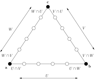
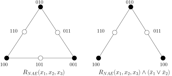
Fig. 2: Proof of Step 1 of Lemma 14, and an example.

Since ${\cal S}$ is not tight, it contains a relation $R$ which is not componentwise bijunctive. If $R$ contains $\mathbf{a},\mathbf{b}$ where the distance between them expands, we are done. So assume that for all $\mathbf{a},\mathbf{b}\in G(R)$, $d_{R}(\mathbf{a},\mathbf{b})=|\mathbf{a}-\mathbf{b}|$. Since $R$ is not componentwise bijunctive, there exists a triple of assignments $\mathbf{a},\mathbf{b},\mathbf{c}$ lying in the same component such that $\operatorname{maj}(\mathbf{a},\mathbf{b},\mathbf{c})$ is not in that component (which also easily implies it is not in $R$). Choose the triple such that the sum of pairwise distances $d_{R}(\mathbf{a},\mathbf{b})+d_{R}(\mathbf{b},\mathbf{c})+d_{R}(\mathbf{c},\mathbf{a})$ is minimized. Let $U=\{i|a_{i}\neq b_{i}\}$, $V=\{i|b_{i}\neq c_{i}\}$, and $W=\{i|c_{i}\neq a_{i}\}$. Since $d_{R}(\mathbf{a},\mathbf{b})=|\mathbf{a}-\mathbf{b}|$, a shortest path does not flip variables outside of $U$, and each variable in $U$ is flipped exactly once. The same holds for $V$ and $W$. We note some useful properties of the sets $U,V,W$.

1. Every index $i\in U\cup V\cup W$ occurs in exactly two of $U,V,W$.
   Consider going by a shortest path from $\mathbf{a}$ to $\mathbf{b}$ to $\mathbf{c}$ and back to $\mathbf{a}$. Every $i\in U\cup V\cup W$ is seen an even number of times along this path since we return to $\mathbf{a}$. It is seen at least once, and at most thrice, so in fact it occurs twice.

2. Every pairwise intersection $U\cap V,V\cap W$ and $W\cap U$ is non-empty.
   Suppose the sets $U$ and $V$ are disjoint. From Property 1, we must have $W=U\cup V$. But then it is easy to see that $\operatorname{maj}(\mathbf{a},\mathbf{b},\mathbf{c})=\mathbf{b}$ which is in $R$. This contradicts the choice of $\mathbf{a},\mathbf{b},\mathbf{c}$.

3. The sets $U\cap V$ and $U\cap W$ partition the set $U$.
   By Property $1$, each index of $U$ occurs in one of $V$ and $W$ as well. Also since no index occurs in all three sets $U,V,W$ this is in fact a disjoint partition.

4. For each index $i\in U\cap W$, it holds that $\mathbf{a}\oplus\mathbf{e}_{i}\not\in R$.
   Assume for the sake of contradiction that $\mathbf{a^{\prime}}=\mathbf{a}\oplus\mathbf{e}_{i}\in R$. Since $i\in U\cap W$ we have simultaneously moved closer to both $\mathbf{b}$ and $\mathbf{c}$. Hence we have $d_{R}(\mathbf{a^{\prime}},\mathbf{b})+d_{R}(\mathbf{b},\mathbf{c})+d_{R}(\mathbf{c},\mathbf{a^{\prime}})<d_{R}(\mathbf{a},\mathbf{b})+d_{R}(\mathbf{b},\mathbf{c})+d_{R}(\mathbf{c},\mathbf{a})$. Also $\operatorname{maj}(\mathbf{a^{\prime}},\mathbf{b},\mathbf{c})=\operatorname{maj}(\mathbf{a},\mathbf{b},\mathbf{c})\not\in R$. But this contradicts our choice of $\mathbf{a},\mathbf{b},\mathbf{c}$.

Property 4 implies that the shortest paths to $\mathbf{b}$ and $\mathbf{c}$ diverge at $\mathbf{a}$, since for any shortest path to $\mathbf{b}$ the first variable flipped is from $U\cap V$ whereas for a shortest path to $\mathbf{c}$ it is from $W\cap V$. Similar statements hold for the vertices $\mathbf{b}$ and $\mathbf{c}$. Thus along the shortest path from $\mathbf{a}$ to $\mathbf{b}$ the first bit flipped is from $U\cap V$ and the last bit flipped is from $U\cap W$. On the other hand, if we go from $\mathbf{a}$ to $\mathbf{c}$ and then to $\mathbf{b}$, all the bits from $U\cap W$ are flipped before the bits from $U\cap V$. We use this crucially to define $Q$. We will add a set of 2-clauses that enforce the following rule on paths starting at $\mathbf{a}$: Flip variables from $U\cap W$ before variables from $U\cap V$. This will eliminate all shortest paths from $\mathbf{a}$ to $\mathbf{b}$ since they begin by flipping a variable in $U\cap V$ and end with $U\cap W$. The paths from $\mathbf{a}$ to $\mathbf{b}$ via $\mathbf{c}$ survive since they flip $U\cap W$ while going from $\mathbf{a}$ to $\mathbf{c}$ and $U\cap V$ while going from $\mathbf{c}$ to $\mathbf{b}$. However all remaining paths have length at least $|\mathbf{a}-\mathbf{b}|+2$ since they flip twice some variables not in $U$.

Take all pairs of indices $\{(i,j)|i\in U\cap W,j\in U\cap V\}$. The following conditions hold from the definition of $U,V,W$: $a_{i}=\bar{c}_{i}=\bar{b}_{i}$ and $a_{j}=c_{j}=\bar{b}_{j}$. Add the 2-clause $C_{ij}$ asserting that the pair of variables $x_{i}x_{j}$ must take values in $\{a_{i}a_{j},c_{i}c_{j},b_{i}b_{j}\}=\{a_{i}a_{j},\bar{a}_{i}a_{j},\bar{a}_{i}\bar{a}_{j}\}$. The new relation is $Q=R\wedge_{i,j}C_{ij}$. Note that $Q\subset R$. We verify that the distance between $\mathbf{a}$ and $\mathbf{b}$ in $Q$ expands. It is easy to see that for any $j\in U$, the assignment $\mathbf{a}\oplus\mathbf{e}_{j}\not\in Q$. Hence there are no shortest paths left from $\mathbf{a}$ to $\mathbf{b}$. On the other hand, it is easy to see that $\mathbf{a}$ and $\mathbf{b}$ are still connected, since the vertex $\mathbf{c}$ is still reachable from both.

Step 2.

Isolating a pair of assignments whose distance expands.

The relation $Q$ obtained in Step 1 may have several disconnected components. This cleanup step isolates a single pair of assignments whose distance expands. By adding $2$-clauses, we show that one can express a path of length $r+2$ between assignments at distance $r$.

Take $\mathbf{a},\mathbf{b}\in Q$ whose distance expands in $Q$ and $d_{Q}(\mathbf{a},\mathbf{b})$ is minimized. Let $U=\{i|a_{i}\neq b_{i}\}$, and $|U|=r$. Shortest paths between $\mathbf{a}$ and $\mathbf{b}$ have certain useful properties:

1. Each shortest path flips every variable from $U$ exactly once.
   Observe that each index $j\in U$ is flipped an odd number of times along any path from $\mathbf{a}$ to $\mathbf{b}$. Suppose it is flipped thrice along a shortest path. Starting at $\mathbf{a}$ and going along this path, let $\mathbf{b^{\prime}}$ be the assignment reached after flipping $j$ twice. Then the distance between $\mathbf{a}$ and $\mathbf{b^{\prime}}$ expands, since $j$ is flipped twice along a shortest path between them in $Q$. Also $d_{Q}(\mathbf{a},\mathbf{b^{\prime}})<d_{Q}(\mathbf{a},\mathbf{b})$, contradicting the choice of $\mathbf{a}$ and $\mathbf{b}$.

2. Every shortest path flips exactly one variable $i\not\in U$.
   Since the distance between $\mathbf{a}$ and $\mathbf{b}$ expands, every shortest path must flip some variable $i\not\in U$. Suppose it flips more than one such variable. Since $\mathbf{a}$ and $\mathbf{b}$ agree on these variables, each of them is flipped an even number of times. Let $i$ be the first variable to be flipped twice. Let $\mathbf{b^{\prime}}$ be the assignment reached after flipping $i$ the second time. It is easy to verify that the distance between $\mathbf{a}$ and $\mathbf{b^{\prime}}$ also expands, but $d_{Q}(\mathbf{a},\mathbf{b^{\prime}})<d_{Q}(\mathbf{a},\mathbf{b})$.

3. The variable $i\not\in U$ is the first and last variable to be flipped along the path. Assume the first variable flipped is not $i$. Let $\mathbf{a^{\prime}}$ be the assignment reached along the path before we flip $i$ the first time. Then $d_{Q}(\mathbf{a^{\prime}},\mathbf{b})<d_{Q}(\mathbf{a},\mathbf{b})$. The distance between $\mathbf{a^{\prime}}$ and $\mathbf{b}$ expands since the shortest path between them flips the variables $i$ twice. This contradicts the choice of $\mathbf{a}$ and $\mathbf{b}$. Assume $j\in U$ is flipped twice. Then as before we get a pair $\mathbf{a^{\prime}},\mathbf{b^{\prime}}$ that contradict the choice of $\mathbf{a},\mathbf{b}$.

Every shortest path between $\mathbf{a}$ and $\mathbf{b}$ has the following structure: first a variable $i\not\in U$ is flipped to $\bar{a}_{i}$, then the variables from $U$ are flipped in some order, finally the variable $i$ is flipped back to $a_{i}$.

Different shortest paths may vary in the choice of $i\not\in U$ in the first step and in the order in which the variables from $U$ are flipped. Fix one such path $T\subseteq Q$. Assume that $U=\{1,\dots,r\}$ and the variables are flipped in this order, and the additional variable flipped twice is $r+1$. Denote the path by $\mathbf{a}\rightarrow\mathbf{u^{0}}\rightarrow\mathbf{u^{1}}\rightarrow\dots\rightarrow\mathbf{u^{r}}\rightarrow\mathbf{b}$. Next we prove that we cannot flip the $r+1^{th}$ variable at an intermediate vertex along the path.

1. For $1\leq j\leq r-1$ the assignment $\mathbf{u^{j}}\oplus\mathbf{e_{r+1}}\not\in Q$.
   Suppose that for some $j$, we have $\mathbf{c}=\mathbf{u^{j}}\oplus\mathbf{e_{r+1}}\in Q$. Then $\mathbf{c}$ differs from $\mathbf{a}$ on $\{1,\dots,i\}$ and from $\mathbf{b}$ on $\{i+1,\dots,r\}$. The distance from $\mathbf{c}$ to at least one of $\mathbf{a}$ or $\mathbf{b}$ must expand, else we get a path from $\mathbf{a}$ to $\mathbf{b}$ through $\mathbf{c}$ of length $|\mathbf{a}-\mathbf{b}|$ which contradicts the fact that this distance expands. However $d_{Q}(\mathbf{a},\mathbf{c})$ and $d_{Q}(\mathbf{b},\mathbf{c})$ are strictly less than $d_{Q}(\mathbf{a},\mathbf{b})$ so we get a contradiction to the choice of $\mathbf{a},\mathbf{b}$.

We now construct the path of length $r+2$. For all $i\geq r+2$ we set $x_{i}=a_{i}$ to get a relation on $r+1$ variables. Note that $\mathbf{b}=\bar{a}_{1}\dots\bar{a}_{r}a_{r+1}$. Take $i<j\in U$. Along the path $T$ the variable $i$ is flipped before $j$ so the variables $x_{i}x_{j}$ take one of three values $\{a_{i}a_{j},\bar{a}_{i}a_{j},\bar{a}_{i}\bar{a}_{j}\}$. So we add a 2-clause $C_{ij}$ that requires $x_{i}x_{j}$ to take one of these values and take $T=Q\wedge_{i,j}C_{ij}$. Clearly, every assignment along the path lies in $T$. We claim that these are the only solutions. To show this, take an arbitrary assignment $\mathbf{c}$ satisfying the added constraints. If for some $i<j\leq r$ we have $c_{i}=a_{i}$ but $c_{j}=\bar{a}_{j}$, this would violate $C_{ij}$. Hence the first $r$ variables of $\mathbf{c}$ are of the form $\bar{a}_{1}\dots\bar{a}_{i}a_{i+1}\dots a_{r}$ for $0\leq i\leq r$. If $c_{r+1}=\bar{a}_{r+1}$ then $\mathbf{c}=\mathbf{u}^{i}$. If $c_{r+1}=a_{r+1}$ then $\mathbf{c}=\mathbf{u}^{i}\oplus\mathbf{e}_{r+1}$. By property 4 above, such a vector satisfies $Q$ if and only if $i=0$ or $i=r$, which correspond to $\mathbf{c}=\mathbf{a}$ and $\mathbf{c}=\mathbf{b}$ respectively.

Step 3.

Faithfully expressing paths of length $4$.

Let $\cal{P}$ denote the set of all ternary relations whose graph is a path of length $4$ between two assignments at Hamming distance $2$. Up to permutations of coordinates, there are 6 such relations. Each of them is the conjunction of a $3$-clause and a $2$-clause. For instance, the relation $M=\{100,110,010,011,001\}$ can be written as $(x_{1}\vee x_{2}\vee x_{3})\wedge(\bar{x}_{1}\vee\bar{x}_{3})$. (It is named so, because its graph looks like the letter ’M’ on the cube.) These relations are “minimal” examples of relations that are not componentwise bijunctive. By projecting out intermediate variables from the path $T$ obtained in Step 2, we faithfully express one of the relations in $\cal{P}$. We faithfully express other relations in $\cal{P}$ using this relation.

We will write all relations in $\cal{P}$ in terms of $M(x_{1},x_{2},x_{3})=(x_{1}\vee x_{2}\vee x_{3})\wedge(\bar{x}_{1}\vee\bar{x}_{3})$, by negating variables. For example $M(\bar{x}_{1},x_{2},x_{3})=(\bar{x}_{1}\vee x_{2}\vee x_{3})\wedge(x_{1}\vee\bar{x}_{3})=\{000,010,110,111,101\}$.

Define the relation $P(x_{1},x_{r+1},x_{2})=\exists x_{3}\dots x_{r}~{}T(x_{1},\dots,x_{r+1})$. The table below listing all tuples in $P$ and their witnesses, shows that the conditions for faithful expressibility are satisfied, and $P\in\cal{P}$.

$x_{1},x_{2},x_{r+1}$	$x_{3},\dots,x_{r}$
$a_{1}a_{2}a_{r+1}$	$a_{3}\dots a_{r}$
$a_{1}a_{2}\bar{a}_{r+1}$	$a_{3}\dots a_{r}$
$\bar{a}_{1}a_{2}\bar{a}_{r+1}$	$a_{3}\dots a_{r}$
$\bar{a}_{1}\bar{a}_{2}\bar{a}_{r+1}$	$a_{3}\dots a_{k},\ \bar{a}_{3}a_{4}\dots a_{r},\ \bar{a}_{3}\bar{a}_{4}a_{5}\dots a_{r}\ \dots\bar{a}_{3}\bar{a}_{4}\dots\bar{a}_{r}$
$\bar{a}_{1}\bar{a}_{2}a_{r+1}$	$\bar{a}_{3}\bar{a}_{4}\dots\bar{a}_{r}$

Let $P(x_{1},x_{2},x_{3})=M(l_{1},l_{2},l_{3})$, where $l_{i}$ is one of $\{x_{i},\bar{x}_{i}\}$. We can now use $P$ and 2-clauses to express every other relation in $\cal{P}$. Given $M(l_{1},l_{2},l_{3})$ every relation in $\cal{P}$ can be obtained by negating some subset of the variables. Hence it suffices to show that we can express faithfully $M(\bar{l}_{1},l_{2},l_{3})$ and $M(l_{1},\bar{l}_{2},l_{3})$ ($M$ is symmetric in $x_{1}$ and $x_{3}$). In the following let $\lambda$ denote one of the literals $\{y,\bar{y}\}$, such that it is $\bar{y}$ if and only if $l_{1}$ is $\bar{x}_{1}$.

$$M(\bar{l}_{1},l_{2},l_{3}) = (\bar{l}_{1}\vee l_{2}\vee l_{3})\wedge(l_{1}\vee\bar{l}_{3})$$

$$= \exists y~{}(\bar{l}_{1}\vee\bar{\lambda})\wedge(\lambda\vee l_{2}\vee l_{3})\wedge(l_{1}\vee\bar{l}_{3})$$

$$= \exists y~{}(\bar{l}_{1}\vee\bar{\lambda})\wedge(\lambda\vee l_{2}\vee l_{3})\wedge(l_{1}\vee\bar{l}_{3})\wedge(\bar{\lambda}\vee\bar{l}_{3})$$

$$= \exists y~{}(\bar{l}_{1}\vee\bar{\lambda})\wedge(l_{1}\vee\bar{l}_{3})\wedge M(\lambda,l_{2},l_{3})$$

$$= \exists y~{}(\bar{l}_{1}\vee\bar{\lambda})\wedge(l_{1}\vee\bar{l}_{3})\wedge P(y,x_{2},x_{3})$$

In the second step the clause $(\bar{\lambda}\vee\bar{l}_{3})$ is implied by the resolution of the clauses $(\bar{l}_{1}\vee\bar{\lambda})\wedge(l_{1}\vee\bar{l}_{3})$.

For the next expression let $\lambda$ denote one of the literals $\{y,\bar{y}\}$, such that it is negated if and only if $l_{2}$ is $\bar{x}_{2}$.

$$M(l_{1},\bar{l}_{2},l_{3}) = (l_{1}\vee\bar{l}_{2}\vee l_{3})\wedge(\bar{l}_{1}\vee\bar{l}_{3})$$

$$= \exists y~{}(l_{1}\vee l_{3}\vee\lambda)\wedge(\bar{\lambda}\vee\bar{l}_{2})\wedge(\bar{l}_{1}\vee\bar{l}_{3})$$

$$= \exists y~{}(\bar{\lambda}\vee\bar{l}_{2})\wedge M(l_{1},\lambda,l_{3})$$

$$= \exists y~{}(\bar{\lambda}\vee\bar{l}_{2})\wedge P(x_{1},y,x_{3})$$

The above expressions are both based on resolution and it is easy to check that they satisfy the properties of faithful expressibility.

Step 4.

Faithfully expressing ${\cal S}_{3}$.

We faithfully express $(x_{1}\lor x_{2}\lor x_{3})$ from $M$ using a formula derived from a gadget in [11]. This gadget expresses $(x_{1}\vee x_{2}\vee x_{3})$ in terms of “Protected OR”, which corresponds to our relation $M$.

$$(x_{1}\vee x_{2}\vee x_{3}) = \exists y_{1}\dots y_{5}~{}(x_{1}\vee\bar{y}_{1})\wedge(x_{2}\vee\bar{y}_{2})\wedge(x_{3}\vee\bar{y}_{3})\wedge(x_{3}\vee\bar{y}_{4})$$ (1)

$$\wedge M(y_{1},y_{5},y_{3})\wedge M(y_{2},\bar{y}_{5},y_{4})$$

The table below listing the witnesses of each assignment for $(x_{1},x_{2},x_{3})$, shows that the conditions for faithful expressibility are satisfied.

$x_{1},x_{2},x_{3}$	$y_{1}\dots y_{5}$
$111$	$00011$  $00111$  $00110$  $00100$  $01100$  $01101$	$01001$  $11001$  $11000$	$10000$	$10010$  $10011$
$110$		$01001$  $11001$  $11000$	$10000$
$100$			$10000$
$101$	$00011$  $00111$  $00110$  $00100$		$10000$	$10010$  $10011$
$001$	$00011$  $00111$  $00110$  $00100$
$011$	$00011$  $00111$  $00110$  $00100$  $01100$  $01101$	$01001$
$010$		$01001$

From the relation $(x_{1}\vee x_{2}\vee x_{3})$ we derive the other 3-clauses by reverse resolution, for instance

$$(\bar{x}_{1}\vee x_{2}\vee x_{3})=\exists y~{}(\bar{x}_{1}\vee\bar{y})\wedge(y\vee x_{2}\vee x_{3})$$

∎

To complete the proof of the Faithful Expressibility Theorem, we show that an arbitrary relation can be expressed faithfully from ${\cal S}_{3}$.

Lemma 15.

Let $R\subseteq\{0,1\}^{k}$ be any relation of arity $k\geq 1$. $R$ is faithfully expressible from ${\cal S}_{3}$.

Proof.

If $k\leq 3$ then $R$ can be expressed as a formula in CNF$({\cal S}_{3})$ with constants, without introducing witness variables. This kind of expression is always faithful.

If $k\geq 4$ then $R$ can be expressed as a formula in $\mbox{\sc CNF}({\cal S}_{k})$, without witnesses (i.e. faithfully). We will show that every $k$-clause can be expressed faithfully from ${\cal S}_{k-1}$. Then, by induction, it can be expressed faithfully from ${\cal S}_{3}$. For simplicity we express a $k$-clause corresponding to the relation $D_{0}$. The remaining relations are expressed equivalently. We express $D_{0}$ in a way that is standard in other complexity reductions, and turns out to be faithful:

$$(x_{1}\vee x_{2}\vee\dots\vee x_{k})=\exists y~{}(x_{1}\vee x_{2}\vee y)\wedge(\bar{y}\vee x_{3}\vee\dots\vee x_{k}).$$

This is the reverse operation of resolution. For any satisfying assignment for $\mathbf{x}$, its witness space is either $\{0\}$, $\{1\}$ or $\{0,1\}$, so in all cases it is connected. Furthermore, the only way two neighboring satisfying assignments for $x$ can have no common witness is if one of them has witness set $\{0\}$, and the other one has witness set $\{1\}$. This implies that the first one has $(x_{3},\dots,x_{k})=(0,\dots,0)$, and the other one has $(x_{1},x_{2})=(0,0)$, thus they differ in the assignments of at least two variables: one from $\{x_{1},x_{2}\}$ and one from $\{x_{3},\dots,x_{k}\}$. In that case they cannot be neighboring assignments. Therefore all requirements of faithful expressibility are satisfied. ∎

3.3 Hardness Results for $3$-CNF formulas

From Lemma 14 and Corollary 13, it follows that, to prove the hard side of our dichotomy theorems, it suffices to focus on $3$-CNF  formulas.

The proof that Conn$({\cal S}_{3})$ and st-Conn$({\cal S}_{3})$ are PSPACE-complete is fairly intricate; it entails a direct reduction from the computation of a space-bounded Turing machine. The result for st-Conn can also be proved easily using results of Hearne and Demaine on Non-deterministic Constraint Logic [11]. However, it does not appear that completeness for Conn follows from their results.

Lemma 16.

st-Conn$({\cal S}_{3})$ and Conn$({\cal S}_{3})$ are PSPACE-complete.

Proof.

Given a CNF(${\cal S}_{3}$) formula $\varphi$ and satisfying assignments $\mathbf{s},\mathbf{t}$ we can check if they are connected in $G(\varphi)$ with polynomial amount of space. Similarly for Conn(${\cal S}_{3}$), by reusing space we can check for all pairs of assignments whether they are satisfying and, if they both are, whether they are connected in $G(\varphi)$. It follows that both problems are in PSPACE.

Next we show that Conn$({\cal S}_{3})$ and st-Conn$({\cal S}_{3})$ are PSPACE-hard. Consider the following known PSPACE-complete problem: Given a deterministic Turing machine $M=(Q,\Sigma,\Gamma,\delta,q_{0},q_{\rm{accept}},q_{\rm{reject}})$ and $n$ in unary, will $M$ accept the string consisting of $n$ blanks, without ever leaving its $n$ tape squares? We give a polynomial time reduction from this problem to st-Conn$({\cal S}_{3})$ and Conn$({\cal S}_{3})$.

The reduction maps a machine $M$ and integer $n$ (without loss of generality, assuming that $n$ is at least as large as the description of $M$) to a $3$-CNF formula $\varphi$ and two satisfying assignments for the formula, which are connected in $G(\varphi)$ if and only if $M$ accepts. Furthermore, all satisfying assignments of $\varphi$ are connected to one of these two assignments, so that $G(\varphi)$ is connected if and only if $M$ accepts $w$.

Before we show how to construct $\varphi$, we modify $M$ in several ways:

1. We add a clock that counts from $0$ to $n\times|Q|\times|\Gamma|^{n}=2^{O(n)}$, which is the total number of possible distinct configurations of $M$. It uses a separate tape of length $O(n)$ with the alphabet $\{0,1\}$. Before a transition happens, control is passed on to the clock, its counter is incremented, and finally the transition is completed.

2. We define a standard accepting configuration. Whenever $q_{\rm{accept}}$ is reached, the clock is stopped and set to zero, the original tape is erased and the head is placed in the initial position, always in state $q_{\rm{accept}}$.

3. Whenever $q_{\rm{reject}}$ is reached the machine goes into its initial configuration. The tape is erased, the clock is set to zero, the head is placed in the initial position, and the state is set to $q_{0}$ (and thus the computation resumes).

4. Whenever the clock overflows, the machine goes into $q_{\rm{reject}}$.

The new machine $M^{\prime}$ runs forever if $M$ does not accept (rejects or loops), and accepts if $M$ accepts. It also has the property that every configuration leads either to the accepting configuration or to the initial configuration. Therefore the space of configurations is connected if and only if $M$ accepts. Let’s denote by $Q^{\prime}$ the states of $M^{\prime}$ and by $\delta^{\prime}$ its transitions. $M^{\prime}$ runs on two tapes, the main one of size $N$ and the clock of size $N_{c}$, both $O(n)$. The alphabet of $M^{\prime}$ on one tape is $\Gamma$, and on the other $\{0,1\}$. For simplicity we can also assume that at each transition the machine uses only one of the two tapes.

Next, we construct an intermediate CNF-formula $\psi$ whose solutions are the configurations of $M^{\prime}$. However, the space of solutions of $\psi$ is disconnected.

For each $i\in[N]$ and $a\in\Gamma$, we have a variable $x(i,a)$. If $x(i,a)=1$, this means that the $i^{th}$ tape cell contains symbol $a$. For every $i\in[N]$ there is a variable $y(i)$ which is 1 if the head is at position $i$. For every $q\in Q^{\prime}$, there is a variable $z(q)$ which is 1 if the current state is $q$. Similarly for every $j\in[N_{c}]$ and $a\in\{0,1\}$ we have variables $x_{c}(j,a)$ and a variable $y_{c}(j)$ which is 1 if the head of the clock tape is at position $j$.

We enforce the following conditions:

1. Every cell contains some symbol:

   $$\psi_{1}=\bigwedge_{i\in[N]}\left(\vee_{a\in\Gamma}~{}~{}x(i,a)\right)\bigwedge_{j\in[N_{c}]}\left(\vee_{a\in\{0,1\}}~{}~{}x_{c}(j,a)\right).$$

2. No cell contains two symbols:

   $$\psi_{2}=\bigwedge_{i\in[N]}\bigwedge_{a\neq a^{\prime}\in\Gamma}\left(\overline{x(i,a)}\vee\overline{x(i,a^{\prime})}\right)\bigwedge_{j\in[N_{c}]}\left(\overline{x_{c}(j,0)}\vee\overline{x_{c}(j,1)}\right).$$

3. The head is in some position, the clock head is in some position, and the machine is in some state:

   $$\psi_{3}=\left(\vee_{i\in[N]}~{}~{}y(i)\right)\bigwedge\left(\vee_{j\in[N_{c}]}~{}~{}y_{c}(j)\right)\bigwedge\left(\vee_{q\in Q_{1}}~{}~{}z(q)\right).$$

4. The main tape head is in a unique position, the clock head is in a unique position, and the machine is in a unique state:

   $$\psi_{4}=\bigwedge_{i\neq i^{\prime}\in[N]}\left(\overline{y(i)}\vee\overline{y(i^{\prime})}\right)\bigwedge_{j\neq j^{\prime}\in[N_{c}]}\left(\overline{y_{c}(j)}\vee\overline{y_{c}(j^{\prime})}\right)\bigwedge_{q\neq q^{\prime}\in Q^{\prime}}\left(\overline{z(q)}\vee\overline{z(q^{\prime})}\right).$$

Solutions of $\psi=\psi_{1}\wedge\psi_{2}\wedge\psi_{3}\wedge\psi_{4}$ are in 1-1 correspondence with configurations of $M^{\prime}$. Furthermore, the assignments corresponding to any two distinct configurations differ in at least two variables (hence the space of solutions is totally disconnected).

Next, to connect the solution space along valid transitions of $M^{\prime}$, we relax conditions 2 and 4 by introducing new transition variables, which allow the head to have two states or a cell to have two symbols at the same time. This allows us to go from one configuration to the next.

Consider a transition $\delta(q,a)=(q^{\prime},b,R)$, which operates on the first tape, for example. Fix the position of the head of the first tape to be $i$, and the symbol in position $i+1$ to be $c$. The variables that are changed by the transition are: $x(i,a)$, $y(i)$, $z(q)$, $x(i,b)$, $y(i+1)$, $z(q^{\prime})$. Before the transition the first three are set to 1, the second three are set to 0, and after the transition they are all flipped. Corresponding to this transition (which is specified by $i$, $q$, $a$, and $c$) we introduce a transition variable $t(i,q,a,c)$. We now relax conditions 2 and 4 as follows:

• Replace $\left(\overline{x(i,a)}\vee\overline{x(i,b)}\right)$ by $\left(\overline{x(i,a)}\vee\overline{x(i,b)}\vee t(i,q,a,c)\right)$.

• Replace $\left(\overline{y(i)}\vee\overline{y(i+1)}\right)$ by $\left(\overline{y(i)}\vee\overline{y(i+1)}\vee t(i,q,a,c)\right)$.

• Replace $\left(\overline{z(q)}\vee\overline{z(q^{\prime})}\right)$ by $\left(\overline{z(q)}\vee\overline{z(q^{\prime})}\vee t(i,q,a,c)\right)$.

This is done for every value of $q$, $a$, $i$ and $c$ (and also for transitions acting on the clock tape). We add the transition variables to the corresponding clauses so that for example the clause $\left(\overline{x(i,a)}\vee\overline{x(i,b)}\right)$ could potentially become very long, such as:

$$\left(\overline{x(i,a)}\vee\overline{x(i,b)}\vee t(i,q_{1},a,c_{1})\vee t(i,q_{2},a,c_{2})\vee\dots\right).$$

However, the total number of transition variables is only polynomial in $n$. We also add a constraint for every pair of transition variables $t(i,q,a,c)$, $t(i^{\prime},q^{\prime},a^{\prime},c^{\prime})$, saying they cannot be 1 simultaneously: $(\overline{t(i,q,a,c)}\vee\overline{t(i^{\prime},q^{\prime},a^{\prime},c^{\prime})})$. This ensures that only one transition can be happening at any time. The effect of adding the transition variables to the clauses of $\psi_{2}$ and $\psi_{4}$ is that by setting $t(i,q,a,c)$ to 1, we can simultaneously set $x(i,a)$ and $x(i,b)$ to $1$, and so on. This gives a path from the initial configuration to the final configuration as follows: Set $t(i,q,a,c)=1$, set $x(i,b)=1$, $y(i+1)=1$, $z(q^{\prime})=1$, $x(i,a)=0$, $y(i)=0$, $z(q)=0$, then set $t(i,q,a,c)=0$. Thus consecutive configurations are now connected. To avoid connecting to other configurations, we also add an expression to ensure that these are the only assignments the 6 variables can take when $t(i,q,a,c)=1$:

$$\psi_{i,q,a,c} = \overline{t(i,q,a,c)}\vee((x(i,a),y(i),z(q),x(i,b)),y(i+1),z(q^{\prime}))\in$$

$$~{}~{}~{}~{}~{}~{}~{}~{}~{}~{}~{}~{}~{}~{}~{}~{}~{}~{}~{}~{}~{}~{}~{}~{}\{111000,111100,111110,111111,011111,001111,000111\}).$$

This expression can of course be written in conjunctive normal form.

Call the resulting CNF formula $\varphi(\bf{x,x_{c},y,y_{c},z,t})$. Note that $\varphi({\bf x,x_{c},y,y_{c},z,0})=\psi({\bf x,x_{c},y,y_{c},z})$, so a solution where all transition variables are $0$ corresponds to a configuration of $M^{\prime}$. To see that we have not introduced any shortcut between configurations that are not valid machine transitions, notice that in any solution of $\varphi$, at most a single transition variable can be $1$. Therefore none of the transitional solutions belonging to different transitions can be adjacent. Furthermore, out of the solutions that have a transition variable set to 1, only the first and the last correspond to a valid configuration. Therefore none of the intermediate solutions can be adjacent to a solution with all transition variables set to 0.

The formula $\varphi$ is a CNF formula where clause size is unbounded. We use the same reduction as in the proof of Lemma 15 to get a 3-CNF formula. By Lemma 12 and Corollary 13, st-Conn  and Conn  for ${\cal S}_{3}$ are PSPACE-complete. ∎

By Lemma 14 and Corollary 13, this completes the proof of the hardness part of the dichotomies for Conn  and st-Conn  (Theorems 8 and 9).

Finally, we show that $3$-CNF formulas can have exponential diameter, by inductively constructing a path of length at least $2^{\frac{n}{2}}$ on $n$ variables and then identifying it with the solution space of a $3$-CNF formula with $O(n^{2})$ clauses. By Lemma 14 and Corollary 13, this implies the hardness part of the diameter dichotomy (Theorem 10).

Lemma 17.

For $n$ even, there is a $3$-CNF formula $\varphi_{n}$ with $n$ variables and $O(n^{2})$ clauses, such that $G(\varphi_{n})$ is a path of length greater than $2^{\frac{n}{2}}$.

Proof.

The construction is in two steps: we first exhibit an induced subgraph $G_{n}$ of the $n$ dimensional hypercube with large diameter. We then construct a 3-CNF  formula $\varphi_{n}$ so that $G_{n}=G(\varphi_{n})$.

The graph $G_{n}$ is a path of length $2^{\frac{n}{2}}$. We construct it using induction. For $n=2$, we take $V(G_{2})=\{(0,0),(0,1),(1,1)\}$ which has diameter $2$. Assume that we have constructed $G_{n-2}$ with $2^{\frac{n-2}{2}}$ vertices, and with distinguished vertices $\mathbf{s_{n-2}},\mathbf{t_{n-2}}$ such that the shortest path from $\mathbf{s}$ to $\mathbf{t}$ in $G_{n-2}$ has length $2^{\frac{n-2}{2}}$. We now describe the set $V(G_{n})$. For each vertex $\mathbf{v}\in V(G_{n-2})$, $V(G_{n})$ contains two vertices $(\mathbf{v},0,0)$ and $(\mathbf{v},1,1)$. Note that the subgraph induced by these vertices alone consists of two disconnected copies of $G_{n-2}$. To connect these two components, we add the vertex $\mathbf{m}=(\mathbf{t},0,1)$ (which is connected to $(\mathbf{t},0,0)$ and $(\mathbf{t},1,1)$ in the induced subgraph). Note that the resulting graph $G_{n}$ is connected, but any path from $(\mathbf{u},0,0)$ to $(\mathbf{v},1,1)$ must pass through $\mathbf{m}$. Further note that by induction, the graph $G_{n}$ is also a path. The vertices $\mathbf{s_{n}}=(\mathbf{s_{n-2}},0,0)$ and $\mathbf{t_{n}}=(\mathbf{s_{n-2}},1,1)$ are diametrically opposite ends of this path. The path length is at least $2\cdot 2^{\frac{n-2}{2}}+2>2^{\frac{n}{2}}$. Also $\mathbf{s_{2}}=(0,0),\ \ \mathbf{s_{n}}=(\mathbf{s_{n-2}},0,0),\ \ \mathbf{t_{n}}=(\mathbf{s_{n-2}},1,1)$ and hence $\mathbf{s_{n}}=(0,\dots,0),\mathbf{t_{n}}=(0,\dots,0,1,1)$.

We construct a sequence of 3-CNF formulas $\varphi_{n}(x_{1},\dots,x_{n})$ so that $G_{n}=G(\varphi_{n})$. Let $\varphi_{2}(x_{1},x_{2})=\bar{x}_{1}\vee x_{2}$. Assume we have $\varphi_{n-2}(x_{1},\dots,x_{n-2})$. We add two variables $x_{n-1}$ and $x_{n}$ and the clauses

$$\varphi_{n-2}(x_{1},\dots,x_{n-2}),\ \ \bar{x}_{n-1}\wedge x_{n}$$ (2)

$$x_{n-1}\vee\bar{x}_{n}\vee\bar{x}_{i} \text{for}\ \ i\leq n-4$$

$$x_{n-1}\vee\bar{x}_{n}\vee x_{i} \text{for}\ \ i=n-3,n-2$$ (3)

Note that a clause in 2 is just the implication $(\bar{x}_{n-1}\wedge x_{n})\rightarrow\bar{x}_{i}$. Thus clauses 2, 3 enforce the condition that $x_{n-1}=0,x_{n}=1$ implies that $(x_{1},\dots,x_{n-2})=\mathbf{t_{n-2}}=(0,\dots,0,1,1)$. ∎

4 The Easy Case of the Dichotomy: Tight Sets of Relations

4.1 Schaefer sets of relations

We begin by showing that all Schaefer sets of relations are tight. Schaefer relations are characterized by closure properties. We say that a $r$-ary relation $R$ is closed under some $k$-ary operation $\alpha:\{0,1\}^{k}\rightarrow\{0,1\}$ if for every $\mathbf{a^{1}},\mathbf{a^{2}},\dots,\mathbf{a^{k}}\in R$, the tuple $(\alpha(a^{1}_{1},a^{2}_{1},\dots,a^{k}_{1}),\dots,\alpha(a^{1}_{r},\dots,a^{k}_{r}))$ is in $R$. We denote this tuple by $\alpha(\mathbf{a^{1}},\dots,\mathbf{a^{k}})$.

We will use the following lemma about closure properties on several occassions.

Lemma 18.

If a logical relation $R$ is closed under an operation $\alpha:\{0,1\}^{k}\rightarrow\{0,1\}$ such that $\alpha(1,1,\dots,1)=1$ and $\alpha(0,0,\dots,0)=0$ (a.k.a. an idempotent operation) then every connected component of $G(R)$ is closed under $\alpha$.

Proof.

Consider $\mathbf{a^{1}},\dots,\mathbf{a^{k}}\in R$, such that they all belong to the same connected component of $G(R)$. It suffices to prove that $\mathbf{a}=\alpha(\mathbf{a^{1}},\dots,\mathbf{a^{k}})$ is in the same connected component of $G(R)$. To that end we will first prove that for any $\mathbf{s},\mathbf{t}\in R$ if there is a path from $\mathbf{s}$ to $\mathbf{t}$ in $G(R)$ then there is a path from $\alpha(\mathbf{b^{1}},\dots,\mathbf{b^{i-1}},\mathbf{s},\mathbf{b^{i+1}},\dots,\mathbf{b^{k}})$ to $\alpha(\mathbf{b^{1}},\dots,\mathbf{b^{i-1}},\mathbf{t},\mathbf{b^{i+1}},\dots,\mathbf{b^{k}})$ for any $\mathbf{b^{1}},\dots,\mathbf{b^{k}}\in R$. This observation implies that there is a path from $\mathbf{a^{1}}=\alpha(\mathbf{a^{1}},\mathbf{a^{1}},\dots,\mathbf{a^{1}})$ to $\alpha(\mathbf{a^{1}},\mathbf{a^{2}},\mathbf{a^{1}},\dots,\mathbf{a^{1}})$, from there to $\alpha(\mathbf{a^{1}},\mathbf{a^{2}},\mathbf{a^{3}},\mathbf{a^{1}},\dots,\mathbf{a^{1}})$ and so on, to $\alpha(\mathbf{a^{1}},\mathbf{a^{2}},\dots,\mathbf{a^{k}})=\mathbf{a}$. Thus $\mathbf{a}$ is in the same connected component of $G(R)$ as $\mathbf{a^{1}}$.

Let the path from $\mathbf{s}$ to $\mathbf{t}$ be $\mathbf{s}=\mathbf{s^{1}}\rightarrow\mathbf{s^{2}}\rightarrow\dots\mathbf{s^{m}}=\mathbf{t}$. For every $j\in\{1,2,\dots,m-1\}$, the tuples $\alpha(\mathbf{b^{1}},\dots,\mathbf{b^{i-1}},\mathbf{s^{j}},\mathbf{b^{i+1}},\dots,\mathbf{b^{m}})$ and $\alpha(\mathbf{b^{1}},\dots,\mathbf{b^{i-1}},\mathbf{s^{j+1}},\mathbf{b^{i+1}},\dots,\mathbf{b^{m}})$ differ in at most one position (the position in which $\mathbf{s^{j}}$ and $\mathbf{s^{j+1}}$ are different) therefore they belong to the same component of $G(R)$. Thus $\alpha(\mathbf{b^{1}},\dots,\mathbf{b^{i-1}},\mathbf{s^{1}},\mathbf{b^{i+1}},\dots,\mathbf{b^{m}})$ and $\alpha(\mathbf{b^{1}},\dots,\mathbf{b^{i-1}},\mathbf{s^{m}},\mathbf{b^{i+1}},\dots,\mathbf{b^{m}})$ belong to the same component. ∎

We are ready to prove that all Schaefer relations are tight.

Lemma 19.

Let $R$ be a logical relation.

1. If $R$ is bijunctive, then $R$ is componentwise bijunctive.

2. If $R$ is Horn, then $R$ is OR-free.

3. If $R$ is dual Horn, then $R$ is NAND-free.

4. If R is affine, then $R$ is componentwise bijunctive, OR-free, and NAND-free.

Proof.

The case of bijunctive relations follows immediately from Lemma 18 and the fact that a relation is bijunctive if and only if it is closed under the ternary majority operation $\operatorname{maj}$, which is idempotent.

The cases of Horn and dual Horn are symmetric. Suppose a r-ary Horn relation $R$ is not OR-free. Then there exist $i,j\in\{1,\dots,r\}$ and constants $t_{1},\dots,t_{r}\in\{0,1\}$ such that the relation $R(t_{1},\dots,t_{i-1},x,t_{i+1},\dots,t_{j-1},y,t_{j+1},\dots,t_{r})$ on variables $x$ and $y$ is equivalent to $x\vee y$, i.e.

$$R(t_{1},\dots,t_{i-1},x,t_{i+1},\dots,t_{j-1},y,t_{j+1},\dots,t_{r})=\{01,11,10\}.$$

Thus the tuples $\mathbf{t^{00}},\mathbf{t^{01}}\mathbf{t^{10}},\mathbf{t^{11}}$ defined by $(t_{i}^{ab},t_{j}^{ab})=(a,b)$ and $t_{k}^{ab}=t_{k}$ for every $k\not\in\{i,j\}$, where $a,b,\in\{0,1\}$ satisfy $\mathbf{t^{10}},\mathbf{t^{11}},\mathbf{t^{01}}\in R$ and $\mathbf{t^{00}}\not\in R$. However, since every Horn relation is closed under $\wedge$, it follows that $\mathbf{t^{01}}\wedge\mathbf{t^{10}}=\mathbf{t^{00}}$ must be in $R$, which is a contradiction.

For the affine case, a small modification of the last step of the above argument shows that an affine relation also is OR-free; therefore, dually, it is also NAND-free. Namely, since a relation $R$ is affine if and only if it is closed under ternary $\oplus$, it follows that $\mathbf{t^{01}}\oplus\mathbf{t^{11}}\oplus\mathbf{t^{10}}=\mathbf{t^{00}}$ must be in $R$.

Since the connected components of an affine relation are both OR-free and NAND-free the subgraphs that they induce are hypercubes, which are also bijunctive relations. Therefore an affine relation is also componentwise bijunctive. ∎

These containments are proper. For instance, $R_{1/3}=\{100,010,001\}$ is componentwise bijunctive, but not bijunctive as $\operatorname{maj}(100,010,001)=000\not\in R_{1/3}$.

4.2 Structural properties of tight sets of relations

In this section, we explore some structural properties of the solution graphs of tight sets of relations. These properties provide simple algorithms for Conn$({\cal S})$ and st-Conn$({\cal S})$ for tight sets ${\cal S}$, and also guarantee that for such sets, the diameter of $G(\varphi)$ of CNF$({\cal S})$-formula $\varphi$ is linear.

Lemma 20.

Let ${\cal S}$ be a set of componentwise bijunctive relations and $\varphi$ a CNF$({\cal S})$-formula. If $\mathbf{a}$ and $\mathbf{b}$ are two solutions of $\varphi$ that lie in the same component of $G(\varphi)$, then $d_{\varphi}(\mathbf{a},\mathbf{b})=|\mathbf{a}-\mathbf{b}|$.

Proof.

Consider first the special case in which every relation in ${\cal S}$ is bijunctive. In this case, $\varphi$ is equivalent to a 2-CNF formula and so the space of solutions of $\varphi$ is closed under majority. We show that there is a path in $G(\varphi)$ from $\mathbf{a}$ to $\mathbf{b}$, such that along the path only the assignments on variables with indices from the set $D=\{i|a_{i}\neq b_{i}\}$ change. This implies that the shortest path is of length $|D|$ by induction on $|D|$. Consider any path $\mathbf{a}\rightarrow\mathbf{u^{1}}\rightarrow\dots\rightarrow\mathbf{u^{r}}\rightarrow\mathbf{b}$ in $G(\varphi)$. We construct another path by replacing $\mathbf{u^{i}}$ by $\mathbf{v^{i}}=\operatorname{maj}~{}(\mathbf{a},\mathbf{u^{i}},\mathbf{b})$ for $i=1,\dots,r$, and removing repetitions. This is a path because for any $i$ $\mathbf{v^{i}}$ and $\mathbf{v^{i+1}}$ differ in at most one variable. Furthermore, $\mathbf{v^{i}}$ agrees with $\mathbf{a}$ and $\mathbf{b}$ for every $i$ for which $a_{i}=b_{i}$. Therefore, along this path only variables in $D$ are flipped.

For the general case, we show that every component $F$ of $G(\varphi)$ is the solution space of a 2-CNF formula $\varphi^{\prime}$. Let $F$ be the component of $G(\varphi)$ which contains $\mathbf{a}$ and $\mathbf{b}$. Let $R\in{\cal S}$ be a relation with two components, $R_{1},R_{2}$ each of which are bijunctive. Consider a clause in $\varphi$ of the form $R(x_{1},\dots,x_{k})$. The projection of $F$ onto $x_{1},\dots,x_{k}$ is itself connected and must satisfy $R$. Hence it lies within one of the two components $R_{1},R_{2}$, assume it is $R_{1}$. We replace $R(x_{1},\dots,x_{k})$ by $R_{1}(x_{1},\dots,x_{k})$. Call this new formula $\varphi_{1}$. $G(\varphi_{1})$ consists of all components of $G(\varphi)$ whose projection on $x_{1},\dots,x_{k}$ lies in $R_{1}$. We repeat this for every clause. Finally we are left with a formula $\varphi^{\prime}$ over a set of bijunctive relations. Hence $\varphi^{\prime}$ is bijunctive and $G(\varphi^{\prime})$ is a component of $G(\varphi)$. So the claim follows from the bijunctive case. ∎

Corollary 21.

Let ${\cal S}$ be a set of componentwise bijunctive relations. Then

1. For every $\varphi\in\mbox{\sc CNF}({\cal S})$ with $n$ variables, the diameter of each component of $G(\varphi)$ is bounded by $n$.

2. st-Conn$({\cal S})$ is in P.

3. Conn$({\cal S})$ is in coNP.

Proof.

The bound on diameter is an immediate consequence of Lemma 20.

The following algorithm solves st-Conn$({\cal S})$ given vertices $\mathbf{s},\mathbf{t}\in G(\varphi)$. Start with $\mathbf{u}=\mathbf{s}$. At each step, find a variable $x_{i}$ so that $u_{i}\neq t_{i}$ and flip it, until we reach $\mathbf{t}$. If at any stage no such variable exists, then declare that $\mathbf{s}$ and $\mathbf{t}$ are not connected. If the $\mathbf{s}$ and $\mathbf{t}$ are disconnected, the algorithm is bound to fail. So assume that they are connected. Correctness is proved by induction on $d=|\mathbf{s}-\mathbf{t}|$. It is clear that the algorithm works when $d=1$. Assume that the algorithm works for $d-1$. If $s$ and $t$ are connected and are distance $d$ apart, Lemma 20 implies there is a path of length $d$ between them in $G(\varphi)$. In particular, the algorithm will find a variable $x_{i}$ to flip. The resulting assignment is at distance $d-1$ from $\mathbf{t}$, so now we proceed by induction.

Next we prove that Conn$({\cal S})$ $\in$ coNP. A short certificate that the graph is not connected is a pair of assignments $\mathbf{s}$ and $\mathbf{t}$ which are solutions from different components. To verify that they are disconnected it suffices to run the algorithm for st-Conn. ∎

We consider sets of OR-free relations. Define the coordinate-wise partial order $\leq$ on Boolean vectors as follows: $\mathbf{a}\leq\mathbf{b}$ if $a_{i}\leq b_{i}$, for each $i$.

Lemma 22.

Let ${\cal S}$ be a set of OR-free relations and $\varphi$ a CNF$({\cal S})$-formula. Every component of $G(\varphi)$ contains a minimum solution with respect to the coordinate-wise order; moreover, every solution is connected to the minimum solution in the same component via a monotone path.

Proof.

We call a satisfying assignment locally minimal, if it has no neighboring satisfying assignments that are smaller than it. We will show that there is exactly one such assignment in each component of $G(\varphi)$.

Suppose there are two distinct locally minimal assignments $\mathbf{u}$ and $\mathbf{u^{\prime}}$ in some component of $G(\varphi)$. Consider the path between them where the maximum Hamming weight of assignments on the path is minimized. If there are many such paths, pick one where the smallest number of assignments have the maximum Hamming weight. Denote this path by $\mathbf{u}=\mathbf{u^{1}}\rightarrow\mathbf{u^{2}}\rightarrow\dots\rightarrow\mathbf{u^{r}}=\mathbf{u^{\prime}}$. Let $\mathbf{u^{i}}$ be an assignment of largest Hamming weight in the path. Then $\mathbf{u^{i}}\not=\mathbf{u}$ and $\mathbf{u^{i}}\not=\mathbf{u^{\prime}}$, since $\mathbf{u}$ and $\mathbf{u^{\prime}}$ are locally minimal. The assignments $\mathbf{u^{i-1}}$ and $\mathbf{u^{i+1}}$ differ in exactly 2 variables, say, in $x_{1}$ and $x_{2}$. So $\{u^{i-1}_{1}u^{i-1}_{2},~{}u^{i}_{1}u^{i}_{2},~{}u^{i+1}_{1}u^{i+1}_{2}\}=\{01,11,10\}$. Let $\mathbf{\hat{u}}$ be such that $\hat{u}_{1}=\hat{u}_{2}=0$, and $\hat{u}_{i}=u_{i}$ for $i>2$. If $\mathbf{\hat{u}}$ is a solution, then the path $\mathbf{u^{1}}\rightarrow\mathbf{u^{2}}\rightarrow\dots\rightarrow\mathbf{u^{i}}\rightarrow\mathbf{\hat{u}}\rightarrow\mathbf{u^{i+1}}\rightarrow\dots\rightarrow\mathbf{u^{r}}$ contradicts the way we chose the original path. Therefore, $\mathbf{\hat{u}}$ is not a solution. This means that there is a clause that is violated by it, but is satisfied by $\mathbf{u^{i-1}}$, $\mathbf{u^{i}}$, and $\mathbf{u^{i+1}}$. So the relation corresponding to that clause is not OR-free, which is a contradiction.

The unique locally minimal solution in a component is its minimum solution, because starting from any other assignment in the component, it is possible to keep moving to neighbors that are smaller, and the only time it becomes impossible to find such a neighbor is when the locally minimal solution is reached. Therefore, there is a monotone path from any satisfying assignment to the minimum in that component. ∎

Corollary 23.

Let ${\cal S}$ be a set of OR-free relations. Then

1. For every $\varphi\in\mbox{\sc CNF}({\cal S})$ with $n$ variables, the diameter of each component of $G(\varphi)$ is bounded by $2n$.

2. st-Conn$({\cal S})$ is in P.

3. Conn$({\cal S})$ is in coNP.

Proof.

Given solutions $\mathbf{s}$ and $\mathbf{t}$ in the same component of $G(\varphi)$, there is a monotone path from each to the minimal solution $\mathbf{u}$ in the component. This gives a path from $\mathbf{s}$ to $\mathbf{t}$ of length at most $2n$. To check if $\mathbf{s}$ and $\mathbf{t}$ are connected, we just check that the minimal assignments reached from $\mathbf{s}$ and $\mathbf{t}$ are the same. ∎

Sets of NAND-free relations are handled dually to OR-free relations. In this case there is a maximum solution in every connected component of $G(\phi)$ and every solution is connected to it via a monotone path. Finally, putting everything together, we complete the proofs of all our dichotomy theorems.

Corollary 24.

Let ${\cal S}$ be a tight set of relations. Then

1. For every $\varphi\in\mbox{\sc CNF}({\cal S})$ with $n$ variables, the diameter of each component of $G(\varphi)$ is bounded by $2n$.

2. st-Conn$({\cal S})$ is in P.

3. Conn$({\cal S})$ is in coNP.

4.3 The Complexity of Conn for Tight Sets of Relations

We pinpoint the complexity of Conn$({\cal S})$ for the tight cases which are not Schaefer, using a result of Juban [12].

Lemma 25.

For ${\cal S}$ tight, but not Schaefer, Conn$({\cal S})$ is coNP-complete.

Proof.

The problem Another-Sat$({\cal S})$ is: given a formula $\varphi$ in CNF$({\cal S})$ and a solution $\mathbf{s}$, does there exist a solution $\mathbf{t}\not=\mathbf{s}$? Juban ([12], Theorem 2) shows that if ${\cal S}$ is not Schaefer, then Another-Sat is NP-complete. He also shows ([12], Corollary 1) that if ${\cal S}$ is not Schaefer, then the relation $x\neq y$ is expressible from ${\cal S}$ through substitutions.

Since ${\cal S}$ is not Schaefer, Another-Sat$({\cal S})$ is NP-complete. Let $\varphi,\mathbf{s}$ be an instance of Another-Sat on variables $x_{1},\dots,x_{n}$. We define a CNF$({\cal S})$ formula $\psi$ on the variables $x_{1},\dots,x_{n},y_{1},\dots,y_{n}$ as

$$\psi(x_{1},\dots,x_{n},y_{1},\dots,y_{n})=\varphi(x_{1},\dots,x_{n})\wedge_{i}(x_{i}\neq y_{i})$$

It is easy to see that $G(\psi)$ is connected if and only if $\mathbf{s}$ is the unique solution to $\varphi$. ∎

We are left with the task to determine the complexity of Conn$({\cal S})$ for the case when ${\cal S}$ is a Schaefer set of relations. In Lemmas 26 and 27 we show that Conn$({\cal S})$ is in P  if ${\cal S}$ is affine or bijunctive. This leaves the case of Horn and dual Horn, which we discuss in the end of this section.

Lemma 26.

If ${\cal S}$ is a bijunctive set of relations then there is a polynomial time algorithm for Conn$({\cal S})$.

Proof.

Consider a formula $\phi(x_{1},\dots,x_{n})$ in CNF$({\cal S})$. Since ${\cal S}$ is a bijunctive set of relations $\phi$ can be written as a 2-CNF formula. Since satisfiability of 2-CNF formulas is decidable in polynomial time, it is easy to decide for a given variable $x_{i}$ whether there exist solutions in which it takes a particular value in $\{0,1\}$. The variables which can only take one value are assigned that value. Without loss of generality we can assume that the resulting 2-CNF formula is $\psi(x_{1},\dots,x_{m})$.

Consider the graph of implications of $\psi$ defined in the following way: the vertices are the literals $x_{1},\dots,x_{m}$, $\bar{x}_{1},\dots,\bar{x}_{m}$. There is a directed edge from literal $l_{1}$ to literal $l_{2}$ if and only if $\psi$ contains a clause containing $l_{2}$ and the negation of $l_{1}$, which we denote by $\bar{l}_{1}$ (if $l_{1}$ is a negated variable $\bar{x}$, then $\bar{l}_{1}$ denotes $x$). The directed edge represents the fact that in a satisfying assignment if the literal $l_{1}$ is assigned true, then the literal $l_{2}$ is also assigned true. We will show that $G(\psi)$ is disconnected if and only if the graph of implications contains a directed cycle. This property can be checked in polynomial time.

Suppose the graph of implications contains a directed cycle of literals $l_{1}\rightarrow l_{2}\rightarrow l_{3}\rightarrow\dots\rightarrow l_{k}\rightarrow l_{1}$. By the construction, the graph also contains a directed cycle on the negations of these literals, but in the opposite direction: $\bar{l}_{k}\rightarrow\bar{l}_{k-1}\rightarrow\dots\rightarrow\bar{l}_{2}\rightarrow\bar{l}_{1}\rightarrow\bar{l}_{k}$. There is a satisfying assignment $\mathbf{s}$ in which $l_{1}$ is assigned 1, and also a satisfying assignment $\mathbf{t}$ in which $\bar{l}_{1}$ is assigned 1. By the implications, in $\mathbf{s}$ the literals $l_{1},l_{2},\dots,l_{k}$ are assigned 1, and in $\mathbf{t}$ $\bar{l}_{1},\bar{l}_{2},\dots,\bar{l}_{k}$ are assigned 1. Suppose there is a path from $\mathbf{s}$ to $\mathbf{t}$. Then let $l_{i}$ be the first literal in the cycle whose value changes along the path from $\mathbf{s}$ to $\mathbf{t}$. Then there is a satisfying assignment in which $l_{i}$ is assigned $0$ whereas all other literals on the cycle are assigned 1. On the other hand, this cannot be a satisfying assignment because the edge $(l_{i-1},l_{i})$ implies that there is a clause containing only $l_{i}$ and the negation of $l_{i-1}$, and this clause is violated by the assignment. This is a contradiction, therefore there can be no path from $\mathbf{s}$ to $\mathbf{t}$.

Next, suppose the graph of implications contains no directed cycle, and $G(\psi)$ is disconnected. Let $\mathbf{s}$ and $\mathbf{t}$ be satisfying assignments from different connected components of $G(\psi)$ that are at minimum Hamming distance. Let $U$ be the set of variables on which $\mathbf{s}$ and $\mathbf{t}$ differ. There are two literals corresponding to each variable, and let $U^{\mathbf{s}}$ and $U^{\mathbf{t}}$ denote respectively the literals that are true in $\mathbf{s}$ and in $\mathbf{t}$. The directed graph induced by $U^{\mathbf{s}}$ in the implications graph contains no directed cycle, therefore there exists a literal $l\in U^{\mathbf{s}}$ without an incoming edge from a literal in $U^{\mathbf{s}}$. There is also no incoming edge from any other true literal in $\mathbf{s}$, because $\mathbf{t}$ is also satisfying. Thus the value of the corresponding variable can be flipped and the resulting assignment is still satisfying. This assignment is in the same component as $\mathbf{s}$ but it is closer to $\mathbf{t}$ which contradicts our choice of $\mathbf{s}$ and $\mathbf{t}$. ∎

Lemma 27.

If ${\cal S}$ is an affine set of relations then there is a polynomial time algorithm for Conn$({\cal S})$.

Proof.

An affine formula can be described as the set of solutions of a linear system of equations. For any solution, if only a variable that appears in at least one of the equations is flipped, the resulting assignment is not a solution. Therefore it suffices to check whether the system has more than one solution (after variables that don’t appear in any equation are removed), which is easy by checking the rank of the matrix obtained from the Gaussian elimination algorithm. ∎

We are left with characterizing the complexity of Conn for sets of Horn relations and for sets of dual Horn relations. In the conference version [10] of the present paper, we had conjectured that if ${\cal S}$ is Horn or dual Horn, then Conn$({\cal S})$ is in P, but this was disproved by Makino, Tamaki and Yamamoto [17]. They showed that Conn$(\{R_{2}\})$ is coNP-complete, where $R_{2}=\{0,1\}^{3}\backslash\{110\}$, hence there exist Horn (and by symmetry also dual Horn) sets of relations for which Conn is coNP-complete. Their proof is via a reduction from Positive Not-All-Equal 3-Sat, which as seen earlier is Sat$(\{R_{\rm{NAE}}\})$, where $R_{\rm{NAE}}=\{0,1\}^{3}\setminus\{000,111\}$. This problem is also known as 3-Hypergraph 2-colorability,

The relation $R_{2}$ is a 3-clause with one positive literal. We will describe a natural set of Horn relations first introduced in [8], which cannot be used to express $R_{2}$. We show that for this set there is a polynomial time algorithm for Conn.

Definition 28.

A logical relation $R$ is implicative hitting set-bounded$-$ or IHSB$-$ if it is the set of solutions of a Horn formula in which all clauses of size greater than 2 have only negative literals. Similarly, $R$ is implicative hitting set-bounded$+$ or IHSB$+$ if it is the set of solutions of a dual Horn formula in which all clauses of size greater than 2 have only positive literals.

These types of logical relations can be characterized by closure properties. A relation $R$ is IHSB$-$ if and only if it is closed under $\mathbf{a}\wedge(\mathbf{b}\vee\mathbf{c})$; in other words if $\mathbf{a},\mathbf{b},\mathbf{c}\in R$, where $R$ is of arity $r$, then $\mathbf{a}\wedge(\mathbf{b}\vee\mathbf{c})=(a_{1}\wedge(b_{1}\vee c_{1})~{},~{}a_{2}\wedge(b_{2}\vee c_{2})~{},~{}\dots~{},a_{r}\wedge(b_{r}\vee c_{r}))\in R$. A relation $R$ is IHSB$+$ if and only if it is closed under $\mathbf{a}\vee(\mathbf{b}\wedge\mathbf{c})$. While the definition may at first look unnatural, it comes from Post’s classification of Boolean functions (see [4]). One of the consequences of this classification is that IHSB$-$ relations cannot express all Horn relations, and in particular $R_{2}$, even in the sense of Schaefer’s expressibility. For the purposes of faithful expressibility we can define an even larger class of relations which cannot faithfully express $R_{2}$ (unless P = coNP).

Definition 29.

A logical relation $R$ is componentwise IHSB$-$ (IHSB$+$) if every connected component of $G(R)$ is IHSB$-$ (IHSB$+$).

By Lemma 18, every relation that is IHSB$-$ (IHSB$+$) is also componentwise IHSB$-$ (IHSB$+$). Of course, the class of componentwise IHSB$-$ relations is much broader, and in fact includes relations that are not even Horn, such as $R_{1/3}$, However in the following lemma we are only considering componentwise IHSB$-$ (IHSB$+$) relations which are Horn (dual Horn). We will say that a set of relations ${\cal S}$ is componentwise IHSB$-$ (IHSB$+$) if every relation in ${\cal S}$ is componentwise IHSB$-$ (IHSB$+$).

Lemma 30.

If ${\cal S}$ is a set of relations that are Horn (dual Horn) and componentwise IHSB$-$ (IHSB$+$), then there is a polynomial time algorithm for Conn$({\cal S})$.

Proof.

First we consider the case in which every relation in ${\cal S}$ is IHSB$-$. The formula can be written as a conjunction of Horn clauses, such that clauses of length greater than 2 have only negative literals. Let all unit clauses be assigned and propagated—their variables take the same value in all satisfying assignments. The resulting formula is also IHSB$-$, and has two kinds of clauses: 2-clauses with one positive and one negative literal, and clauses of size 2 or more with only negative literals. The assignment of zero to all variables is satisfying. There is more than one connected component if and only if there is another assignment that is locally minimal by Lemma 22. A locally minimal satisfying assignment is such that if any of the variables assigned 1 is changed to 0 the resulting assignment is not satisfying. Thus all variables assigned 1 appear in at least one 2-clause with one positive and one negative literal for which both variables are assigned 1. We say that such an assignment certifies the disconnectivity.

To describe the algorithm, we first define the following implication graph $G$. The vertices are the set of variables. There is a directed edge $(x_{i},x_{j})$ if and only if $(x_{j}\vee\bar{x}_{i})$ is a clause in the IHSB$-$ representation. Let $S_{1},\dots,S_{m}$ be the sets of variables in clauses with only negative literals. For every variable $x_{i}$ let $T_{i}$ denote the set of variables reachable from $x_{i}$ in the directed graph. Note that if $x_{i}$ is set to $1$, then every variable in $T_{i}$ must also be set to $1$. The algorithm rejects if and only if there exists a variable $x_{i}$ such that $x_{i}\in T_{i}$ and $T_{i}$ does not contain $S_{j}$ for any $j\in\{1,\dots,m\}$. We show that this happens if and only if the solution graph is disconnected. Note that the algorithm runs in polynomial time.

Assume that the graph of solutions is disconnected and consider the satisfying assignment $\mathbf{s}$ that certifies disconnectivity. Let $U$ be the set of variables $x_{i}$ such that $s_{i}=1$. Since every variable in $U$ appears in at least one 2-clause for which both variables are from $U$, the directed graph induced by $U$ is such that every vertex has an incoming edge. By starting at any vertex in $U$ and following the incoming edge backwards until we repeat some vertex, we find a cycle in the subgraph induced by $U$. For any variable $x_{i}$ in such a cycle it holds that $x_{i}\in T_{i}$. Further $T_{i}\subseteq U$, since setting $x_{i}$ to $1$ forces all variables in $T_{i}$ to be $1$. Also $T_{i}$ cannot contain $S_{j}$ for any $j$, else the corresponding clause would not be satisfied by $\mathbf{s}$. Thus the algorithm rejects whenever the solution graph is disconnected.

Conversely, if the algorithm rejects, there exists a variable $x_{i}$ such that $x_{i}\in T_{i}$ and $T_{i}$ does not contain $S_{j}$ for any $j\in\{1,\dots,m\}$. Consider the assignment in which all variables from $T_{i}$ are assigned 1, and the rest are assigned 0. We will show that this assignment is satisfying and it is a certificate for disconnectivity. Clauses which contain only negated variables are satisfied since $S_{j}\not\subset T_{i}$ for all $j$. Now consider a clause of the form $(x_{j}\vee\bar{x}_{k})$ and note that there is a directed edge $(x_{k},x_{j})$. If $x_{k}=0$, this is satisfied. If $x_{k}=1$ then $x_{k}\in T_{i}$, and hence $x_{j}\in T_{i}$ because of the edge $(x_{k},x_{j})$. But then $x_{j}$ is set to $1$, so the clause is satisfied. To show that this solution is minimal, consider trying to set $x_{k}\in T_{i}$ to $0$. There is an incoming edge $(x_{j},x_{k})$ for some $x_{j}\in T_{i}$, and hence a clause $(x_{k}\vee\bar{x}_{j})$, which will become unsatisfied if we set $x_{k}=0$. Thus we have a certificate for the space being disconnected.

Next, consider a formula $\phi(x_{1},\dots,x_{n})$ in CNF$({\cal S})$. We reduce the connectivity question to one for a formula with IHSB$-$ relations. Since satisfiability of Horn formulas is decidable in polynomial time and every connected component of a Horn relation is a Horn relation by Lemma 18, it is easy to decide for a given clause and a given connected component of its corresponding relation (the relation obtained after identifying repeated variables), whether there exists a solution for which the variables in this clause are assigned a value in the specified connected component. If there exists a clause for which there is more than one connected component for which solutions exist, then the space of solutions is disconnected. This follows from the fact that the projection of $G(\phi)$ on the hypercube corresponding to the variables appearing in this clause is disconnected. Therefore we can assume that the relation corresponding to every clause has a single connected component. Since that component is IHSB$-$ the relation itself is IHSB$-$. ∎

It is still open whether Conn is coNP-complete for every remaining Horn set of relations, i.e. every set of Horn relations that contains at least one relation that is not componentwise IHSB$-$. Following the same line of reasoning as in the proof of our Faithful Expressibility Theorem we are able to show that one of the paths of length 4 defined in Section 3.2, namely $M(\bar{x}_{1},\bar{x}_{2},x_{3})$, can be expressed faithfully from every such set of relations. Thus the trichotomy would be established if one shows that Conn$(\{M(\bar{x}_{1},\bar{x}_{2},x_{3})\})$ is coNP-hard.

5 Discussion and Open Problems

In Section 2, we conjectured a trichotomy for Conn$({\cal S})$. In view of the results established here, what remains is to pinpoint the complexity of Conn$({\cal S})$ when ${\cal S}$ is Horn but not componentwise IHSB$-$, and when ${\cal S}$ is dual Horn but not componentwise IHSB$+$.

We can extend our dichotomy theorem for $st$-connectivity to CNF$({\cal S})$-formulas without constants; the complexity of connectivity for CNF$({\cal S})$-formulas without constants is open. We conjecture that when ${\cal S}$ is not tight, one can improve the diameter bound from $2^{\Omega(\sqrt{n})}$ to $2^{\Omega(n)}$. Finally, we believe that our techniques can shed light on other connectivity-related problems, such as approximating the diameter and counting the number of components.

References

- [1] D. Achlioptas, P. Beame, and M. Molloy, Exponential bounds for DPLL below the satisfiability threshold, in Proc. ACM-SIAM Symp. Discrete Algorithms, 2004, pp. 132–133.
- [2] D. Achlioptas, A. Naor, and Y. Peres, Rigorous location of phase transitions in hard optimization problems, Nature, 435 (2005), pp. 759–764.
- [3] D. Achlioptas and F. Ricci-Tersenghi, On the solution-space geometry of random constraint satisfaction problems, in Proc. ACM Symp. Theory of Computing, 2006, pp. 130–139.
- [4] E. Böhler, N. Creignou, S. Reith, and H. Vollmer, Playing with Boolean blocks, Part II: constraint satisfaction problems, ACM SIGACT-Newsletter, 35 (2004), pp. 22–35.
- [5] A. Bulatov, A dichotomy theorem for constraints on a three-element set, in Proc. IEEE Symp. Foundations of Computer Science, 2002, pp. 649–658.
- [6] N. Creignou, A dichotomy theorem for maximum generalized satisfiability problems, J. Comput. System Sci., 51 (1995), pp. 511–522.
- [7] N. Creignou and M. Hermann, Complexity of generalized satisfiability counting problems, Information and Computation, 125 (1996), pp. 1–12.
- [8] N. Creignou, S. Khanna, and M. Sudan, Complexity classification of Boolean constraint satisfaction problems, vol. 7, SIAM Monographs on Disc. Math. Appl., 2001.
- [9] N. Creignou and B. Zanuttini, A complete classification of the complexity of propositional abduction, SIAM J. Comput., 36 (2006), pp. 207–229.
- [10] P. Gopalan, P. G. Kolaitis, E. Maneva, and C. H. Papadimitriou, The connectivity of boolean satisfiability: Computational and structural dichotomies, in Proc. Intl. Colloquium on Automata, Languages and Programming, 2006, pp. 346–357.
- [11] R. Hearne and E. Demaine, The Nondeterministic Constraint Logic model of computation: Reductions and applications, in Proc. Intl. Colloquium on Automata, Languages and Programming, 2002, pp. 401–413.
- [12] L. Juban, Dichotomy theorem for the generalized unique satisfiability problem, in Proc. Intl. Symp. Fundamentals of Computation Theory, 1999, pp. 327–337.
- [13] D. Kavvadias and M. Sideri, The inverse satisfiability problem, SIAM J. Comput., 28 (1998), pp. 152–163.
- [14] S. Khanna, M. Sudan, L. Trevisan, and D. Williamson, The approximability of constraint satisfaction problems, SIAM J. Comput., 30 (2001), pp. 1863–1920.
- [15] L. Kirousis and P. Kolaitis, The complexity of minimal satisfiability problems, Inform. and Comput., 187 (2003), pp. 20–39.
- [16] R. Ladner, On the structure of polynomial time reducibility, J. ACM, 22 (1975), pp. 155–171.
- [17] K. Makino, S. Tamaki, and M. Yamamoto, On the boolean connectivity problem for horn relations, in Proc. Intl. Conference on Theory and Applications of Satisfiability Testing (SAT), 2007, pp. 187–200.
- [18] E. Maneva, E. Mossel, and M. J. Wainwright, A new look at survey propagation and its generalizations, J. ACM, 54 (2007), pp. 2–41. Preliminary version appeared in Proc. ACM-SIAM Symp. Discrete Algorithms, 2007, pp.1089–1098.
- [19] M. Mézard, T. Mora, and R. Zecchina, Clustering of solutions in the random satisfiability problem, Phys. Rev. Lett., 94 (2005).
- [20] M. Mézard, G. Parisi, and R. Zecchina, Analytic and algorithmic solution of random satisfiability problems, Science, 297, 812 (2002).
- [21] M. Mézard and R. Zecchina, Random k-satisfiability: from an analytic solution to an efficient algorithm, Phys. Rev. E, 66 (2002).
- [22] T. Schaefer, The complexity of satisfiability problems, in Proc. ACM Symp. Theory of Computing, 1978, pp. 216–226.
- [23] B. Selman, H. Kautz, and B. Cohen, Local search strategies for satisfiability testing, in Proceedings of the Second DIMACS Challange on Cliques, Coloring, and Satisfiability, 1993.