A kernel method for canonical correlation analysis

Abstract

Canonical correlation analysis is a technique to extract common features from a pair of multivariate data. In complex situations, however, it does not extract useful features because of its linearity. On the other hand, kernel method used in support vector machine is an efficient approach to improve such a linear method. In this paper, we investigate the effectiveness of applying kernel method to canonical correlation analysis.
Keyword: multivariate analysis, multimodal data, kernel method, regularization

1 Introduction

This paper deals with the method to extract common features from multiple information sources. For instance, let us consider a task of learning in pattern recognition, in which an object is given by using an image and its name is given by a speech. For a newly given image, the system is required to answer its name by a speech, and for a newly given speech, the system is to answer the corresponding image. The task can be considered to be a regression problem from image to speech and vice versa. However, since the dimensionalities of images and speeches are generally very large, a regression analysis many not work effectively. In order to solve the problem, it is useful to map the inputs into low dimensional feature space and then to solve the regression problem.

The canonical correlation analysis (CCA) has been used for such a purpose. CCA finds a linear transformation of a pair of multi-variates such that the correlation coefficient is maximized. From an information theoretical point of view, the transformation maximizes the mutual information between extracted features. However, if there is nonlinear relation between the variates, CCA does not always extract useful features.

On the other hand, the support vector machines (SVM) are attracted a lot of attention by its state-of-art performance in pattern recognition [8] The kernel trick used in SVM is applicable not only for classification but also for other linear techniques, for example, kernel regression and kernel PCA[6]

In this paper, we apply the kernel method to CCA. Since the kernel method is likely to overfit the data, we incorporate some regularization technique to avoid the overfitting.

2 Canonical correlation analysis

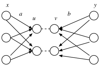
Figure 1: CCA

CCA has been proposed by Hotelling in 1935[3]. Suppose there is a pair of multi-variates ${\bf x}\in{\cal R}^{n_{x}}$ ${\bf y}\in{\cal R}^{n_{y}}$, CCA finds a pair of linear transformations such that the correlation coefficient between extracted features is maximized (Fig.1) For the sake of simplicity, we assume that the averages of ${\bf x}$ and ${\bf y}$ are 0, and the dimensionality of feature is 1, then by the transformations

$$u=\langle{\bf a},{\bf x}\rangle,$$ (1)

$$v=\langle{\bf b},{\bf y}\rangle,$$ (2)

we would like to find the transformation ${\bf a}$, ${\bf b}$ that maximizes

$$\rho={{\rm E}[uv]\over\sqrt{{\rm Var}[u]{\rm Var}[v]}},$$ (3)

where $\langle{\bf a},{\bf x}\rangle$ represents the inner product. We have to further assume

$${\rm Var}[u]={\rm Var}[v]=1,$$ (4)

to reduce the freedom of scaling of $u$ and $v$. ${\bf a}$ and ${\bf b}$ can be found by an eigen vector corresponding to the maximal eigen values of a generalized eigen value problem. If we need more than one dimension, we can take eigen vectors corresponding other maximal eigen values.

CCA is important in an information theoretical viewpoint, since it finds a transformation that maximizes the mutual information between features, when ${\bf x}$ and ${\bf y}$ are jointly Gaussian. Even if the assumption is not fullfilled, CCA can be still used in some cases. However, if the purpose is regression, the large values of correlation coefficients are crucially necessary. The reasons that correlation coefficients are small can be considered in the following cases:

1. ${\bf x}$ and ${\bf y}$ does not have almost any relation.

2. There is strong nonlinear relation between ${\bf x}$ and ${\bf y}$,

It is impossible of improvement in the first case. However, in the second case, we can obtain the relation by some methods. One of those methods is to allow the nonlinear transformation and Asoh et al[4] has proposed a neural network model that approximates the optimal nonlinear canonical correlation analysis. However, this model requires a lot of computation time and it also has a lot of local optima. In this paper, we incorporate the kernel method, which enables the nonlinear transformation as well as the small computation and no undesired local optima.

3 Kernel CCA

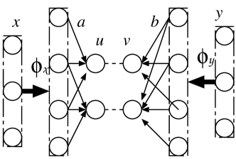
Figure 2: Kernel CCA

First, ${\bf x}$ and ${\bf y}$ are transformed into the Hilbert space, $\phi_{x}({\bf x})\in H_{x}$ and $\phi_{y}({\bf y})\in H_{y}$. By taking inner products with a parameter in the Hilbert spaces, $a\in H_{x}$, and $b\in H_{y}$, we find a feature

$$u=\langle a,\phi_{x}({\bf x})\rangle,$$ (5)

$$v=\langle b,\phi_{y}({\bf y})\rangle,$$ (6)

which maximizes the correlation coefficients.

Now, suppose we have pairs of training samples $\{({\bf x}_{i},{\bf y}_{i})\}_{i=1}^{N}$. $a$ and $b$ can be found by solving the Lagrangean

$${\cal L}_{0} = {\rm E}[(u-{\rm E}[u])(v-{\rm E}[v])]$$ (7)

$$-{\lambda_{1}\over 2}{\rm E}[(u-{\rm E}[u])^{2}]$$

$$-{\lambda_{2}\over 2}{\rm E}[(v-{\rm E}[v])^{2}].$$

However, the Lagrangean is ill-posed as it is when the dimensionalities of the Hilbert spaces are large. Therefore, we introduce a quadratic regularization term and we get well-posed Lagrangean,

$${\cal L}={\cal L}_{0}+{\eta\over 2}(\|a\|^{2}+\|b\|^{2}),$$ (8)

where $\eta$ is a regularization constant. Note that the average of $u$ is given by

$${\rm E}[u]={1\over N}\sum_{i}\langle a,\phi_{x}({\bf x}_{i})\rangle,$$ (9)

and the average of $uv$ is given by

$${\rm E}[uv]={1\over N}\sum_{i,j}\langle a,\phi_{x}({\bf x}_{i})\rangle\langle b,\phi_{y}({\bf y}_{i})\rangle.$$ (10)

Now, from the condition that the derivative of ${\cal L}$ by $a$ is equal to 0, we get

$$a=\sum_{i}\alpha_{i}\phi_{x}({\bf x}_{i}),$$ (11)

where $\alpha_{i}$ is a schalar, then as a result, we have

$$u=\sum_{i}\alpha_{i}\langle\phi_{x}({\bf x}_{i}),\phi_{x}({\bf x})\rangle.$$ (12)

Therefore, $u$ can be calculated by only inner products in $H_{x}$. Kernel trick used in SVM uses a kernel function $k_{x}({\bf x}_{1},{\bf x}_{2})$ instead of the inner product between $\phi_{x}({\bf x}_{1})$ and $\phi_{x}({\bf x}_{2})$. In practice, since we don’t need an explicit form of $\phi_{x}$, we first determine $k_{x}$ that can be decomposed in the form of inner product. From Mercer theorem, the symmetric positive definite kernel $k_{x}$ can be decomposed into the inner product form.

Let us rewrite ${\cal L}$ by the kernel. First, let ${\bf\alpha}=(\alpha_{1},$ $\ldots,$ $\alpha_{N})^{\rm T}$, ${\bf\beta}=(\beta_{1},\ldots,\beta_{N})^{\rm T}$, and we define the matrices

$$(K_{x})_{ij}=k_{x}({\bf x}_{i},{\bf x}_{j}),$$ (13)

$$(K_{y})_{ij}=k_{y}({\bf y}_{i},{\bf y}_{j}).$$ (14)

Then, we obtain ${\cal L}$ by

$${\cal L} = {\bf\alpha}^{\rm T}M{\bf\beta}$$ (15)

$$-{\lambda_{1}\over 2}{\bf\alpha}^{\rm T}L{\bf\alpha}-{\lambda_{2}\over 2}{\bf\beta}^{\rm T}N{\bf\beta}$$

where

$$M = {1\over N}K_{x}^{\rm T}JK_{y},$$ (16)

$$L = {1\over N}K_{x}^{\rm T}JK_{x}+\eta_{1}K_{x},$$ (17)

$$N = {1\over N}K_{y}^{\rm T}JK_{y}+\eta_{2}K_{y},$$ (18)

$$J = I-{1\over N}{\bf 1}{\bf 1}^{\rm T},$$ (19)

$${\bf 1} = (1,\ldots,1)^{\rm T},$$ (20)

and $\eta_{1}=\eta/\lambda_{1}$, $\eta_{2}=\eta/\lambda_{2}$.

If $\eta>0$ is satisfied, $L$ and $N$ are positive definite almost surely, and we can show $\lambda_{1}=\lambda_{2}=\lambda$ from the constraint, then as a result we have a generalized eigenvalue problem for ${\bf\alpha}$, ${\bf\beta}$

$$M{\bf\beta} = \lambda L{\bf\alpha},$$ (21)

$$M^{\rm T}{\bf\alpha} = \lambda N{\bf\beta},$$ (22)

It can be solved by generalized eigenvalue problem package or Cholesky decomposition of $L$ and $M$.

4 Computer simulation

4.1 Simulation 1

We generate training samples and test samples independently as follows. First $\theta$ is generated from the uniform distribution on $[-\pi,\pi]$, and then a pair of two dimensional variables ${\bf x}$ and ${\bf y}$ are generated by

$${\bf x}=\left(\begin{array}[]{c}\theta\\ \sin 3\theta\end{array}\right)+{\bf\epsilon}_{1},$$ (23)

$${\bf y}={\rm e}^{\theta/4}\left(\begin{array}[]{c}\cos 2\theta\\ \sin 2\theta\end{array}\right)+{\bf\epsilon}_{2},$$ (24)

where ${\bf\epsilon}_{1}$, ${\bf\epsilon}_{2}$ are independent two dimensional Gaussian noise with a standard deviation 0.05.

We test for 40 training samples and 100 test samples. The $x$–$y$ scatter plot of (linear) CCA is shown fig.3. The correlation coefficients are as follows, where the values for test samples are in the braces.

	$v_{1}$		$v_{2}$
$u_{1}$	0.71	(0.40)	0.00	(0.09)
$u_{2}$	0.00	(0.00)	0.27	(0.19)

The $x$–$y$ plot of kernel CCA is shown in fig.4. We used Gaussian kernel

$$k({\bf x}_{1},{\bf x}_{2})=\exp(-{\|{\bf x}_{1}-{\bf x}_{2}\|^{2}\over 2\sigma^{2}}),$$ (25)

both for ${\bf x}$ and ${\bf y}$, where parameters are take by $\eta=1.0$, $\sigma=1.0$. The correlation coefficients are as follows, where the values for test samples are in the braces.

	$v_{1}$		$v_{2}$
$u_{1}$	0.98	(0.95)	0.00	(0.02)
$u_{2}$	0.00	(0.02)	0.97	(0.93)

We only show upto the second components, though we have higher components in the kernel CCA.

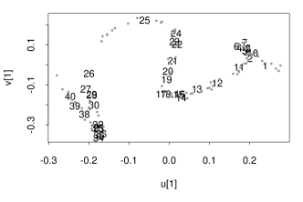
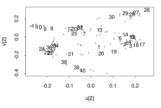
Figure 3: Simulation 1. $x$–$y$ plot for CCA. The numbers represent the increasing order of training samples for $\theta$

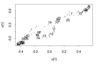
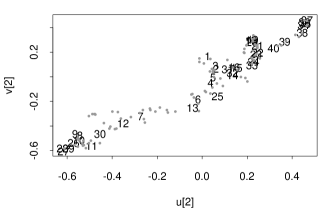
Figure 4: Simulation 1. $x$–$y$ plot for kernel CCA

4.2 Simulation 2

This section examines an artificial pattern recognition tasks in multimodal setting described in the beginning of the paper.

Training samples ${\bf x}$ and ${\bf y}$ are generated randomly from the uniform distribution on $[0,1]^{2}$ and make random pairs of training samples. Each pair of training samples represent a class center. Test samples are generated by adding an independent Gaussian noise with standard deviation 0.05 to training samples randomly chosen.

We test 10 training samples (classes) and 100 test samples.

$x$–$y$ plot of CCA result is shown in fig.5. The correlation coefficient between features are as follows, where the values for test samples are in the braces.

	$v_{1}$		$v_{2}$
$u_{1}$	0.40	(0.44)	0.00	($-$0.10)
$u_{2}$	0.00	($-$0.05)	0.13	(0.19)

$x$–$y$ plot of kernel CCA result for the same dataset is shown in fig.6.

We use Gaussian kernel in which parameters are taken $\eta=0.1$, $\sigma=0.1$. The correlation coefficients between features are as follows, where the values of test samples are in braces.

	$v_{1}$		$v_{2}$
$u_{1}$	0.97	(0.90)	0.00	(0.04)
$u_{2}$	0.00	(0.01)	0.95	(0.88)

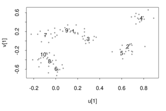
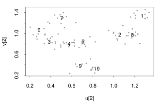
Figure 5: Simulation 2. $x$–$y$ plot of CCA. The numbers represents class centers

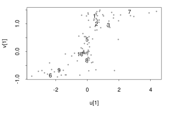
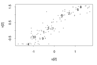
Figure 6: Simulation 2. $x$–$y$ plot of KCCA

5 Concluding remarks

5.1 Kernel method and regularization

We have proposed kernel canonial correlation analysis in which the kernel method is incorporated in the kernel method. It is similar to SVM that the point is nonlinearization by kernel method and avoiding overfitting by regularization technique.

In general, it is important to determine the regularizaion parameter. Moreover, the selection of kernel form is crucial for the performance. Although all parameters are determined by hand in the simulations of this paper, we can take more systematic approaches, such as resampling methods like cross-validation and emprical Bayes approaches[7]. In such techniques, we usually need iterative algorithms which is time consuming and is also likely to be trapped into a local optimum. To examine such issues are future work.

As for regularization term, we can use $\|{\bf\alpha}\|^{2}$ and $\|{\bf\beta}\|^{2}$ instead of the quadratic term of regularization in this paper. In the kernel discriminant analysis described below, such a different type of regularization term is used. The time complexities for both types are same and empirically we are not able to find significant difference of performance. However, we may need more realistic experiments.

5.2 Relation to kernel discriminant analysis

The canonical correlation analysis is closely related to the Fisher’s discriminant analysis (FDA), which finds a mapping that minimizes the inner-class variance as well as maximizes inter-class variance for effective pattern recognition. FDA can be considered as a special case of CCA. Mika et al[5] has proposed a kernel method for FDA, which is not strictly included into the kernel CCA because the kernel FDA does not transform the class label by nonlinear mapping. For both in kernel CCA and kernel FDA, it is difficult to obtain sparse representation of mapping. It would be promising idea to incorporate the sparsity as a utility function.

5.3 Future issues from the information theory

The author’s group has been proposed the multimodal independent component analysis (multimodal ICA) which extends the CCA by incorporating the information theoretic viewpoint[2]. The transformation is restricted to linear and it has been sometimes difficult to extract useful features from nonlinearly related multivariates. Now we can raise a question: Can we integrate the kernel CCA with multimodal ICA in order to extract useful features?

The answer for this question depends on the property of given data. If the noise level is low as in the simulation of this paper, the regularization constants are set to small values and it is desired that the correlation coefficients are almost 1. We cannot expect the performance is improved by multimodal ICA because the correlation coefficient close to 1 already achieves a large amount of mutual information.

On the other hand, when the noise level is large, the multimodal ICA possibly improves the performance. However, in such a case, the linear CCA is sometimes enough in practice. If we learn a multiple value function as in the aquisition of multiple consept[1], it may worth trying because the correlation coefficients are small even if the noise level is low.

Let us consider further the case the noise level is low. From the result of the simulations in the previous section, samples are mapped into a few clusters that will make regression between ${\bf x}$ and ${\bf y}$ difficult. In such a case, the distribution of ${\bf u}$ and ${\bf v}$ is desired to be scattered. From the information theoretic viewpoint, the feature space is preferrable to have large amount of entropy. Since the distribution with largest entropy is Gaussian under fixed average and variance, the Gaussianity can be used for the utility function. For example, the third and forth cumulants are preferrable to be as small as possible. It seems opposite from the projection pursuit and independent component analysis, but it may be caused from the difference of the purpose that ICA is for visualization while our task is for regression. The assumption of noise is also different. These issues are related to the sparsity stated in the previous section, and it is also future work.

References

- [1] S. Akaho, S. Hayamizu, O. Hasegawa, T. Yoshimura, H. Asoh: Concept aquisition from multiple information sources by the EM algorithm, Trans. of IEICE, Vol. J80-A, No. 9, pp. 1546-1553, 1997. (in Japanese; English version (ETL technical report 97-8) is available at http://www.neurosci.aist.go.jp/~akaho/papers/ETL-TR-97-8E.ps.gz)
- [2] S. Akaho and S. Umeyama, Multimodal Independent Component Analysis — A method of feature extraction from multiple information sources, Electronics and Communications in Japan, Part 3, Fundamental Electronic Science, Vol.84, No.11, pp.21–28, 2001. (summary version is available in IJCNN’99 paper, http: //www.neurosci.aist.go.jp/ ~akaho/papers/IJCNN99.ps.gz)
- [3] T. W. Anderson: An Introduction to Multivariate Statistical Analysis — Second edition, John Wiley & Sons, 1984.
- [4] H. Asoh, O. Takechi: An approximation of Nonlinear Canonical Correlation Analysis by Multilayer Perceptrons, Proc. of Int. Conf. Artificial Neural Networks, pp. 713–716, 1994.
- [5] S. Mika, G. Rätsch, J. Weston, B. Schölkpf, K-R. Müller: Fisher discriminant analysis with kernels, In Y.-H. Hu, et al.(eds.): Neural Networks for Signal Processing IX, pp. 41-48, IEEE, 1999.
- [6] B. Schölkopf, A. Smola and K. Müller: Kernel principal component analysis, In B. Schölkopf et al. (eds), Advances in Kernel Methods, Support Vector Learning, MIT Press, 1998.
- [7] M. E. Tipping: The relevant vector machine, to appear in Advances in Neural Information Processing Systems (NIPS) 12, 2000.
- [8] V.N. Vapnik : Statistical Learning Theory, John Wiley & Sons, 1998.