Coding for Additive White Noise Channels with Feedback Corrupted by Uniform Quantization or Bounded Noise

Abstract

We present simple coding strategies, which are variants of the Schalkwijk-Kailath scheme, for communicating reliably over additive white noise channels in the presence of corrupted feedback. More specifically, we consider a framework comprising an additive white forward channel and a backward link which is used for feedback. We consider two types of corruption mechanisms in the backward link. The first is quantization noise, i.e., the encoder receives the quantized values of the past outputs of the forward channel. The quantization is uniform, memoryless and time invariant (that is, symbol-by-symbol scalar quantization), with bounded quantization error. The second corruption mechanism is an arbitrarily distributed additive bounded noise in the backward link. Here we allow symbol-by-symbol encoding at the input to the backward channel. We propose simple explicit schemes that guarantee positive information rate, in bits per channel use, with positive error exponent. If the forward channel is additive white Gaussian then our schemes achieve capacity, in the limit of diminishing amplitude of the noise components at the backward link, while guaranteeing that the probability of error converges to zero as a doubly exponential function of the block length. Furthermore, if the forward channel is additive white Gaussian and the backward link consists of an additive bounded noise channel, with signal-to-noise ratio (SNR) constrained symbol-by-symbol encoding, then our schemes are also capacity-achieving in the limit of high SNR.

I Introduction

That noiseless feedback does not increase the capacity of memoryless channels, but can dramatically enhance the reliability and simplicity of the schemes that achieve it, is well known since Shannon’s work [10]. The assumption of noiseless feedback is an idealization often meant to capture communication scenarios where the noise in the backward link is significantly smaller than in the forward channel. However, all the known simple schemes for reliable communication in the presence of feedback rely heavily on the assumption that the feedback is completely noise-free, and break down when noise is introduced into the backward link.

As a case in point, it was recently shown in [5] that any feedback scheme with linear encoding (of which the Schalkwijk-Kailath scheme and its variants are special cases) breaks down completely in the presence of additive white noise of arbitrarily small variance in the backward link: not only is it impossible to achieve capacity, but, with such schemes it is impossible to communicate reliably at any positive information rate.

It is therefore of primary importance, from both the theoretical and the practical viewpoints, to develop channel coding schemes that, by making use of noisy feedback, maintain the simplicity of noiseless feedback schemes while achieving a positive rate of reliable communication. It is the quest for such schemes that motivates this paper.

Our main contribution is the derivation of simple coding strategies, which are variants of the Schalkwijk-Kailath scheme, for communicating over additive white channels in the presence of corrupted feedback. More specifically, we consider two types of corruption mechanisms in the backward link:

• Quantization noise: the encoder receives the quantized values of the past outputs of the forward channel. The quantization is uniform, memoryless and time invariant (that is, symbol-by-symbol scalar quantization), with bounded quantization error.

• Additive bounded noise: the noise in the backward link is additive, and has bounded components, but is otherwise arbitrarily distributed. Here we allow symbol-by-symbol encoding at the input to the backward channel.

The coding schemes that we present achieve positive information rate with positive error exponent. In addition, if the forward channel is additive white Gaussian then our schemes are capacity-achieving, in the limit of diminishing amplitude of the noise components in the backward link. Furthermore, if the backward link consists of an additive bounded noise channel, with instantaneous encoding, then our schemes are also capacity-achieving in the limit of high SNR (in the backward link). We note that the diminishing of the gap to capacity with vanishing noise in the backward link is a desired property, not to be taken for granted in light of the negative results in [5]. In addition, the probability of error of our coding schemes converges to zero as a doubly exponential function of the block length, provided that the forward channel is additive, white and Gaussian. As will be seen in subsequent sections, our analysis of the performance of the suggested schemes is based on elementary linear systems theory.

To our knowledge, the impact of noise in the feedback link on fundamental performance limits and on explicit schemes that attain them has hitherto received little attention. Exceptions are the papers [8, 2] which study the trade-off between reliability and delay in coding for discrete memoryless channels with noisy feedback, and suggest concrete coding schemes for this scenario. Another exception is the recent [6], which considers the capacity of discrete finite-state channels in the presence of non-invertible maps in the feedback link, such as quantization. Yet another paper is the aforementioned [5], which is primarily concerned with the impact of noise in the backward link on the error exponents.

The remainder of this paper is structured as follows. Section II presents preliminary results and definitions, while Section III specifies and analyzes a coding scheme in the presence of feedback corrupted by bounded additive noise, under the assumption that the noise is observable at the decoder. The main results of the paper are presented in Sections IV and V, where we describe and analyze coding schemes for the cases where the backward link features uniform quantization or bounded additive noise, respectively. The paper ends with conclusions in Section VI.

Notation:

• Random variables are represented in large caps, such as $Z$.

• Stochastic processes are indexed by the discrete time variable $t$, like in $X_{t}$. We also use $X^{t}$ to represent $(X_{0},\ldots,X_{t})$, provided that $t\geq 0$. If $t$ is a negative integer then we adopt the convention that $X^{t}$ is the empty set.

• A realization of a random variable $Z$ is represented in small caps, such as $z$.

II Preliminary Results and Definitions

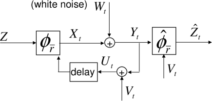
Figure 1: Basic feedback scheme.

In this Section, we define and analyze a feedback system whose structure is described by the diagram of Fig 1. The aforementioned system will be present in the coding schemes proposed in subsequent Sections.

For the remainder of this paper, we consider that $W_{t}$ is a zero mean and white stochastic process of variance $\sigma_{W}^{2}$ and that $Z$ is a real random variable taking values in $[0,1]$. In addition, $Z$ and $W^{t}$ are assumed independent for all $t$. The feedback noise $V_{t}$ is a bounded real stochastic process whose amplitude has a least upper-bound given by:

$$\bar{\sigma}_{V}\overset{def}{=}\inf\{\alpha\in\mathbb{R}_{\geq 0}:Prob(|V_{t}|>\alpha)=0,t\geq 0\}$$

meaning that the following holds:

$$Prob(|V_{t}|\leq\bar{\sigma}_{V})=1,\text{ }t\geq 0$$

The remaining signals $U_{t}$, $Y_{t}$ and $\hat{Z}_{t}$ are also real stochastic processes. The block represented in Fig 1 by $\phi_{\bar{r}}$ is an operator that maps $Z$ and $U^{t-1}$ into $X_{t}$ for all $t$. Similarly, $\hat{\phi}_{\bar{r}}$ maps $Y^{t}$ and $V^{t}$ into $\hat{Z}_{t}$. The description of the maps $\phi_{\bar{r}}$ and $\hat{\phi}_{\bar{r}}$ is given in the following definition.

Definition II.1

Given a positive real constant $\bar{r}$, the operators $\phi_{\bar{r}}:\left(t,Z,U^{t-1}\right)\mapsto X_{t}$ and $\hat{\phi}_{\bar{r}}:\left(t,Y^{t},V^{t}\right)\mapsto\hat{Z}_{t}$, represented in Fig 1, are defined as follows:

$$X_{t}=\phi_{\bar{r}}\left(t,Z,U^{t-1}\right)\overset{def}{=}\begin{cases}(2^{-\bar{r}}-2^{\bar{r}})\left(\sum_{i=0}^{t-1}2^{\bar{r}(t-i-1)}U_{i}+2^{\bar{r}t}Z\right)&\text{if $t\geq 1$}\\ (2^{-\bar{r}}-2^{\bar{r}})Z&\text{if $t=0$}\end{cases}$$ (1)

$$\hat{Z}_{t}=\hat{\phi}_{\bar{r}}\left(t,Y^{t},V^{t}\right)\overset{def}{=}\begin{cases}-\sum_{i=0}^{t-1}2^{-\bar{r}(i+1)}(V_{i}+Y_{i})&\text{ if $t\geq 1$}\\ 0&\text{if $t=0$}\end{cases}$$ (2)

Notice that (1) has a term, given by $2^{\bar{r}t}Z$, that grows exponentially. However, it should be observed that if the feedback loop is closed (see Fig 1) by using $U_{t}=X_{t}+V_{t}+W_{t}$ then $X_{t}$ is given by:

$$X_{t}=(2^{-\bar{r}}-2^{\bar{r}})\left(\sum_{i=0}^{t-1}2^{-\bar{r}(t-i-1)}(W_{i}+V_{i})+2^{-\bar{r}t}Z\right),\text{ }t\geq 1$$ (3)

which describes a system that is stable, in the bounded input implies bounded output sense. In the absence of backward link noise, i.e. $V_{t}=0$, (1) and (2) are equivalent to the equations used in the original work by Schalkwijk-Kailath [9]. An alternative minimum variance control interpretation to (1) and (2), in the presence of perfect feedback, is given in [3]. In addition, the work by [3] extends Schalkwijk-Kailath’s algorithm, with perfect feedback, to the multi-user case. A general control theoretic framework to feedback capacity is given in [11]. The following lemma states a few properties of (1) and (2) which motivate their use in the construction of coding schemes.

Lemma II.1

Let $\sigma_{W}^{2}$, $\bar{\sigma}_{V}$ and $\bar{r}$ be given positive real constants. Consider the feedback system of Fig 1, which is described by (1)-(2) in conjunction with the following equations:

$$Y_{t}=X_{t}+W_{t}$$ (4)

$$U_{t}=X_{t}+V_{t}+W_{t}$$ (5)

The following holds:

$$X_{t}=2^{\bar{r}t}(2^{\bar{r}}-2^{-\bar{r}})(\hat{Z}_{t}-Z),\text{ }t\geq 0$$ (6)

$$E[X_{t}^{2}]\leq\left(\sigma_{W}\sqrt{2^{2\bar{r}}-1}+\bar{\sigma}_{V}(2^{\bar{r}}+1)+2^{-\bar{r}t}(2^{\bar{r}}-2^{-\bar{r}})\right)^{2},\text{ }t\geq 0$$ (7)

If $W_{t}$ is zero-mean, white and Gaussian, with variance $\sigma_{W}^{2}$, then the following holds:

$$Prob\left(|X_{t}|\geq\alpha\right)\leq e^{-\frac{\left(\alpha-\gamma\right)^{2}}{2\beta^{2}}},\text{ }\alpha>0,\text{ }t\geq 0$$ (8)

where $\gamma$ and $\beta$ are the following positive real constants:

$$\gamma\overset{def}{=}\left(2^{\bar{r}}+1\right)\bar{\sigma}_{V}+2^{\bar{r}}-2^{-\bar{r}}$$ (9)

$$\beta^{2}\overset{def}{=}\left(2^{2\bar{r}}-1\right)\sigma_{W}^{2}$$ (10)

Proof: In order to derive (6), we substitute $U_{t}=V_{t}+Y_{t}$ in (2). We now proceed to proving the validity of (7). Since the operators $\phi_{\bar{r}}$ and $\hat{\phi}_{\bar{r}}$ are linear, we can bound the variance of $X_{t}$ by separately quantifying the contribution of the external inputs $Z$, $W_{t}$ and $V_{t}$. By making use of the triangular inequality, we arrive at the following bound:

$$\left(E[X_{t}^{2}]\right)^{1/2}\leq\left(\sigma_{W}^{2}\frac{1}{2\pi}\int_{-\pi}^{\pi}\left|T\left(e^{j\omega}\right)\right|^{2}d\omega\right)^{1/2}+\bar{\sigma}_{V}\max_{\omega\in(-\pi,\pi]}\left|T\left(e^{j\omega}\right)\right|+2^{-\bar{r}t}(2^{\bar{r}}-2^{-\bar{r}})$$ (11)

where $T\left(e^{j\omega}\right)$ is the following transfer function:

$$T\left(e^{j\omega}\right)=\frac{2^{-\bar{r}}-2^{\bar{r}}}{e^{j\omega}-2^{-\bar{r}}}$$ (12)

The transfer function $T\left(e^{j\omega}\right)$ describes the input-output behavior of the feedback loop from $V_{t}$ to $X_{t}$ and from $W_{t}$ to $X_{t}$. The first term in the right hand side of (11) quantifies the contribution from the white process $W_{t}$, while the second term is an upper-bound to the contribution of $V_{t}$ and the last term comes from the initial condition determined by $Z$. Standard computations lead to the following results:

$$\frac{1}{2\pi}\int_{-\pi}^{\pi}\left|T\left(e^{j\omega}\right)\right|^{2}d\omega=2^{2\bar{r}}-1$$ (13)

$$\max_{\omega\in(-\pi,\pi]}\left|T\left(e^{j\omega}\right)\right|=\frac{2^{\bar{r}}-2^{-\bar{r}}}{1-2^{-\bar{r}}}=2^{\bar{r}}+1$$ (14)

After substituting (13) and (14) in (11), we arrive at (7). In order to prove (8)-(10), under the assumption that $W_{t}$ is zero mean white Gaussian, we define the following auxiliary Gaussian process:

$$\tilde{X}_{t}=\begin{cases}0&\text{if $t=0$}\\ (2^{-\bar{r}}-2^{\bar{r}})\sum_{i=0}^{t-1}2^{-\bar{r}(t-i-1)}W_{i}&\text{if $t\geq 1$}\end{cases}$$ (15)

After simple manipulations, similar to the ones leading to (13)-(14), we get the following properties of $\tilde{X}_{t}$:

$$E[\tilde{X}_{t}^{2}]=\left(2^{2\bar{r}}-1\right)\left(1-2^{-2\bar{r}t}\right)\sigma_{W}^{2}\leq\beta^{2}$$ (16)

$$|\tilde{X}_{t}-X_{t}|\leq\left(2^{\bar{r}}-2^{-\bar{r}}\right)\left(\bar{\sigma}_{V}\frac{1-2^{-\bar{r}t}}{1-2^{-\bar{r}}}+2^{-\bar{r}t}\right)\leq\gamma$$ (17)

where we used the definitions (9) and (10) along with (3). Consequently, we arrive at:

$$Prob\left(|X_{t}|\geq\alpha\right)\leq Prob\left(|\tilde{X}_{t}|\geq\alpha-\gamma\right)\leq\sqrt{\frac{2}{\pi\beta^{2}}}\int_{\alpha-\gamma}^{\infty}e^{-\frac{\mu^{2}}{2\beta^{2}}}d\mu,\text{ }\alpha>0$$ (18)

where we used the facts that, by definition, $|\tilde{X}_{t}-X_{t}|\leq\gamma$, that $E[\tilde{X}_{t}^{2}]\leq\beta^{2}$ and that $\tilde{X}_{t}$ is normally distributed. The derivation of (8) is complete once we use the following upper-bound [7, page 220 eq. (5.1.8)]:

$$\sqrt{\frac{2}{\pi\beta^{2}}}\int_{\alpha-\gamma}^{\infty}e^{-\frac{\mu^{2}}{2\beta^{2}}}d\mu\leq e^{-\frac{\left(\alpha-\gamma\right)^{2}}{2\beta^{2}}}$$ (19)

$\square$

III A coding scheme with feedback

In this Section, we describe a coding scheme in the presence of feedback according to the framework of Fig 2, where $\phi_{\bar{r}}$ and $\hat{\phi}_{\bar{r}}$ are defined by (1)-(2), while the maps $\theta_{n,r}$ and $\hat{\theta}_{n,r}$ will be defined below. Notice that the scheme of Fig 2 assumes that $\hat{\phi}_{\bar{r}}$ has direct access to the feedback noise $V_{t}$. Under such an assumption, in this Section we construct an efficient and simple coding and decoding scheme which will be used as a basic building block in the rest of the paper. In Section IV we use the fact that if the backward link is corrupted by uniform quantization then, in fact, $V_{t}$ is the quantization error which can be recovered from the output of the forward channel and used as an input to $\hat{\phi}_{\bar{r}}$. Finally, in Section V we show that bounded noise in the feedback link can be dealt with by using a modification of the quantized feedback framework of Section IV. It should be noted that in the schemes presented in Sections IV and V, the decoder relies solely on the output of the forward channel.

The main result of this Section is stated in Theorem III.2, where we compute a rate of reliable transmission, in bits per channel use, which is achievable by the scheme of Fig 2, in the presence of a power constraint at the input of the forward channel. Such a transmission rate is a function of the parameters $\sigma_{W}^{2}$, $\bar{\sigma}_{V}$ and it also depends on the forward channel’s input power constraint, which we denote as $P_{X}^{2}$. Theorem III.2 also provides a lower bound on the error exponent of the resulting scheme. If the forward channel is additive, white and Gaussian then Theorem III.2 shows that the probability of error of the scheme of Fig 2 decreases as a doubly exponential function of the block length.

We start with the following definitions of the ceiling and floor functions denoted by $\bar{\Theta}$ and $\Theta$, respectively.

$$\bar{\Theta}(a)\overset{def}{=}\min\{n\in\mathbb{N}:a\leq n\},\text{ }a\in\mathbb{R}$$ (20)

$$\Theta(a)\overset{def}{=}\max\{n\in\mathbb{N}:a\geq n\},\text{ }a\in\mathbb{R}$$ (21)

The following definition specifies the maps $\theta_{n,r}$ and $\hat{\theta}_{n,r}$ represented in Fig 2.

Definition III.1

Given a positive integer $n$, a positive real constant $r$, a random variable $M$ taking values in the set $\{1,\ldots,2^{\Theta(rn)}\}$ and a real stochastic process $\hat{Z}_{t}$, the following is the definition of the maps $\theta_{n,r}:M\mapsto Z$ and $\hat{\theta}_{n,r}:\hat{Z}_{t}\mapsto\hat{M}_{t}$:

$$Z=\theta_{n,r}(M)\overset{def}{=}\left(M-\frac{1}{2}\right)2^{-\Theta(rn)}$$ (22)

$$\hat{M}_{t}=\hat{\theta}_{n,r}(\hat{Z}_{t})\overset{def}{=}\bar{\Theta}\left(2^{\Theta(rt)}\hat{Z}_{t}\right),\text{ }t\in\{0,\ldots,n\}$$ (23)

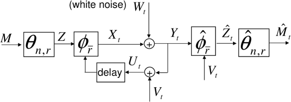
Figure 2: Basic feedback scheme with encoding and decoding.

For the remainder of this paper, $n$ denotes the block length of the coding schemes and $r$ represents a design parameter that quantifies the desired information rate, in bits per channel use. The following equations, describing the coding scheme of Fig 2, will be used in the statement of Lemma III.1 and Theorem III.2.

$$\hat{M}_{t}=\hat{\theta}_{n,r}\left(\hat{\phi}_{\bar{r}}(t,Y^{t},V^{t})\right)$$ (24)

$$Y_{t}=W_{t}+\underbrace{\phi_{\bar{r}}\left(t,\theta_{n,r}(M),U^{t-1}\right)}_{X_{t}}$$ (25)

$$U_{t}=Y_{t}+V_{t}$$ (26)

Lemma III.1

Let $\sigma_{W}^{2}$, $\bar{\sigma}_{V}$ and $\bar{r}$ be given positive real parameters. Consider that the block length is given by a positive integer $n$, that the desired transmission rate is a positive real number $r$ strictly less than $\bar{r}$ and that $M$ is a random variable arbitrarily distributed in the set $\{1,\ldots,2^{\Theta(rn)}\}$. If we adopt the scheme of Fig 2, alternatively described by (24)-(26), then the following holds:

$$Prob\left(M\neq\hat{M}_{n}\right)\leq\frac{2^{-2(\bar{r}-r)n}E[X_{n}^{2}]}{4(2^{\bar{r}}-2^{-\bar{r}})^{2}}$$ (27)

If $W_{t}$ is zero mean, white and Gaussian with variance $\sigma_{W}^{2}$ then the following doubly exponential decay, with increasing block size $n$, of the probability of error holds:

$$Prob\left(M\neq\hat{M}_{n}\right)\leq e^{-\frac{1}{2\beta^{2}}\left(2(2^{\bar{r}}-2^{-\bar{r}})2^{(\bar{r}-r)n}-\gamma\right)^{2}}$$ (28)

where $\gamma$ and $\beta$ are positive real constants given by (9) and (10), respectively.

Proof: We start by using (22)-(23) and the fact that $2^{\Theta(rn)}Z$ is in the set $\{\frac{1}{2},\ldots,2^{\Theta(rn)}-\frac{1}{2}\}$ to conclude the following:

$$\left|2^{\Theta(rn)}Z-2^{\Theta(rn)}\hat{Z}_{n}\right|<\frac{1}{2}\implies M=\hat{M}_{n}$$ (29)

leading to:

$$Prob\left(M\neq\hat{M}_{n}\right)\leq Prob\left(\left|Z-\hat{Z}_{n}\right|\geq 2^{-(\Theta(rn)+1)}\right)$$ (30)

Using (6), (30) and the fact that $\Theta(rn)\leq rn$, we get:

$$Prob\left(M\neq\hat{M}_{n}\right)\leq Prob\left(|X_{n}|\geq 2(2^{\bar{r}}-2^{-\bar{r}})2^{(\bar{r}-r)n}\right)$$ (31)

The inequality (27) follows from Markov’s inequality applied to (31). Finally, the inequality (28) follows from (31) and (8). $\square$

III-A Lower-bounds on the achievable rate of reliable transmission in the presence of a power constraint at the input of the forward channel

Below, we define a function that quantifies an achievable rate of reliable transmission for the scheme of Fig 2, in the presence of a power constraint at the input of the forward channel.

Definition III.2

For every choice of positive real parameters $\sigma_{W}^{2}$, $P_{X}^{2}$ and $\bar{\sigma}_{V}$ satisfying $4\bar{\sigma}_{V}^{2}\leq P_{X}^{2}$, define a function $\varrho:(\sigma_{W}^{2},P_{X}^{2},\bar{\sigma}_{V})\mapsto\mathbb{R}_{\geq 0}$ as the non-negative real solution $\varrho$ of the following equation:

$$\sigma_{W}\sqrt{2^{2\varrho}-1}=P_{X}-\bar{\sigma}_{V}\left(1+2^{\varrho}\right)$$ (32)

If, instead, $4\bar{\sigma}_{V}^{2}>P_{X}^{2}$ then $\varrho(\sigma_{W}^{2},P_{X}^{2},\bar{\sigma}_{V})\overset{\Delta}{=}0$.

It is readily verifiable that a non-negative real solution of (32), in terms of $\varrho$, exists and is unique, provided that $\sigma_{W}^{2}$ and $P_{X}^{2}$ are strictly positive and that $4\bar{\sigma}_{V}^{2}$ is less or equal than $P_{X}^{2}$.

Theorem III.2

Let $\sigma_{W}^{2}$, $P_{X}^{2}$ and $\bar{\sigma}_{V}$ be given positive real parameters satisfying $4\bar{\sigma}_{V}^{2}<P_{X}^{2}$. In addition, select a positive transmission rate $r$ and a positive real constant $\bar{r}$ satisfying $r<\bar{r}<\varrho(\sigma_{W}^{2},P_{X}^{2},\bar{\sigma}_{V})$. For every positive integer block length $n$ the coding scheme of Fig 2, alternatively described by (24)-(26), leads to:

$$E[X_{t}^{2}]\leq\left(P_{X}+\underbrace{2^{-\bar{r}t}(2^{\bar{r}}-2^{-\bar{r}})}_{\text{vanishes with increasing $t$}}\right)^{2},0\leq t\leq n$$ (33)

$$Prob\left(M\neq\hat{M}_{n}\right)\leq\frac{2^{-2\left(\bar{r}-r\right)n}E[X_{n}^{2}]}{4(2^{\bar{r}}-2^{-\bar{r}})^{2}}$$ (34)

where $M$ is a random variable arbitrarily distributed in the set $\{1,\ldots,2^{\Theta(nr)}\}$. If $W_{t}$ is zero mean, white and Gaussian with variance $\sigma_{W}^{2}$ then the following doubly exponential decay, with increasing block size $n$, of the probability of error holds:

$$Prob\left(M\neq\hat{M}_{n}\right)\leq e^{-\frac{1}{2\beta^{2}}\left(2(2^{\bar{r}}-2^{-\bar{r}})2^{(\bar{r}-r)n}-\gamma\right)^{2}},\text{ }\alpha>0$$ (35)

where $\gamma$ and $\beta$ are positive real constants given by (9) and (10), respectively.

Theorem III.2 shows that the scheme of Fig 2, under the constraint that the time average of the second moment of $X_{t}$ is less or equal than $P_{X}^{2}$, allows for reliable transmission at any rate $r$ strictly less than $\varrho(\sigma_{W}^{2},P_{X}^{2},\bar{\sigma}_{V})$. In addition, Theorem III.2 shows that any rate of transmission $r$, if strictly less than $\varrho(\sigma_{W}^{2},P_{X}^{2},\bar{\sigma}_{V})$, leads to an achievable error exponent arbitrarily close to $2\left[r-\varrho(\sigma_{W}^{2},P_{X}^{2},\bar{\sigma}_{V})\right]$. In addition, Theorem III.2 shows that if the forward channel is additive, white and Gaussian then the probability of error decreases with the block length $n$ at a doubly exponential rate (see (35)).

Proof of Theorem III.2: The inequalities (34) and (35) follow directly from Lemma III.1. The derivation of (33) follows from (7) and from the fact that, from Definition III.2, $\bar{r}<\varrho(\sigma_{W}^{2},P_{X}^{2},\bar{\sigma}_{V})$ implies that $\sigma_{W}\sqrt{2^{2\bar{r}}-1}+\bar{\sigma}_{V}(2^{\bar{r}}+1)<P_{X}$. $\square$

It follows from its definition, as the solution to (32), that $\varrho(\sigma_{W}^{2},P_{X}^{2},\bar{\sigma}_{V})$ also satisfies the following 3 properties:

$$\lim_{\bar{\sigma}_{V}\rightarrow 0^{+}}\varrho(\sigma_{W}^{2},P_{X}^{2},\bar{\sigma}_{V})=\frac{1}{2}\log_{2}\left(1+\frac{P_{X}^{2}}{\sigma_{W}^{2}}\right),\text{ }\sigma_{W}^{2}>0,\text{ }P_{X}^{2}>0$$ (36)

$$\varrho\left(\sigma_{W}^{2},P_{X}^{2},\frac{P_{X}^{2}}{4}\right)=0,\text{ }\sigma_{W}^{2}>0,\text{ }P_{X}^{2}>0$$ (37)

$$\varrho(\sigma_{W}^{2},P_{X}^{2},\bar{\sigma}_{V})\simeq\log_{2}\left(\frac{P_{X}}{\sigma_{W}+\bar{\sigma}_{V}}\right),\text{ }P_{X}^{2}>>\max\{\sigma_{W}^{2},\bar{\sigma}_{V}^{2}\},$$ (38)

where $\simeq$ indicates that the ratio between the left and right hand sides of (38) tends to $1$ as $P_{X}\rightarrow\infty$. If $W_{t}$ is white Gaussian then (36) indicates that in the limit, as the second moment of feedback noise goes to zero, the scheme of Fig 2 approaches capacity. We have computed $\varrho(\sigma_{W}^{2},P_{X}^{2},\bar{\sigma}_{V})$ for $\sigma_{W}^{2}=1$, $P_{X}^{2}=4$ and one thousand equally spaced values of $\bar{\sigma}_{V}$, ranging from zero to one and the results are plotted in Fig 3. The plot illustrates a graceful (continuous) degradation of $\varrho(1,4,\bar{\sigma}_{V})$ as a function of $\bar{\sigma}_{V}$, going from the highest rate of $\frac{1}{2}\log_{2}5$, achieving capacity when $W_{t}$ is Gaussian, down to zero when $\bar{\sigma}_{V}=1$, which is consistent with (36) and (37), respectively.

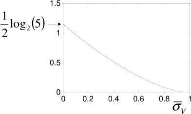
Figure 3: Plot of $\varrho(\sigma_{W}^{2},P_{X}^{2},\bar{\sigma}_{V})$ using $\sigma_{W}^{2}=1$, $P_{X}^{2}=4$ and $\bar{\sigma}_{V}\in[0,1]$.

IV Specification of a coding scheme using uniformly quantized feedback

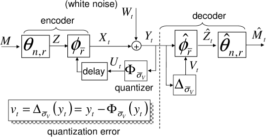
Figure 4: A coding and decoding scheme in the presence of uniformly quantized feedback.

In this Section, we consider the scheme of Fig 4, where $\Phi_{\bar{\sigma}_{V}}$ represents a memoryless uniform quantizer with sensitivity $\bar{\sigma}_{V}$ and $\Delta_{\bar{\sigma}_{V}}$ gives the associated quantization error. The main result of this Section is Corollary IV.1, where we indicate that the results of Section III hold in the presence of uniformly quantized feedback. Notice that the diagram of Fig 4 follows from Fig 2 by adopting $V_{t}$ as the quantization error, which the decoder re-constructs by making use of $\Delta_{\bar{\sigma}_{V}}$ applied to the output of the forward channel. The precise definitions of the uniform quantizer $\Phi_{\bar{\sigma}_{V}}$ and of the quantization error function $\Delta_{\bar{\sigma}_{V}}$ are given below:

Definition IV.1

Given a positive real parameter $b$, a uniform quantizer with sensitivity $b$ is a function $\Phi_{b}:\mathbb{R}\rightarrow\mathbb{R}$ defined as:

$$\Phi_{b}(y)=2b\Theta\left(\frac{y+b}{2b}\right)$$ (39)

where $\Theta$ is the floor function specified in (21). Similarly, the quantization error is given by the following function:

$$\Delta_{b}(y)=\Phi_{b}(y)-y,y\in\mathbb{R}$$ (40)

which satisfies the following bound:

$$|\Delta_{b}(y)|\leq b,y\in\mathbb{R}$$ (41)

The coding scheme of Fig 4 can be equivalently expressed by the following equations:

$$\hat{M}_{t}=\hat{\theta}_{n,r}\left(\hat{\phi}_{\bar{r}}(t,Y^{t},V^{t})\right)$$ (42)

$$Y_{t}=W_{t}+\underbrace{\phi_{\bar{r}}\left(t,\theta_{n,r}(M),U^{t-1}\right)}_{X_{t}}$$ (43)

$$U_{t}=\Phi_{\bar{\sigma}_{V}}(Y_{t})=Y_{t}+V_{t}$$ (44)

$$V_{t}=\Delta_{\bar{\sigma}_{V}}(Y_{t})$$ (45)

The Corollary below follows directly from Theorem III.2 applied to the scheme of Fig 4, along with the upper-bound (41).

Corollary IV.1

Let $\sigma_{W}^{2}$, $P_{X}^{2}$ and $\bar{\sigma}_{V}$ be positive real constants satisfying $4\bar{\sigma}_{V}^{2}<P_{X}^{2}$, where $\bar{\sigma}_{V}$ represents the sensitivity of the quantizer. In addition, select a positive transmission rate $r$ and a positive real constant $\bar{r}$ satisfying $r<\bar{r}<\varrho(\sigma_{W}^{2},P_{X}^{2},\bar{\sigma}_{V}^{2})$. For every positive integer block length $n$, the coding scheme specified by (42)-(45) (see Fig 4) leads to:

$$E[X_{t}^{2}]\leq\left(P_{X}+\underbrace{2^{-\bar{r}t}(2^{\bar{r}}-2^{-\bar{r}})}_{\text{vanishes with increasing $t$}}\right)^{2},0\leq t\leq n$$ (46)

$$Prob\left(M\neq\hat{M}_{n}\right)\leq\frac{2^{-2\left(\bar{r}-r\right)n}E[X_{n}^{2}]}{4(2^{\bar{r}}-2^{-\bar{r}})^{2}}$$ (47)

where $M$ is a random variable arbitrarily distributed in the set $\{1,\ldots,2^{\Theta(nr)}\}$. If $W_{t}$ is zero mean, white and Gaussian with variance $\sigma_{W}^{2}$ then the following doubly exponential decay, with increasing block size $n$, of the probability of error holds:

$$Prob\left(M\neq\hat{M}_{n}\right)\leq e^{-\frac{1}{2\beta^{2}}\left(2(2^{\bar{r}}-2^{-\bar{r}})2^{(\bar{r}-r)n}-\gamma\right)^{2}}$$ (48)

where $\gamma$ and $\beta$ are positive real constants given by (9) and (10), respectively.

Notice that Corollary IV.1 shows that, in the presence of uniformly quantized feedback with sensitivity $\bar{\sigma}_{V}$, any rate $r$ strictly less than $\varrho(\sigma_{W}^{2},P_{X}^{2},\bar{\sigma}_{V})$ allows for reliable transmission. This implies that the properties (36)-(37), along with the conclusions derived in Section III, hold for uniformly quantized feedback. In particular, the achievable rate of reliable transmission of the coding scheme of Fig 4 degrades gracefully as a continuous function of the quantizer sensitivity $\bar{\sigma}_{V}$ (see the numerical example portrayed in Fig 3).

V Coding and decoding in the presence of feedback corrupted by bounded noise.

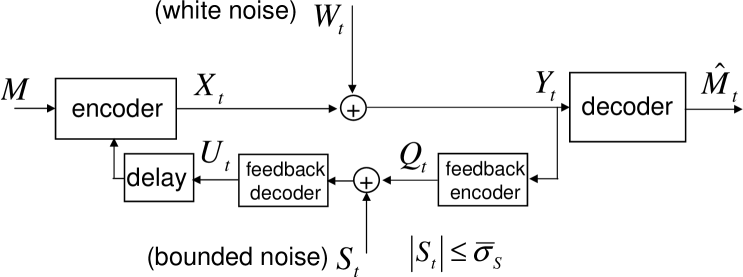
Figure 5: Communication scheme in the presence of bounded feedback noise.

From Corollary IV.1, we conclude that there exist simple explicit coding strategies based on Schalkwijk-Kailath’s framework that, even in the presence of uniformly quantized feedback, provide positive rates with positive error exponents. In this Section, we aim at designing coding schemes in the presence of feedback corrupted by bounded noise. The main result of this Section is discussed in Section V-A, where we describe a communication scheme whose structure is that of Fig 5. In addition, we analyze the performance of such a scheme in the presence of power constraints at the input of the forward and backward channels. The proposed scheme retains the simplicity of the Schalkwijk-Kailath scheme [9], but, in contrast to the original scheme (which breaks down in the presence of noise in the backward link [9, Section III.D]), achieves a positive rate of reliable communication and is in fact capacity achieving in the limit of high SNR in the backward link (assuming white Gaussian noise in the forward channel). The scheme proposed in Section V-A also guarantees that, if the forward channel is additive, white and Gaussian, then the probability of error converges to zero as a doubly exponential function of the block length. The main results of this Section are stated in Theorem V.1.

V-A Performance in the presence of a power constraint at the input of the backward channel.

For the remainder of this Section, we will define a coding scheme whose structure is that of Fig 5. The additive noise $S_{t}$ in the feedback link is arbitrarily distributed, bounded and the tightest upper-bound to its amplitude is defined below:

$$\bar{\sigma}_{S}\overset{def}{=}\inf\{\alpha\in\mathbb{R}_{\geq 0}:Prob(|S_{t}|>\alpha)=0,t\geq 0\}$$

meaning that the following holds:

$$Prob(|S_{t}|\leq\bar{\sigma}_{S})=1,\text{ }t\geq 0$$

The following remark will be used in the construction of a coding scheme with the structure of Fig 5.

Remark V.1

Let $\bar{\sigma}_{S}$ be a positive real constant and $S_{t}$ be a real valued stochastic process satisfying $|S_{t}|\leq\bar{\sigma}_{S}$ with probability one. Given a positive real parameter $\bar{\sigma}_{V}$, the following holds with probability one:

$$\frac{\bar{\sigma}_{V}}{\bar{\sigma}_{S}}\Phi_{\bar{\sigma}_{S}}\left(S_{t}+Q_{t}\right)=\Phi_{\bar{\sigma}_{V}}(Y_{t})$$ (49)

where $Q_{t}$ is given by:

$$Q_{t}=\Phi_{\bar{\sigma}_{S}}\left(\frac{\bar{\sigma}_{S}}{\bar{\sigma}_{V}}Y_{t}\right)$$ (50)

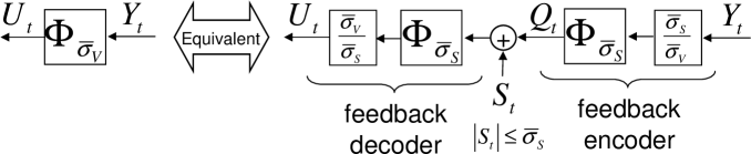
Figure 6: Schematic representation of the equivalence expressed in Remark V.1.

The schematic representation of the equivalence expressed in Remark V.1 is displayed in Fig 6. In such a scheme, $S_{t}$ is the bounded additive noise at the backward channel with input $Q_{t}$.

Aiming at constructing a coding scheme according to the structure of Fig 5, we use Remark V.1 to obtain a new coding strategy by substituting the feedback quantizer $\Phi_{\bar{\sigma}_{V}}$ of Fig 4 with the equivalent additive noise channel diagram of Fig 6. The resulting scheme, along with the encoding and decoding strategy of Section IV, provides a solution to the problem of designing encoders and decoders in the presence of an additive (bounded) noise backward channel (see Fig 7). Under such a design strategy, $\bar{\sigma}_{V}$ becomes a design parameter. Notice that viewing $\bar{\sigma}_{V}$ as a design knob is in contrast with the framework of Section IV, where $\bar{\sigma}_{V}$ was a given constant.

Regarding the role of $\bar{\sigma}_{V}$, we have shown in (36) that as $\bar{\sigma}_{V}$ approaches zero the achievable rate of reliable transmission converges to a positive value, which, in the case where $W_{t}$ is white Gaussian, coincides with capacity. However, for any given positive real $\bar{\sigma}_{S}$, the smaller $\bar{\sigma}_{V}$ the larger the scaling constant $\frac{\bar{\sigma}_{S}}{\bar{\sigma}_{V}}$ in (50) and that may lead to $Q_{t}$ having an arbitrarily large second moment. In Theorem V.1, we show that the function defined below solves the aforementioned problem by providing a suitable choice for $\sigma_{V}$, in the presence of power constraints at the input of the forward and backward channels.

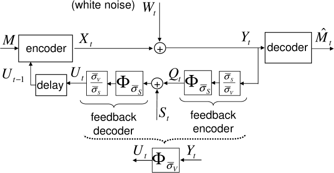
Figure 7: Proposed coding scheme for dealing with the feedback corruption that results from additive noise $S_{t}$ in the backward channel. The scheme is constructed by replacing the quantizer in the diagram of Fig 4 with the scheme of Fig 6. The encoder and decoder blocks are described in detail in Fig 4.

Definition V.1

Let $\sigma_{W}$, $\bar{\sigma}_{S}$, $P_{X}$ and $P_{Q}$ be given positive real constants, where $P_{Q}^{2}$ symbolizes a power constraint at the input of the backward channel $Q_{t}$. Below, we define the function $\Gamma:\mathbb{R}_{\geq 0}^{4}\rightarrow\mathbb{R}_{\geq 0}$, which we will use as a selection for the design parameter $\bar{\sigma}_{V}$:

$$\Gamma\left(\sigma_{W},\bar{\sigma}_{S},P_{X},P_{Q}\right)=\left(P_{X}+\sigma_{W}\right)\frac{\bar{\sigma}_{S}}{P_{Q}-\bar{\sigma}_{S}},\text{ }P_{Q}>\bar{\sigma}_{S}$$ (51)

The following Theorem is one of the main results of this paper.

Theorem V.1

Let $\sigma_{W}^{2}$, $P_{X}^{2}$, $P_{Q}^{2}$ and $\bar{\sigma}_{S}$ be positive constants satisfying $4\Gamma\left(\sigma_{W},\bar{\sigma}_{S},P_{X},P_{Q}\right)^{2}<P_{X}^{2}$ and $\bar{\sigma}_{S}<P_{Q}$. In addition, select a positive transmission rate $r$ and a positive real constant $\bar{r}$ satisfying $r<\bar{r}<\left.\varrho(\sigma_{W}^{2},P_{X}^{2},\bar{\sigma}_{V})\right|_{\bar{\sigma}_{V}=\Gamma\left(\sigma_{W},\bar{\sigma}_{S},P_{X},P_{Q}\right)}$. For every positive integer block length $n$, the coding scheme of Fig 7, alternatively described by (42)-(45) and (50), leads to:

$$E[X_{t}^{2}]\leq\left(P_{X}+\underbrace{2^{-\bar{r}t}\left(2^{\bar{r}}-2^{-\bar{r}}\right)}_{\text{vanishes with increasing $t$}}\right)^{2},\text{ }0\leq t\leq n$$ (52)

$$E[Q_{t}^{2}]\leq\left(P_{Q}+\underbrace{2^{-\bar{r}t}\frac{P_{Q}-\bar{\sigma}_{S}}{P_{X}+\sigma_{W}}\left(2^{\bar{r}}-2^{-\bar{r}}\right)}_{\text{vanishes with increasing $t$}}\right)^{2},\text{ }0\leq t\leq n$$ (53)

$$Prob\left(M\neq\hat{M}_{n}\right)\leq\frac{2^{-2\left(\bar{r}-r\right)n}E[X_{n}^{2}]}{4(2^{\bar{r}}-2^{-\bar{r}})^{2}}$$ (54)

where $M$ is a random variable arbitrarily distributed in the set $\{1,\ldots,2^{\Theta(nr)}\}$. If $W_{t}$ is zero mean, white and Gaussian with variance $\sigma_{W}^{2}$ then the following doubly exponential decay, with increasing block size $n$, of the probability of error holds:

$$Prob\left(M\neq\hat{M}_{n}\right)\leq e^{-\frac{1}{2\beta^{2}}\left(2(2^{\bar{r}}-2^{-\bar{r}})2^{(\bar{r}-r)n}-\gamma\right)^{2}}$$ (55)

where $\gamma$ and $\beta$ are positive real constants given by (9) and (10), respectively, where $\bar{\sigma}_{V}$ is given by the assumed selection $\bar{\sigma}_{V}=\Gamma\left(\sigma_{W},\bar{\sigma}_{S},P_{X},P_{Q}\right)$.

Proof: The inequalities (52), (54) and (55) follow directly from Corollary IV.1. In order to arrive at (53), we start by noticing that we can use the triangular inequality to find the following inequalities:

$$\left(E[Y_{t}^{2}]\right)^{\frac{1}{2}}\leq\left(E[X_{t}^{2}]\right)^{\frac{1}{2}}+\sigma_{W}$$ (56)

$$\left(E[Q_{t}^{2}]\right)^{\frac{1}{2}}\leq\frac{\bar{\sigma}_{S}}{\bar{\sigma}_{V}}\left(E[Y_{t}^{2}]\right)^{\frac{1}{2}}+\bar{\sigma}_{S}$$ (57)

In addition, substitution of (56) in (57), leads to:

$$E[Q_{t}^{2}]\leq\left(\frac{\bar{\sigma}_{S}}{\bar{\sigma}_{V}}\left(E[X_{t}^{2}]^{\frac{1}{2}}+\sigma_{W}\right)+\bar{\sigma}_{S}\right)^{2}$$ (58)

which, from (52), implies the following:

$$E[Q_{t}^{2}]\leq\left(\frac{\bar{\sigma}_{S}}{\bar{\sigma}_{V}}\left(P_{X}+2^{-\bar{r}t}\left(2^{\bar{r}}-2^{-\bar{r}}\right)+\sigma_{W}\right)+\bar{\sigma}_{S}\right)^{2}$$ (59)

The proof is complete since (53) follows by substituting our choice $\bar{\sigma}_{V}=\Gamma\left(\sigma_{W},\bar{\sigma}_{S},P_{X},P_{Q}\right)$ in (59). $\square$

Under the conditions of Theorem V.1, including our choice of the design parameter $\bar{\sigma}_{V}$, the following limit holds:

$$\lim_{\bar{\sigma}_{S}\rightarrow 0^{+}}\left.\varrho(\sigma_{W}^{2},P_{X}^{2},\bar{\sigma}_{V})\right|_{\bar{\sigma}_{V}=\Gamma\left(\sigma_{W},\bar{\sigma}_{S},P_{X},P_{Q}\right)}=\frac{1}{2}\log_{2}\left(1+\frac{P_{X}^{2}}{\sigma_{W}^{2}}\right),\text{ }\sigma_{W}>0,P_{X}>0,P_{Q}>0$$ (60)

Notice that (60) leads to the conclusion that, under our choice of $\bar{\sigma}_{V}$, the performance of the scheme of Theorem V.1 (see Fig 7) degrades gracefully as a function of $\bar{\sigma}_{S}$, in terms of both the rate and the error exponent. If $W_{t}$ is white Gaussian then (60) indicates that as $\bar{\sigma}_{S}$ tends to zero, the scheme of Theorem V.1 can be used to reliably communicate at a rate arbitrarily close to capacity. Moreover, such a conclusion holds in the presence of an arbitrarily low power constraint at the backward channel. The plot of Fig 8 displays how the achievable rate changes as a function of $\bar{\sigma}_{S}$, under the choice $\bar{\sigma}_{V}=\Gamma\left(\sigma_{W},\bar{\sigma}_{S},P_{X},P_{Q}\right)$. Such a plot also illustrates that by increasing $P_{Q}$ we can reduce the sensitivity of the achievable rate, of reliable transmission, relative to variations in $\bar{\sigma}_{S}$.

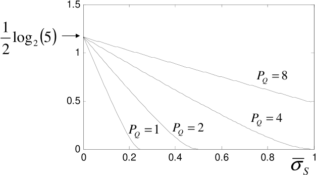
Figure 8: Plot of $\left.\varrho(\sigma_{W}^{2},P_{X}^{2},\bar{\sigma}_{V})\right|_{\bar{\sigma}_{V}=\Gamma\left(\sigma_{W},\bar{\sigma}_{S},P_{X},P_{Q}\right)}$ using $\sigma_{W}^{2}=1$, $P_{X}^{2}=4$ and $\bar{\sigma}_{S}\in[0,1)$, for $P_{Q}$ taking values $1$, $2$, $4$ and $8$.

V-B Further comments on the location of the one-step feedback delay

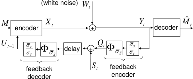
Figure 9: A coding scheme equivalent to the one described by Fig 7.

In the framework of Fig 7, the one-step delay block is located after the feedback decoder. However, we should stress that, since the feedback decoder is time-invariant, our coding scheme would be unaltered if we had placed the delay block before as indicated in Fig 9. Indeed, the diagrams of Fig 7 and 9 are equivalent, implying that Theorem V.1 holds also for the coding scheme of Fig 9.

VI Conclusions

We derived simple schemes for reliable communication over a white noise forward channel, in the presence of corrupted feedback. Both the case of uniform quantization noise and the case of additive bounded noise in the backward link were considered, where, in the latter case, encoding at the input to the backward channel is allowed. The schemes were seen to achieve a positive rate of reliable communication, and in fact be capacity-achieving in the presence of an additive white Gaussian forward channel, in the limit of small noise (or high SNR when encoding is allowed) in the backward link. In addition, still under the assumption that the forward channel is additive white Gaussian, the proposed schemes guarantee that the probability of error converges to zero as a doubly exponential function of the block length.

We believe that our approach to the construction and analysis of coding schemes carries over naturally to the case where the noise in the forward channel is non-white. In this case, we expect to obtain variations on the schemes in [4] that are analogous to those in the present work and whose gap to capacity behaves similarly.

References

- [1] T. M. Cover and J. A. Thomas; “Elements of Information Theory,” Wiley-Iterscience Publication, 1991
- [2] S. C. Draper and A. Sahai, “Noisy feedback improves communication reliability,” Proceedings of the International Symposium of Information Theory, Seattle, Washington, July 2006
- [3] N. Elia, “When Bode Meets Shannon: Control-Oriented Feedback Communication Schemes,” IEEE Transactions on Automatic Control, Vol. 49, No. 9, pp. 1477-1488, Sept. 2004
- [4] Y. H. Kim, “Feedback capacity of stationary Gaussian channels,” submitted to IEEE Transactions on Information Theory. Available at “ arxiv.org/abs/cs.IT/0602091”
- [5] Y. H. Kim, A. Lapidoth and T. Weissman, “Upper bounds on error exponents of channels with feedback,” to appear in IEEE 24th Convention of Electrical & Electronics Engineers in Israel, Eilat, Israel, November 2006
- [6] H. Permuter, T. Weissman and A. Goldsmith, “Finite State Channels with Time-Invariant Deterministic Feedback,” Available at “http://arxiv.org/abs/cs.IT/0608070”
- [7] J. G. Proakis, M. Salehi, “Fundamentals of communication systems,” Prentice Hall, 2005
- [8] A. Sahai and T. Şimşek, “On the variable-delay reliability function of discrete memoryless channels with access to noisy feedback,” Proceedings of the IEEE Information Theory Workshop, San Antonio, Texas, 2004.
- [9] J. P. M. Schalkwijk and T. Kailath, “A coding scheme for additive noise channels with feedback I: no bandwidth constraint,” IEEE Transactions on Information Theory, vol. 12, pp. 172-182, April 1966
- [10] C. E. Shannon, “The zero-error capacity of a noisy channel,” IRE Transactions on Information Theory, vol. IT-2, pp. 8–19, September 1956.
- [11] S. Yang, A. Kavcic and S. Tatikonda,“Feedback capacity of finite-state machine channels,” IEEE Transactions on Information Theory, Volume 51, Issue 3, pp. 799 –810, March 2005