High Data-Rate Single-Symbol ML Decodable Distributed STBCs for Cooperative Networks

High data-rate Distributed Orthogonal Space-Time Block Codes (DOSTBCs) which achieve the single-symbol decodability and full diversity order are proposed in this paper. An upper bound of the data-rate of the DOSTBC is derived and it is approximately twice larger than that of the conventional repetition-based cooperative strategy. In order to facilitate the systematic constructions of the DOSTBCs achieving the upper bound of the data-rate, some special DOSTBCs, which have diagonal noise covariance matrices at the destination terminal, are investigated. These codes are referred to as the row-monomial DOSTBCs. An upper bound of the data-rate of the row-monomial DOSTBC is derived and it is equal to or slightly smaller than that of the DOSTBC. Lastly, the systematic construction methods of the row-monomial DOSTBCs achieving the upper bound of the data-rate are presented.

Index Terms—Distributed space-time block codes, cooperative networks, single-symbol maximum likelihood decoding, diversity.

I Introduction

It is well-known that relay terminal cooperation can improve the performance of a wireless network considerably [1]–[4]. The basic idea of cooperative networks is that several single-antenna terminals form a distributed multi-antenna system by cooperation. Specifically, a source terminal, several relay terminals, and a destination terminal constitute a cooperative network, where the relay terminals relay the signals from the source terminal to the destination terminal. Because the destination terminal may receive different signals from several relay terminals simultaneously, some mechanism is needed to prevent or cancel the interference among these signals.

A simple solution is the so-called repetition-based cooperative strategy, which was proposed in [3]. In this strategy, only one relay terminal is allowed to transmit the signals at every time slot. Consequently, no interference exists at the destination terminal, and hence, the decoding process is single-symbol Maximum Likelihood (ML) decodable. Furthermore, it has been shown that the repetition-based cooperative strategy could achieve the full diversity order $K$, where $K$ is the number of relay terminals. Due to its single-symbol ML decodability and full diversity order, the repetition-based cooperative strategy was used and studied in many literatures [4], [6]–[10]. However, because only one relay terminal is allowed to transmitted the signals at every time slot, the repetition-based cooperative strategy can be seen as a repetition code, and hence, it has very poor bandwidth efficiency. It is easy to see that the data-rate of the repetition-based cooperative strategy is $1/K$.

Recently, many researchers noticed that the use of distributed space-time codes could improve the bandwidth efficiency of cooperative networks. In [11]–[13], the authors proved that the distributed space-time codes had higher bandwidth efficiency than the repetition-based cooperative strategy from the information theory aspect. Later on, many practical distributed space-time codes were proposed [14]–[18]. However, none of those codes were single-symbol ML decodable. In [19], Hua et al. investigated the use of the generalized orthogonal designs in cooperative networks. It is well-known that the generalized orthogonal designs can achieve single-symbol decodability and full diversity [20, 21]. However, when the generalized orthogonal designs were directly used in cooperative networks, the orthogonality of the codes was lost, and hence, the codes were not single-symbol ML decodable any more [19]. Very recently, Jing et al. used the existing orthogonal and quasi-orthogonal designs in cooperative networks and showed that they could achieve the full diversity order [22]. But, the codes proposed in [22] were not single-symbol ML decodable in general. To the best of our knowledge, high data-rate distributed space-time codes which achieve both the single-symbol ML decodability and the full diversity order have never been designed. This motivated our work.

In this paper, we propose a new type of distributed space-time codes, namely Distributed Orthogonal Space-Time Block Codes (DOSTBCs), for the amplify-and-forward cooperative networks. The proposed DOSTBCs achieve the single-symbol ML decodability and full diversity order. An upper bound of the data-rate of the DOSTBC is derived. Compared with the data-rate of the repetition-based cooperative strategy, the data-rate of the DOSTBC is approximately twice higher. However, systematic construction of the DOSTBCs achieving the upper bound of the data-rate is very hard due to the fact that the covariance matrix of the noise term at the destination terminal is non-diagonal in general. Therefore, we restrict our interests to a subset of the DOSTBCs, whose codes result in a diagonal noise covariance matrix at the destination terminal. We refer to the codes in this subset as the row-monomial DOSTBCs and derive an upper bound of the data-rate of the row-monomial DOSTBC. This upper bound is equal to or slightly smaller than that of the DOSTBC; while it is much higher than that of the repetition-based cooperative strategy. Furthermore, we develop the systematic construction methods of the row-monomial DOSTBCs achieving the upper bound of the data-rate.

The rest of this paper is organized as follows. Section II describes the cooperative network considered in this paper. In Section III, we first define the DOSTBCs and then derive an upper bound of the data-rate of the DOSTBC. In Section IV, the row-monomial DOSTBCs are first defined and an upper bound of the data-rate of the row-monomial DOSTBC is then derived. Section V presents the systematic construction methods of the DOSTBCs and row-monomial DOSTBCs achieving the upper bound of the data-rate. We present some numerical results in Section VI to evaluate the performance of the DOSTBCs and row-monomial DOSTBCs. The paper is concluded in Section VII.

Notations: Bold upper and lower letters denote matrices and row vectors, respectively. Also, $\textrm{diag}[x_{1},\cdots,x_{K}]$ denotes the $K\times K$ diagonal matrix with $x_{1},\cdots,x_{K}$ on its main diagonal; $\mbox{\boldmath$0$}_{k_{1}\times k_{2}}$ the $k_{1}\times k_{2}$ all-zero matrix; $\mbox{\boldmath$I$}_{T\times T}$ the $T\times T$ identity matrix; $\mathrm{det}(\cdot)$ the determinant of a matrix; $[\cdot]_{k}$ the $k$-th entry of a vector; $[\cdot]_{k_{1},k_{2}}$ the $(k_{1},k_{2})$-th entry of a matrix; $(\cdot)^{*}$ the complex conjugate; $(\cdot)^{H}$ the Hermitian; $(\cdot)^{T}$ the transpose. For two real numbers $a$ and $b$, $\lceil a\rceil$ denotes the ceiling function of $a$, i.e. the smallest integer bigger than $a$; $\lfloor a\rfloor$ the floor function of $a$, i.e. the largest integer smaller than $a$; $\mathrm{mod}(a,b)$ the modulo operation, i.e. $\mathrm{mod}(a,b)=a-b\lfloor a/b\rfloor$. For two sets ${\cal{S}}_{1}$ and ${\cal{S}}_{2}$, ${\cal{S}}_{1}-{\cal{S}}_{2}$ denotes the set whose elements are in ${\cal{S}}_{1}$ but not in ${\cal{S}}_{2}$.

II System Model

Consider a cooperative network with one source terminal, $K$ relay terminals, and one destination terminal. Every terminal has only one antenna and is constrained to be half-duplex, i.e. a terminal can not receive and transmit signals simultaneously. Denote the channel from the source terminal to the $k$-th relay terminal by $h_{k}$ and the channel from the $k$-th relay terminal to the destination terminal by $f_{k}$. Both $h_{k}$ and $f_{k}$ are assumed to be spatially uncorrelated complex Gaussian random variables with zero mean and unit variance. We assume that the destination terminal knows the instantaneous values of the channel coefficients $h_{k}$ and $f_{k}$ by using training sequences; while the source and relay terminals have no knowledge of the instantaneous channel coefficients.

At the beginning, the source terminal transmits $N$ complex-valued symbols over $N$ consecutive time slots. Let $\mbox{\boldmath$s$}=[s_{1},\cdots,s_{N}]$ denote the symbol vector transmitted from the source terminal, where the power of $s_{n}$ is $E_{s}$. Assume the coherence time of $h_{k}$ is larger than $N$; then the received signal vector $\mbox{\boldmath$y$}_{k}$ at the $k$-th relay terminal is given by

$$\mbox{\boldmath$y$}_{k}=h_{k}\mbox{\boldmath$s$}+\mbox{\boldmath$n$}_{k},$$ (1)

where $\mbox{\boldmath$n$}_{k}=[n_{k,1},\cdots,n_{k,N}]$ is the additive noise at the $k$-th relay terminal and is assumed to be uncorrelated complex Gaussian with zero mean and identity covariance matrix. In this paper, all the relay terminals are working in the amplify-and-forward mode and the amplifying coefficient $\rho$ is chosen to be $\sqrt{E_{r}/(1+E_{s})}$ for every relay terminal, where $E_{r}$ is the transmission power per use of every relay terminal. In order to construct a distributed space-time code, every relay terminal multiplies $\mbox{\boldmath$y$}_{k}$ and $\mbox{\boldmath$y$}_{k}^{*}$ with $\mbox{\boldmath$A$}_{k}$ and $\mbox{\boldmath$B$}_{k}$, respectively, and then sum up these two products. The dimension of $\mbox{\boldmath$A$}_{k}$ and $\mbox{\boldmath$B$}_{k}$ is $N\times T$. Thus, the transmitted signal vector $\mbox{\boldmath$x$}_{k}$ from the $k$-th relay terminal is given by

$$\mbox{\boldmath$x$}_{k} = \rho(\mbox{\boldmath$y$}_{k}\mbox{\boldmath$A$}_{k}+\mbox{\boldmath$y$}_{k}^{*}\mbox{\boldmath$B$}_{k})$$ (2)

$$= \rho h_{k}\mbox{\boldmath$s$}\mbox{\boldmath$A$}_{k}+\rho h_{k}^{*}\mbox{\boldmath$s$}^{*}\mbox{\boldmath$B$}_{k}+\rho\mbox{\boldmath$n$}_{k}\mbox{\boldmath$A$}_{k}+\rho\mbox{\boldmath$n$}_{k}^{*}\mbox{\boldmath$B$}_{k}.$$

Assume the coherence time of $f_{k}$ is larger than $T$; then the received signal vector $\mbox{\boldmath$y$}_{D}$ at the destination terminal is given by

$$\mbox{\boldmath$y$}_{D} = \sum_{k=1}^{K}f_{k}\mbox{\boldmath$x$}_{k}+\mbox{\boldmath$n$}_{D}$$ (3)

$$= \sum_{k=1}^{K}(\rho f_{k}h_{k}\mbox{\boldmath$s$}\mbox{\boldmath$A$}_{k}+\rho f_{k}h_{k}^{*}\mbox{\boldmath$s$}^{*}\mbox{\boldmath$B$}_{k})+\sum_{k=1}^{K}(\rho f_{k}\mbox{\boldmath$n$}_{k}\mbox{\boldmath$A$}_{k}+\rho f_{k}\mbox{\boldmath$n$}_{k}^{*}\mbox{\boldmath$B$}_{k})+\mbox{\boldmath$n$}_{D},$$

where $\mbox{\boldmath$n$}_{D}=[n_{D,1},\cdots,n_{D,T}]$ is the additive noise at the destination terminal and is assumed to be uncorrelated complex Gaussian with zero mean and identity covariance matrix. Define $w$, $X$, and $n$ as follows:

$$w = [\rho f_{1},\cdots,\rho f_{K}]$$ (4)

$$X = [h_{1}\mbox{\boldmath$s$}\mbox{\boldmath$A$}_{1}+h_{1}^{*}\mbox{\boldmath$s$}^{*}\mbox{\boldmath$B$}_{1},\cdots,h_{K}\mbox{\boldmath$s$}\mbox{\boldmath$A$}_{K}+h_{K}^{*}\mbox{\boldmath$s$}^{*}\mbox{\boldmath$B$}_{K}]^{T}$$ (5)

$$n = \sum_{k=1}^{K}(\rho f_{k}\mbox{\boldmath$n$}_{k}\mbox{\boldmath$A$}_{k}+\rho f_{k}\mbox{\boldmath$n$}_{k}^{*}\mbox{\boldmath$B$}_{k})+\mbox{\boldmath$n$}_{D};$$ (6)

then we can rewrite (3) in the following way

$$\mbox{\boldmath$y$}_{D}=\mbox{\boldmath$w$}\mbox{\boldmath$X$}+\mbox{\boldmath$n$}.$$ (7)

Because the matrix $X$ contains $N$ information-bearing symbols, $s_{1},\cdots,s_{N}$, and it lasts for $T$ time slots, the data-rate of $X$ is equal to $N/T$. From (6), it is easy to see that the mean of $n$ is zero and the covariance matrix $\mbox{\boldmath$R$}={\mathrm{E}}\left\{\mbox{\boldmath$n$}^{H}\mbox{\boldmath$n$}\right\}$ of $n$ is given by

$$R = \sum_{k=1}^{K}\left(|\rho f_{k}|^{2}\left(\mbox{\boldmath$A$}_{k}^{H}\mbox{\boldmath$A$}_{k}+\mbox{\boldmath$B$}_{k}^{H}\mbox{\boldmath$B$}_{k}\right)\right)+\mbox{\boldmath$I$}_{T\times T}.$$ (8)

III Distributed Orthogonal Space-Time Block Codes

In this section, we will define the DOSTBCs at first. Then, in order to derive an upper bound of the data-rate of the DOSTBC, some conditions on $\mbox{\boldmath$A$}_{k}$ and $\mbox{\boldmath$B$}_{k}$ are presented. Lastly, based on those conditions, the upper bound is derived.

From (7), the ML estimate $\hat{\mbox{\boldmath$s$}}$ of $s$ is given by

$$\hat{\mbox{\boldmath$s$}} = \arg\min_{{\scriptsize\mbox{\boldmath$s$}}\in{\cal{C}}}(\mbox{\boldmath$y$}_{D}-\mbox{\boldmath$w$}\mbox{\boldmath$X$})\mbox{\boldmath$R$}^{-1}(\mbox{\boldmath$y$}_{D}-\mbox{\boldmath$w$}\mbox{\boldmath$X$})^{H}$$ (9)

$$= \arg\min_{{\scriptsize\mbox{\boldmath$s$}}\in{\cal{C}}}\left(-2\Re\left(\mbox{\boldmath$w$}\mbox{\boldmath$X$}\mbox{\boldmath$R$}^{-1}\mbox{\boldmath$y$}_{D}^{H}\right)+\mbox{\boldmath$w$}\mbox{\boldmath$X$}\mbox{\boldmath$R$}^{-1}\mbox{\boldmath$X$}^{H}\mbox{\boldmath$w$}^{H}\right),$$

where ${\cal{C}}$ is the set containing all the possible symbol vector $s$ and it depends on the modulation scheme of $s_{n}$. Inspired by the definition of the generalized orthogonal designs [21, 23], we define the DOSTBCs in the following way.

Definition 1: A $K\times T$ matrix $X$ is called a Distributed Orthogonal Space-Time Block Code (DOSTBC) in variables $s_{1},\cdots,s_{N}$ if the following two conditions are satisfied:

D1.1)

The entries of $X$ are 0, $\pm h_{k}s_{n}$, $\pm h_{k}^{*}s_{n}^{*}$, or multiples of these indeterminates by j, where $\textbf{j}=\sqrt{-1}$.

D1.2)

The matrix $X$ satisfies the following equality

$$\mbox{\boldmath$X$}\mbox{\boldmath$R$}^{-1}\mbox{\boldmath$X$}^{H} = |s_{1}|^{2}\mbox{\boldmath$D$}_{1}+\cdots+|s_{N}|^{2}\mbox{\boldmath$D$}_{N},$$ (10)

where $\mbox{\boldmath$D$}_{n}$ is

$$\mbox{\boldmath$D$}_{n} = {\mathrm{diag}}[|h_{1}|^{2}D_{n,1},\cdots,|h_{K}|^{2}D_{n,K}]$$ (11)

and $D_{n,1},\cdots,D_{n,K}$ are non-zero.

Substituting (10) into (9), it is easy to show that the DOSTBCs are single-symbol ML decodable. Furthermore, the numerical results given in Section VI will demonstrate that the DOSTBCs can achieve the full diversity order $K$. Therefore, compared with the repetition-based cooperative strategy, the DOSTBCs have the same decoding complexity and diversity order. In this paper, we will show that the DOSTBCs have much better bandwidth efficiency than the repetition-based cooperative strategy.

In order to show the higher bandwidth efficiency of the DOSTBCs, it is desirable to derive an upper bound of the data-rate of the DOSTBC. Generally, it is very hard to derive the upper bound by directly using the conditions on $X$ in Definition 1. From (5), we note that the structure of $X$ is purely decided by $\mbox{\boldmath$A$}_{k}$ and $\mbox{\boldmath$B$}_{k}$. Therefore, we transfer the conditions on $X$ into some conditions on $\mbox{\boldmath$A$}_{k}$ and $\mbox{\boldmath$B$}_{k}$. We first present some fundamental conditions on $\mbox{\boldmath$A$}_{k}$ and $\mbox{\boldmath$B$}_{k}$ from D1.1, which will be used throughout this paper. For convenience, we define that a matrix is said to be column-monomial (row-monomial) if there is at most one non-zero entry on every column (row) of it.

Lemma 1

If a DOSTBC $X$ in variables $s_{1},\cdots,s_{N}$ exists, its associated matrices $\mbox{\boldmath$A$}_{k}$ and $\mbox{\boldmath$B$}_{k}$, $1\leq k\leq K$, satisfy the following conditions:

1. The entries of $\mbox{\boldmath$A$}_{k}$ and $\mbox{\boldmath$B$}_{k}$ can only be 0, $\pm 1$, or $\pm\textbf{j}$.

2. $\mbox{\boldmath$A$}_{k}$ and $\mbox{\boldmath$B$}_{k}$ can not have non-zero entries at the same position.

3. $\mbox{\boldmath$A$}_{k}$, $\mbox{\boldmath$B$}_{k}$, and $\mbox{\boldmath$A$}_{k}+\mbox{\boldmath$B$}_{k}$ are column-monomial.

Proof:

See Appendix A. ∎

Secondly, we derive some conditions on $\mbox{\boldmath$A$}_{k}$ and $\mbox{\boldmath$B$}_{k}$ that are equivalent with the orthogonal condition (10) on $X$.

Lemma 2

The orthogonal condition (10) on $X$ holds if and only if

$$\mbox{\boldmath$A$}_{k_{1}}\mbox{\boldmath$R$}^{-1}\mbox{\boldmath$A$}_{k_{2}}^{H} = \mbox{\boldmath$0$}_{N\times N},\hskip 56.9055pt1\leq k_{1}\neq k_{2}\leq K$$ (12)

$$\mbox{\boldmath$B$}_{k_{1}}\mbox{\boldmath$R$}^{-1}\mbox{\boldmath$B$}_{k_{2}}^{H} = \mbox{\boldmath$0$}_{N\times N},\hskip 56.9055pt1\leq k_{1}\neq k_{2}\leq K$$ (13)

$$\mbox{\boldmath$A$}_{k_{1}}\mbox{\boldmath$R$}^{-1}\mbox{\boldmath$B$}_{k_{2}}^{H}+\mbox{\boldmath$B$}_{k_{2}}^{*}\mbox{\boldmath$R$}^{-1}\mbox{\boldmath$A$}_{k_{1}}^{T} = \mbox{\boldmath$0$}_{N\times N},\hskip 56.9055pt1\leq k_{1},k_{2}\leq K$$ (14)

$$\mbox{\boldmath$B$}_{k_{1}}\mbox{\boldmath$R$}^{-1}\mbox{\boldmath$A$}_{k_{2}}^{H}+\mbox{\boldmath$A$}_{k_{2}}^{*}\mbox{\boldmath$R$}^{-1}\mbox{\boldmath$B$}_{k_{1}}^{T} = \mbox{\boldmath$0$}_{N\times N},\hskip 56.9055pt1\leq k_{1},k_{2}\leq K$$ (15)

$$\mbox{\boldmath$A$}_{k}\mbox{\boldmath$R$}^{-1}\mbox{\boldmath$A$}_{k}^{H}+\mbox{\boldmath$B$}^{*}_{k}\mbox{\boldmath$R$}^{-1}\mbox{\boldmath$B$}^{T}_{k} = {\mathrm{diag}}[D_{1,k},\cdots,D_{N,k}],\hskip 56.9055pt1\leq k\leq K.$$ (16)

Proof:

See Appendix B. ∎

One possible way to derive the upper bound of the data-rate of the DOSTBC is by using the conditions (12)–(16) in Lemma 2. However, the existence of $\mbox{\boldmath$R$}^{-1}$ in those conditions make the derivation very hard. Therefore, we simplify the conditions (12)–(16) in the following theorem by eliminating $\mbox{\boldmath$R$}^{-1}$.

Theorem 1

If a DOSTBC $X$ in variables $s_{1},\cdots,s_{N}$ exists, we have

$$\mbox{\boldmath$X$}\mbox{\boldmath$X$}^{H} = |s_{1}|^{2}\mbox{\boldmath$E$}_{1}+\cdots+|s_{N}|^{2}\mbox{\boldmath$E$}_{N},$$ (17)

where $\mbox{\boldmath$E$}_{n}$ is

$$\mbox{\boldmath$E$}_{n} = {\mathrm{diag}}[|h_{1}|^{2}E_{n,1},\cdots,|h_{K}|^{2}E_{n,K}]$$ (18)

and $E_{n,1},\cdots,E_{n,K}$ are strictly positive.

Proof:

See Appendix C. ∎

Theorem 1 can provide some intuitive explanations on the full diversity of the DOSTBCs. According to Theorem 1, $E_{n,1},\cdots,E_{n,K}$, $1\leq n\leq N$, are strictly positive for a DOSTBC $X$. This implies that every row of $X$ has at least one entry containing $s_{n}$, or equivalently, every relay terminal transmits at least one symbol containing $s_{n}$, $1\leq n\leq N$. Therefore, the destination terminal receives $K$ replica of $s_{n}$ through $K$ independent fading channels and the diversity order of the DOSTBCs should be $K$.

Furthermore, the new orthogonal condition (17) on $X$ and its equivalent conditions (C.1)–(C.5) on $\mbox{\boldmath$A$}_{k}$ and $\mbox{\boldmath$B$}_{k}$ are much simpler than the original orthogonal condition (10) and its equivalent conditions (12)–(16). The new conditions enable us to find an upper bound of the data-rate of the DOSTBC.

Theorem 2

If a DOSTBC $X$ in variables $s_{1},\cdots,s_{N}$ exists, its data-rate $\mathrm{Rate}$ satisfies the following inequality:

$${\mathrm{Rate}}=\frac{N}{T}\leq\frac{N}{\lceil\frac{NK}{2}\rceil}.$$ (19)

Proof:

See Appendix D. ∎

Compared with the data-rate $1/K$ of the repetition-based cooperative strategy, it is easy to see that the upper bound of (19) is approximately twice higher, which implies that the DOSTBCs potentially have much higher bandwidth efficiency over the repetition-based cooperative strategy. Furthermore, it is worthy of addressing that the DOSTBCs have the same decoding complexity and diversity order as the repetition-based cooperative strategy.

After obtaining the upper bound of the data-rate of the DOSTBC, a natural question is how to construct the DOSTBCs achieving the upper bound of (19). Unfortunately, only for the case that $N$ and $K$ are both even, we can find such DOSTBCs and they are given in Subsection V-A. For the other cases, where $N$ or/and $K$ is odd, we could not find any DOSTBCs achieving the upper bound of (19). We note that the major hindrance comes from the fact that the noise covariance matrix $R$ in (8) is not diagonal in general. In the next section, thus, we will consider a subset of the DOSTBCs, whose codes result in a diagonal $R$.

IV Row-Monomial Distributed Orthogonal Space-Time Block Codes

In this section, we first show that, if $\mbox{\boldmath$A$}_{k}$ and $\mbox{\boldmath$B$}_{k}$ are row-monomial, the covariance matrix $R$ becomes diagonal. Then we define a subset of the DOSTBCs, whose associated matrices $\mbox{\boldmath$A$}_{k}$ and $\mbox{\boldmath$B$}_{k}$ are row-monomial, and hence, we refer to the codes in this subset as the row-monomial DOSTBCs. Lastly, an upper bound of the data-rate of the row-monomial DOSTBC is derived.

As we stated in Section III, the non-diagonality of $R$ makes the construction of the DOSTBCs achieving the upper-bound of (19) very hard. Thus, we restrict our interests to a special subset of the DOSTBCs, where $R$ is diagonal. In the following, we show that the diagonality of $R$ is equivalent with the row-monomial condition of $\mbox{\boldmath$A$}_{k}$ and $\mbox{\boldmath$B$}_{k}$.

Theorem 3

The matrix $R$ in (8) is a diagonal matrix if and only if $\mbox{\boldmath$A$}_{k}$ and $\mbox{\boldmath$B$}_{k}$ are row-monomial.

Proof:

See Appendix E. ∎

Based on Theorem 3, we define the row-monomial DOSTBCs in the following way.

Definition 2: A $K\times T$ matrix $X$ is called a row-monomial DOSTBC in variables $s_{1},\cdots,s_{N}$ if it satisfies D1.1 and D1.2 in Definition 1 and its associated matrices $\mbox{\boldmath$A$}_{k}$ and $\mbox{\boldmath$B$}_{k}$, $1\leq k\leq K$, are both row-monomial.

Obviously, the row-monomial DOSTBCs are single-symbol ML decodable because they are in a subset of the DOSTBCs. Numerical results in Section VI show that they also achieve the full diversity order $K$. Furthermore, all the results in Section III are still valid for the row-monomial DOSTBCs. In particular, the upper-bound given by (19) can still serve as an upper-bound of the data-rate of the row-monomial DOSTBC. However, due to some special properties of the row-monomial DOSTBCs, a tighter upper bound can be derived. To this end, we need to present several conditions on $\mbox{\boldmath$A$}_{k}$ and $\mbox{\boldmath$B$}_{k}$ at first. In this paper, two matrices $A$ and $B$ are said to be column-disjoint, if $A$ and $B$ can not contain non-zero entries on the same column simultaneously, i.e. if a column in $A$ contains a non-zero entry at any row, then all the entries of the same column in $B$ must be zero; conversely, if a column in $B$ contains a non-zero entry at any row, then all the entries of the same column in $A$ must be zero.

Lemma 3

If a row-monomial DOSTBC $X$ in variables $s_{1},\cdots,s_{N}$ exists, its associated matrices $\mbox{\boldmath$A$}_{k}$ and $\mbox{\boldmath$B$}_{k}$, $1\leq k\leq K$, satisfy the following two conditions:

1) $\mbox{\boldmath$A$}_{k_{1}}$ and $\mbox{\boldmath$A$}_{k_{2}}$ are column-disjoint for $k_{1}\neq k_{2}$.

2) $\mbox{\boldmath$B$}_{k_{1}}$ and $\mbox{\boldmath$B$}_{k_{2}}$ are column-disjoint for $k_{1}\neq k_{2}$.

Proof:

See Appendix F. ∎

Lemma 3 is crucial to find the upper bound of the data-rate of the row-monomial DOSTBC. According to Definition 2, if $X$ is a row-monomial DOSTBC, there are two types of non-zero entries in it: 1) the entries containing $\pm h_{k}s_{n}$ or the multiples of it by j; 2) the entries containing $\pm h_{k}^{*}s_{n}^{*}$ or the multiples of it by j. In the following, we will refer to the first type of entries as the non-conjugate entries and refer to the second type of entries as the conjugate entries. Lemma 3 implies that any column in $X$ can not contain more than one non-conjugate entry or more than one conjugate entries. However, one column in $X$ can contain one non-conjugate entry and one conjugate entry at the same time. Therefore, the columns in $X$ can be partitioned into two types: 1) the columns containing one non-conjugate entry or one conjugate entry; 2) the columns containing one non-conjugate entry and one conjugate entry. In the following, we will refer to the first type of columns as the Type-I columns and refer to the second type of columns as the Type-II columns. For the Type-II columns, we have the following lemma.

Lemma 4

If a row-monomial DOSTBC $X$ in variables $s_{1},\cdots,s_{N}$ exists, the Type-II columns in $X$ have the following properties:

1. The total number of the Type-II columns in $X$ is even.

2. In all the Type-II columns of $X$, the total number of the entries containing $s_{n}$ or $s_{n}^{*}$, $1\leq n\leq N$, is even.

Proof:

See Appendix G. ∎

Since the data-rate of $X$ is defined as $N/T$, improving the data-rate of $X$ is equivalent to reducing the length $T$ of $X$, when $N$ is fixed. Furthermore, we note that a Type-II column contains two non-zero entries; while a Type-I column contains only one non-zero entries. Therefore, if all the non-zero entries in $X$ are contained in the Type-II columns, the data-rate of $X$ achieves the maximum value. Unfortunately, in some circumstances, not all the non-zero entries in $X$ can be contained in the Type-II columns. In those circumstances, in order to reduce $T$, we need to make $X$ contain non-zero entries in the Type-II columns as many as possible. Based on this and Lemmas 3 and 4, we derive an upper bound of the data-rate of the row-monomial DOSTBC and the result is given in the following theorem.

Theorem 4

If a row-monomial DOSTBC $X$ in variables $s_{1},\cdots,s_{N}$ exists, its data-rate ${\mathrm{Rate}}_{r}$ satisfies the following inequality:

$${\mathrm{Rate}}_{r}=\frac{N}{T}\leq\left\{\begin{array}[]{cl}\frac{1}{m},&{\mathrm{when}}\hskip 8.53581ptN=2l,K=2m\\ \frac{2l+1}{2lm+2m},&{\mathrm{when}}\hskip 8.53581ptN=2l+1,K=2m\\ \frac{1}{m+1},&{\mathrm{when}}\hskip 8.53581ptN=2l,K=2m+1\\ \min\left(\frac{2l+1}{2lm+2m+l+1},\frac{2l+1}{2lm+2l+m+1}\right),&{\mathrm{when}}\hskip 8.53581ptN=2l+1,K=2m+1\\ \end{array}\right.,$$ (20)

where $l$ and $m$ are positive integers.

Proof:

See Appendix H. ∎

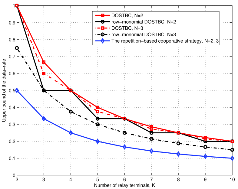
Figure 1: Comparison of the upper bounds of the data-rates of the DOSTBC, row-monomial DOSTBC, and repetition-based cooperative strategy, $N=2$, $3$.

According to (20), the row-monomial DOSTBCs have much better bandwidth efficiency than the repetition-based cooperative strategy. In order to compare the bandwidth efficiency of the DOSTBCs and row-monomial DOSTBCs, we summarize the upper bounds given by (19) and (20) in Fig. 1 and Table I. For the first case that $N$ and $K$ are even, the upper bounds of the data-rates of the DOSTBC and row-monomial DOSTBC are both $1/m$, i.e. they have the same bandwidth efficiency. A systematic method to construct the DOSTBCs and row-monomial DOSTBCs achieving the upper bound $1/m$ is given in Subsection V-A. For the other three cases, the upper bound of the data-rate of the row-monomial DOSTBC is smaller than that of the DOSTBC. However, the difference is very marginal and it goes to zero asymptotically when $K$ goes to infinite. Therefore, when a large number of relay terminals participate in the cooperation, the row-monomial DOSTBCs will have almost the same bandwidth efficiency as the DOSTBCs. Furthermore, systematic construction methods of the row-monomial DOSTBCs achieving the upper bound of (20) are given in Subsections V-B, V-C and V-D for these three cases.

Actually, we conjecture that the upper bound of (19) can be tightened for those three cases and it should be the same as (20) irrespective of the values of $N$ and $K$. The proof has not been found yet; but we provide some intuitive reasons in the following. As we mentioned before, any column in a row-monomial DOSTBC can not contain more than two non-zero entries due to the row-monomial condition of $\mbox{\boldmath$A$}_{k}$ and $\mbox{\boldmath$B$}_{k}$. On the other hand, one column in a DOSTBC can contain at most $K$ non-zero entries. However, including more than two non-zero entries in one column may be harmful to the maximum data-rate. Let us consider the following example. Assume the first column of $X$ contains three non-zero entries at the first, second, and third row. Without loss of generality, those non-zero entries are assumed to be $h_{1}s_{n_{1}}$, $h_{2}^{*}s_{n_{2}}^{*}$, and $h_{3}s_{n_{3}}$. Thus, in order to make the first and third row orthogonal with each other, there must be another column containing $-h_{1}s_{n_{1}}$ and $h_{3}s_{n_{3}}$ at the first and third row, respectively. Therefore, there are two non-zero entries at the first row of $X$ containing $s_{n_{1}}$ and it is detrimental to the data-rate of $X$. As in this example, including three non-zero entries in one column will make two non-zero entries at one row contain the same symbol, and hence, it will decrease the data-rate. The same argument can be made when more than three non-zero entries are included in one column. Therefore, we believe that including more than two non-zero entries in one column will incur a loss of the data-rate of the code. Since the row-monomial DOSTBCs never contain more than two non-zero entries in one column, we conjecture that the upper bound of the data-rate of the row-monomial DOSTBC should be the upper bound of the data-rate of the DOSTBC as well.

V Systematic Construction of the DOSTBCs and Row-Monomial DOSTBCs Achieving the Upper Bound of the Data-Rate

In this section, we present the systematic construction methods of the DOSTBCs and row-monomial DOSTBCs achieving the upper bound of the data-rate. For given $N$ and $K$, we use $\mbox{\boldmath$X$}(N,K)$ to denote the codes achieving the upper bound of the data-rate. There are four different cases depending on the values of $N$ and $K$.

V-A $N=2l$ and $K=2m$

For this case, the systematic construction method of the DOSTBCs achieving the upper bound of (19) is found. For convenience, we will use $\mbox{\boldmath$A$}_{k}(:,t_{1}:t_{2})$ to denote the submatrix consisting of the $t_{1}$-th, $t_{1}+1$-th, $\cdots$, $t_{2}$-th columns of $\mbox{\boldmath$A$}_{k}$. Similarly, $\mbox{\boldmath$B$}_{k}(:,t_{1}:t_{2})$ denotes the submatrix consisting of the $t_{1}$-th, $t_{1}+1$-th, $\cdots$, $t_{2}$-th columns of $\mbox{\boldmath$B$}_{k}$. Furthermore, define $\mbox{\boldmath$G$}_{s}$ as follows:

$$\mbox{\boldmath$G$}_{s} = \left[\begin{array}[]{cc}0&1\\ 1&0\\ \end{array}\right].$$ (23)

Based on $\mbox{\boldmath$G$}_{s}$, two matrices $\mbox{\boldmath$G$}_{A}$ and $\mbox{\boldmath$G$}_{B}$ with dimension $N\times N$ are defined:

$$\mbox{\boldmath$G$}_{A} = {\mathrm{diag}}[1,-1,1,-1,\cdots,1,-1]$$ (24)

$$\mbox{\boldmath$G$}_{B} = {\mathrm{diag}}\left[\mbox{\boldmath$G$}_{s},\cdots,\mbox{\boldmath$G$}_{s}\right].$$ (25)

The proposed systematic construction method of the DOSTBCs achieving the upper bound of (19) is as follows:

Construction I:

Initialization: Set $p=1$. Set $\mbox{\boldmath$A$}_{k}=\mbox{\boldmath$B$}_{k}=\mbox{\boldmath$0$}_{N\times\infty}$, $1\leq k\leq K$, where $\infty$ means that the length of the matrices is not decided yet.

Step 1: Set $\mbox{\boldmath$A$}_{2p-1}(:,(p-1)N+1:pN)=\mbox{\boldmath$G$}_{A}$ and $\mbox{\boldmath$B$}_{2p}(:,(p-1)N+1:pN)=\mbox{\boldmath$G$}_{B}$.

Step 2: Set $p=p+1$. If $p\leq m$, go to Step 1; otherwise, go to Step 3.

Step 3: Discard the all-zero columns at the tail of $\mbox{\boldmath$A$}_{K-1}$ and $\mbox{\boldmath$B$}_{K}$. Set the length of $\mbox{\boldmath$A$}_{k}$ and $\mbox{\boldmath$B$}_{k}$, $1\leq k\leq K$, equal to that of $\mbox{\boldmath$A$}_{K-1}$ and $\mbox{\boldmath$B$}_{K}$.

Step 4: Calculate $\mbox{\boldmath$X$}(N,K)$ through (5) by using the matrices $\mbox{\boldmath$A$}_{k}$ and $\mbox{\boldmath$B$}_{k}$ obtained in Steps 1–3, and end the construction.

The following lemma shows that Construction I generates the DOSTBCs achieving the upper bound of (19) for any even $N$ and $K$.

Lemma 5

For any even $N=2l$ and $K=2m$, the codes generated by Construction I achieve the data-rate $1/m$.

Proof:

In Construction I, the length of $\mbox{\boldmath$A$}_{k}$ and $\mbox{\boldmath$B$}_{k}$, $1\leq k\leq K$, is decided by the length of $\mbox{\boldmath$A$}_{K-1}$ and $\mbox{\boldmath$B$}_{K}$. Because $\mbox{\boldmath$A$}_{K-1}(:,(m-1)N+1:mN)$ and $\mbox{\boldmath$B$}_{K}(:,(m-1)N+1:mN)$ are set to be $\mbox{\boldmath$G$}_{A}$ and $\mbox{\boldmath$G$}_{B}$, respectively, when $p=m$, the length of $\mbox{\boldmath$A$}_{K-1}$ and $\mbox{\boldmath$B$}_{K}$ is $mN$. Consequently, the length of $\mbox{\boldmath$A$}_{k}$ and $\mbox{\boldmath$B$}_{k}$, $1\leq k\leq K$ is $mN$. By (5), the length of $\mbox{\boldmath$X$}(N,K)$ is $T$ and it is the same as that of $\mbox{\boldmath$A$}_{k}$ and $\mbox{\boldmath$B$}_{k}$. Therefore, the value of $T$ is $mN$, and hence, the data-rate of $\mbox{\boldmath$X$}(N,K)$ is $1/m$. ∎

For example, when $N=4$ and $K=4$, the code constructed by Construction I is given by

$$\mbox{\boldmath$X$}(4,4) = \left[\begin{array}[]{cccccccc}h_{1}s_{1}&-h_{1}s_{2}&h_{1}s_{3}&-h_{1}s_{4}&0&0&0&0\\ h_{2}^{*}s_{2}^{*}&h_{2}^{*}s_{1}^{*}&h_{2}^{*}s_{4}^{*}&h_{2}s_{3}^{*}&0&0&0&0\\ 0&0&0&0&h_{3}s_{1}&-h_{3}s_{2}&h_{3}s_{3}&-h_{3}s_{4}\\ 0&0&0&0&h_{4}^{*}s_{2}^{*}&h_{4}^{*}s_{1}^{*}&h_{4}^{*}s_{4}^{*}&h_{4}s_{3}^{*}\\ \end{array}\right],$$ (30)

and it achieves the upper bound of the data-rate $1/2$.

V-B $N=2l+1$ and $K=2m$

This case is equivalent with the case that $N=2l$ and $K=2m$ if $s_{N}$ is not considered. Based on this, the proposed systematic construction method of the row-monomial DOSTBCs achieving the upper bound of (20) is as follows:

Construction II:

Step 1: Neglect $s_{N}$ and construct a $K\times 2lm$ matrix $\mbox{\boldmath$X$}_{1}$ in variables $s_{1},\cdots,s_{N-1}$ by Construction I.

Step 2: Form a $K\times K$ diagonal matrix $\mbox{\boldmath$X$}_{2}={\mathrm{diag}}[h_{1}s_{N},\cdots,h_{K}s_{N}]$.

Step 3: Let $\mbox{\boldmath$X$}(N,K)=[\mbox{\boldmath$X$}_{1},\mbox{\boldmath$X$}_{2}]$ and end the construction.

Because the length of $\mbox{\boldmath$X$}_{1}$ and $\mbox{\boldmath$X$}_{2}$ is $2lm$ and $K$, respectively, the length of $\mbox{\boldmath$X$}(N,K)$ is $2lm+K$. Thus, the data-rate of $\mbox{\boldmath$X$}(N,K)$ is $(2l+1)/(2lm+K)$, which is exactly the same as the upper-bound of (20).

For example, when $N=5$ and $K=4$, the code constructed by Construction II is given by

$$\mbox{\boldmath$X$}(5,4)=\left[\begin{array}[]{ccccccccccccc}h_{1}s_{1}&-h_{1}s_{2}&h_{1}s_{3}&-h_{1}s_{4}&0&0&0&0&\vline&h_{1}s_{5}&0&0&0\\ h_{2}^{*}s_{2}^{*}&h_{2}^{*}s_{1}^{*}&h_{2}^{*}s_{4}^{*}&h_{2}s_{3}^{*}&0&0&0&0&\vline&0&h_{2}s_{5}&0&0\\ 0&0&0&0&h_{3}s_{1}&-h_{3}s_{2}&h_{3}s_{3}&-h_{3}s_{4}&\vline&0&0&h_{3}s_{5}&0\\ 0&0&0&0&h_{4}^{*}s_{2}^{*}&h_{4}^{*}s_{1}^{*}&h_{4}^{*}s_{4}^{*}&h_{4}s_{3}^{*}&\vline&0&0&0&h_{4}s_{5}\\ \end{array}\right],$$ (31)

where the solid line illustrates the construction steps. The code $\mbox{\boldmath$X$}(5,4)$ achieves the upper bound of the data-rate $5/12$.

For this case, the DOSTBCs achieving the upper bound of (19) are not found.

V-C $N=2l$ and $K=2m+1$

This case is equivalent with the case that $N=2l$ and $K=2m$ if the $K$-th relay terminal is not considered. Based on this, the proposed systematic construction method of the row-monomial DOSTBCs achieving the upper bound of (20) is as follows:

Construction III:

Step 1: Neglect the $K$-th relay terminal and construct a $2m\times 2lm$ matrix $\mbox{\boldmath$X$}_{1}$ by Construction I.

Step 2: Form a vector $\mbox{\boldmath$x$}_{2}=[h_{K}s_{1},\cdots,h_{K}s_{N}]$

Step 3: Build a block diagonal matrix $\mbox{\boldmath$X$}(N,K)={\mathrm{diag}}[\mbox{\boldmath$X$}_{1},\mbox{\boldmath$x$}_{2}]$ and end the construction.

Because the length of $\mbox{\boldmath$X$}_{1}$ and $\mbox{\boldmath$x$}_{2}$ is $2lm$ and $N$, respectively, the length of $\mbox{\boldmath$X$}(N,K)$ is $2lm+N$. Thus, the data-rate of $\mbox{\boldmath$X$}(N,K)$ is $1/(1+m)$, which is exactly the same as the upper-bound of (20).

For example, when $N=4$ and $K=5$, the code constructed by Construction III is given by

$$\mbox{\boldmath$X$}(4,5)=\left[\begin{array}[]{ccccccccccccc}h_{1}s_{1}&-h_{1}s_{2}&h_{1}s_{3}&-h_{1}s_{4}&0&0&0&0&\vline&0&0&0&0\\ h_{2}^{*}s_{2}^{*}&h_{2}^{*}s_{1}^{*}&h_{2}^{*}s_{4}^{*}&h_{2}s_{3}^{*}&0&0&0&0&\vline&0&0&0&0\\ 0&0&0&0&h_{3}s_{1}&-h_{3}s_{2}&h_{3}s_{3}&-h_{3}s_{4}&\vline&0&0&0&0\\ 0&0&0&0&h_{4}^{*}s_{2}^{*}&h_{4}^{*}s_{1}^{*}&h_{4}^{*}s_{4}^{*}&h_{4}s_{3}^{*}&\vline&0&0&0&0\\ \hline\cr 0&0&0&0&0&0&0&0&\vline&h_{5}s_{1}&h_{5}s_{2}&h_{5}s_{3}&h_{5}s_{4}\\ \end{array}\right],$$ (32)

where the solid lines illustrate the construction steps. The code $\mbox{\boldmath$X$}(4,5)$ achieves the upper bound of the data-rate $1/3$.

For this case, the DOSTBCs achieving the upper bound of (19) are not found.

V-D $N=2l+1$ and $K=2m+1$

For this case, the proposed systematic construction method of the row-monomial DOSTBCs achieving the upper bound of (20) is as follows:

Construction IV:

Part I:

Initialization: Set $p=0$ and ${\cal{S}}=\{s_{1},\cdots,s_{N}\}$.

Step 1: Neglect $s_{1+\mathrm{mod}(p,N)}$ and construct a $2\times 2l$ matrix $\mbox{\boldmath$X$}^{(p)}$ in variables ${\cal{S}}-\{s_{1+\mathrm{mod}(p,N)}\}$ by Construction I.

Step 2: Set $p=p+1$. If $p<m$, go to Step 1; otherwise, go to Step 3.

Step 3: Let $\mbox{\boldmath$X$}_{1}=\left[{\mathrm{diag}}[\mbox{\boldmath$X$}^{(0)},\cdots,\mbox{\boldmath$X$}^{(m-1)}],\mbox{\boldmath$0$}_{1\times 2lm}\right]^{T}$ and proceed to Part II.

Part II:

Initialization: Set $p=0$, ${\cal{S}}^{(K)}={\cal{S}}$, and $c=1$. Construct a $K\times\infty$ matrix $\mbox{\boldmath$X$}_{2}$ with all zero entries, where $\infty$ means that the length of $\mbox{\boldmath$X$}_{2}$ is not decided yet.

Step 1: Set $[\mbox{\boldmath$X$}_{2}]_{2p+1,c}$ equal to $h_{2p+1}^{*}s^{*}_{1+\mathrm{mod}(p,N)}$.

Step 2: If ${\cal{S}}^{(K)}=\phi$, set $c=c+1$ and go to Step 4.

Step 3: Choose the element with the largest subscript from ${\cal{S}}^{(K)}$ and denote it by $s_{\max}$. Let $[\mbox{\boldmath$X$}_{2}]_{K,c}$ equal to $h_{K}s_{\max}$ and set $c=c+1$. Let $[\mbox{\boldmath$X$}_{2}]_{2p+1,c}$ and $[\mbox{\boldmath$X$}_{2}]_{K,c}$ equal to $h_{2p+1}^{*}s_{\max}^{*}$ and $-h_{K}s_{1+\mathrm{mod}(p,N)}$, respectively. Set ${\cal{S}}^{(K)}={\cal{S}}^{(K)}-\{s_{\max},s_{1+\mathrm{mod}(p,N)}\}$ and $c=c+1$.

Step 4: Set $p=p+1$. If $p<m$, go to Step 1; otherwise, set $p=0$ and proceed to Step 5.

Step 5: Let $[\mbox{\boldmath$X$}_{2}]_{2p+2,c}$ equal to $h_{2p+2}s_{1+\mathrm{mod}(p,N)}$.

Step 6: If ${\cal{S}}^{(K)}=\phi$, set $c=c+1$ and go to Step 8.

Step 7: Choose the element with the largest subscript from ${\cal{S}}^{(K)}$ and denote it by $s_{\max}$. Let $[\mbox{\boldmath$X$}_{2}]_{K,c}$ equal to $h_{K}^{*}s_{\max}^{*}$ and set $c=c+1$. Let $[\mbox{\boldmath$X$}_{2}]_{2p+2,c}$ and $[\mbox{\boldmath$X$}_{2}]_{K,c}$ equal to $-h_{2p+2}s_{\max}$ and $h_{K}^{*}s_{1+\mathrm{mod}(p,N)}^{*}$, respectively. Set ${\cal{S}}^{(K)}={\cal{S}}^{(K)}-\{s_{\max},s_{1+\mathrm{mod}(p,N)}\}$ and $c=c+1$.

Step 8: Set $p=p+1$. If $p<m$, go to Step 5; otherwise, discard the all-zero columns at the tail of $\mbox{\boldmath$X$}_{2}$, build $\mbox{\boldmath$X$}(N,K)=[\mbox{\boldmath$X$}_{1},\mbox{\boldmath$X$}_{2}]$, and end the construction.

For any odd $N\leq 9$ and $K\leq 9$, we have confirmed that the codes generated by Construction IV achieved the upper bound of (20) indeed. In general, however, it is hard to prove that Construction IV can generate the row-monomial DOSTBCs achieving the upper bound of (20) for any odd $N$ and $K$.

For example, when $N=5$ and $K=5$, the matrices $\mbox{\boldmath$X$}_{1}$ and $\mbox{\boldmath$X$}_{2}$ constructed by Construction IV are given by

$$\mbox{\boldmath$X$}_{1} = \left[\begin{array}[]{cccccccccc}h_{1}s_{2}&-h_{1}s_{3}&h_{1}s_{4}&-h_{1}s_{5}&\vline&0&0&0&0\\ h_{2}^{*}s_{3}^{*}&h_{2}^{*}s_{2}^{*}&h_{2}^{*}s_{5}^{*}&h_{2}s_{4}^{*}&\vline&0&0&0&0\\ \hline\cr 0&0&0&0&\vline&h_{3}s_{1}&-h_{3}s_{3}&h_{3}s_{4}&-h_{3}s_{5}\\ 0&0&0&0&\vline&h_{4}^{*}s_{3}^{*}&h_{4}^{*}s_{1}^{*}&h_{4}^{*}s_{5}^{*}&h_{4}s_{4}^{*}\\ \hline\cr 0&0&0&0&&0&0&0&0\\ \end{array}\right]$$ (38)

and

$$\mbox{\boldmath$X$}_{2} = \left[\begin{array}[]{cccccccccc}h_{1}^{*}s_{1}^{*}&h_{1}^{*}s_{5}^{*}&\vline&0&0&\vline&0&0&\vline&0\\ 0&0&\vline&0&0&\vline&h_{2}s_{1}&-h_{2}s_{3}&\vline&0\\ 0&0&\vline&h_{3}^{*}s_{2}^{*}&h_{3}^{*}s_{4}^{*}&\vline&0&0&\vline&0\\ 0&0&\vline&0&0&\vline&0&0&\vline&h_{4}s_{2}\\ h_{5}s_{5}&-h_{5}s_{1}&\vline&h_{5}s_{4}&-h_{5}s_{2}&\vline&h_{3}^{*}s_{3}^{*}&h_{5}^{*}s_{1}^{*}&\vline&0\\ \end{array}\right],$$ (44)

respectively, where the solid lines illustrate the construction steps. Therefore, $\mbox{\boldmath$X$}(5,5)=[\mbox{\boldmath$X$}_{1},\mbox{\boldmath$X$}_{2}]$ achieves the upper bound of the data-rate $1/3$.

For this case, the DOSTBCs achieving the upper bound of (19) are not found.

VI Numerical Results

In this section, some numerical results are provided to compare the performance of the DOSTBCs with that of the repetition-based cooperative strategy. Specifically, we compare the performance of the codes proposed in Section V with that of the repetition-based strategy. Since the schemes proposed in [14]–[18], [22] are not single-symbol ML decodable, their performance is not compared in this paper.

In order to make the comparison fair, the modulation scheme and the transmission power per use of every relay terminal need to be properly chosen for different circumstances. For example, when $N=4$ and $K=4$, the data-rate of $\mbox{\boldmath$X$}(4,4)$ is $1/2$. We choose Quadrature Phase Shift Keying (QPSK) as the modulation scheme, and hence, the bandwidth efficiency of $\mbox{\boldmath$X$}(4,4)$ is $1$ bps/Hz. On the other hand, the data-rate of the repetition-based cooperative strategy is $1/4$. Therefore, $16$-Quadrature Amplitude Modulation (QAM) is chosen and it makes the bandwidth efficiency of the repetition-based cooperative strategy $1$ bps/Hz as well. Similarly, in order to make the bandwidth efficiency equal to $2$ bps/Hz, $16$-QAM and $256$-QAM are chosen for $\mbox{\boldmath$X$}(4,4)$ and the repetition-based cooperative strategy, respectively. Furthermore, we set the transmission power per use of every relay terminal to be $E_{r}$ for $\mbox{\boldmath$X$}(4,4)$. Since every relay terminal transmits $4$ times over $8$ time slots, the average transmission power per time slot is $E_{r}/2$. For the repetition-based cooperative strategy, the transmission power per use of every relay terminal is set to be $2E_{r}$. Because every relay terminal transmits once over $4$ time slots, the average transmission power per time slot is $E_{r}/2$ as well. When $N=4$ and $K=5$, proper modulation schemes and transmission power per use of every relay terminal can be found by following the same way.

When $N=5$ and $K=5$, $8$-PSK and $64$-QAM are chosen for $\mbox{\boldmath$X$}(5,5)$ to make it have the bandwidth efficiency $1$ bps/Hz and $2$ bps/Hz, respectively. On the other hand, $32$-QAM and $1024$-QAM are chosen for the repetition-based cooperative strategy to make it have the bandwidth efficiency $1$ bps/Hz and $2$ bps/Hz, respectively. For $\mbox{\boldmath$X$}(5,5)$, the transmission power per use of every relay terminal is set to be $E_{r}$. Because the fourth relay terminal transmits $5$ times over $15$ time slots, its average transmission power per time slot is $E_{r}/3$. Every other relay terminal transmits $6$ times over $15$ times slots, and hence, its average transmission power per time slot is $2E_{r}/5$. For the repetition-based cooperative strategy, every relay terminal transmits once over $5$ time slots. Therefore, the transmission power per use of the fourth relay terminal is set to be $5E_{r}/3$, and the transmission power per use of the other relay terminals is set to be $2E_{r}$.

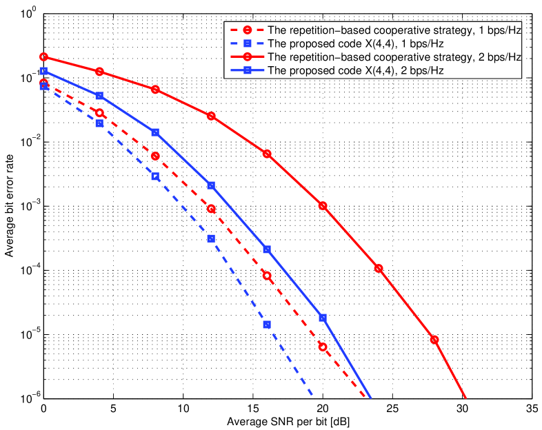
Figure 2: Comparison of the DOSTBCs/row-monomial DOSTBCs with the repetition-based cooperative strategy, $N=4$, $K=4$.

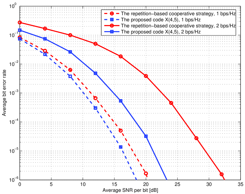
Figure 3: Comparison of the DOSTBCs/row-monomial DOSTBCs with the repetition-based cooperative strategy, $N=4$, $K=5$.

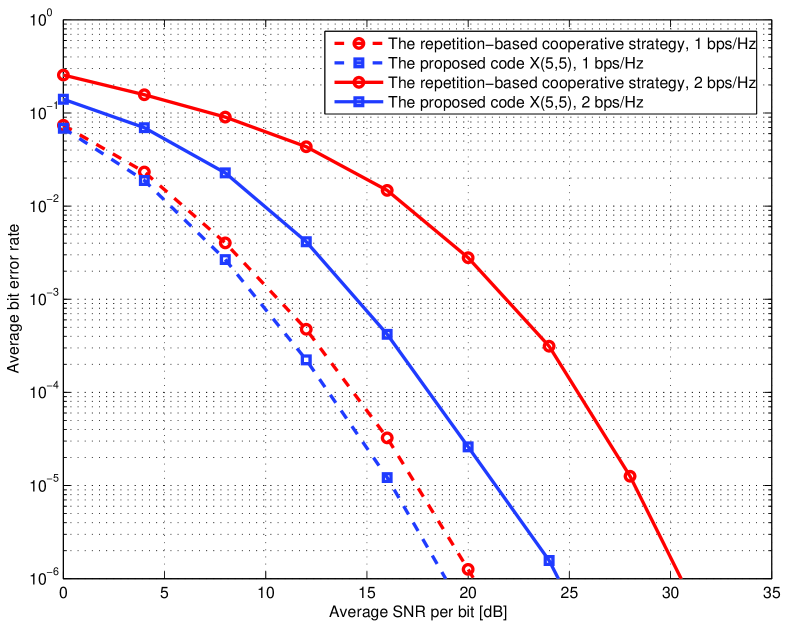
Figure 4: Comparison of the DOSTBCs/row-monomial DOSTBCs with the repetition-based cooperative strategy, $N=5$, $K=5$.

The comparison results are given in Figs. 2–4. It can be seen that the performance of the DOSTBCs is better than that of the repetition-based cooperative strategy in the whole Signal to Noise Ratio (SNR) range. The performance gain of the DOSTBCs is more impressive when the bandwidth efficiency is $2$ bps/Hz. For example, when $N=4$ and $K=4$, the performance gain of the DOSTBCs is approximately $7$ dB at $10^{-6}$ Bit Error Rate (BER). This is because the DOSTBCs have higher data-rate than the repetition-based cooperative strategy, and hence, they can use the modulation schemes with smaller constellation size to achieve the bandwidth efficiency $2$ bps/Hz. When the transmission power is fixed, smaller constellation size means larger minimum distance between the constellation points. Since the BER curves shift left when the minimum distance gets larger, the performance superiority of the DOSTBCs over the repetition-based cooperative strategy becomes more obvious when the bandwidth efficiency gets higher. Furthermore, because the BER curves of the DOSTBCs are parallel with those of the repetition-based cooperative strategy, they should have the same diversity order. It is well-known that the repetition-based cooperative strategy can achieve the full diversity order $K$. Therefore, the DOSTBCs also achieve the full diversity order $K$.

VII Conclusion

This paper focuses on designing high data-rate distributed space-time codes with single-symbol ML decodability and full diversity order. We propose a new type of distributed space-time codes, DOSTBCs, which are single-symbol decodable and have the full diversity order $K$. By deriving an upper bound of the data-rate of the DOSTBC, we show that the DOSTBCs have much better bandwidth efficiency than the widely used repetition-based cooperative strategy. However, the DOSTBCs achieving the upper bound of the data-rate are only found when $N$ and $K$ are both even. Then, further investigation is given to the row-monomial DOSTBCs, which result in diagonal noise covariance matrices at the destination terminal. The upper bound of the data-rate of the row-monomial DOSTBC is derived and it is equal to or slightly smaller than that of the DOSTBC. However, systematic construction methods of the row-monomial DOSTBCs achieving the upper bound of the data-rate are found for any values of $N$ and $K$. Lastly, the full diversity order of the DOSTBCs is justified by numerical results.

Appendix A

Proof of Lemma 1

The first condition is directly from the fact that the entries of $X$ are 0, $\pm h_{k}s_{n}$, $\pm h_{k}^{*}s_{n}^{*}$, or multiples of these indeterminates by j.

The proof of the second condition is by contradiction. We assume that $\mbox{\boldmath$A$}_{k}$ and $\mbox{\boldmath$B$}_{k}$ have non-zero entries at the same position, for example $[\mbox{\boldmath$A$}_{k}]_{n,t}$ and $[\mbox{\boldmath$B$}_{k}]_{n,t}$ are both non-zero. Then, $[\mbox{\boldmath$X$}]_{k,t}$ will be a linear combination of $h_{k}s_{n}$ and $h_{k}^{*}s_{n}^{*}$, which violates the definition of the DOSTBCs in Definition 1. Thus, $\mbox{\boldmath$A$}_{k}$ and $\mbox{\boldmath$B$}_{k}$ can not have non-zero entries at the same position.

The proof of the third condition is also by contradiction. In order to prove $\mbox{\boldmath$A$}_{k}$ is column-monomial, we assume that the $t$-th, $1\leq t\leq T$, column of it has two non-zero entries: $[\mbox{\boldmath$A$}_{k}]_{n_{1},t}$ and $[\mbox{\boldmath$A$}_{k}]_{n_{2},t}$, $n_{1}\neq n_{2}$. Then $[\mbox{\boldmath$X$}]_{k,t}$ will be a linear combination of $h_{k}s_{n_{1}}$ and $h_{k}s_{n_{2}}$, which violates the definition of the DOSTBCs in Definition 1. Therefore, any column of $\mbox{\boldmath$A$}_{k}$ can not contain two non-zero entries. In the same way, it can be easily shown that any column of $\mbox{\boldmath$A$}_{k}$ can not contain more than two non-zero entries, and hence, $\mbox{\boldmath$A$}_{k}$ is column-monomial. Similarly, we can show that $\mbox{\boldmath$B$}_{k}$ is column-monomial.

In order to prove $\mbox{\boldmath$A$}_{k}+\mbox{\boldmath$B$}_{k}$ is column-monomial, we assume that the $t$-th, $1\leq t\leq T$, column of it contains two non-zero entries: $[\mbox{\boldmath$A$}_{k}+\mbox{\boldmath$B$}_{k}]_{n_{1},t}$ and $[\mbox{\boldmath$A$}_{k}+\mbox{\boldmath$B$}_{k}]_{n_{2},t}$, $n_{1}\neq n_{2}$. Because we have already shown that $\mbox{\boldmath$A$}_{k}$ and $\mbox{\boldmath$B$}_{k}$ can not have non-zero entries at the same position, there are only two possibilities to make the assumption hold: 1) $[\mbox{\boldmath$A$}_{k}]_{n_{1},t}$ and $[\mbox{\boldmath$B$}_{k}]_{n_{2},t}$ are non-zero; 2) $[\mbox{\boldmath$A$}_{k}]_{n_{2},t}$ and $[\mbox{\boldmath$B$}_{k}]_{n_{1},t}$ are non-zero. Under the first possibility, $[\mbox{\boldmath$X$}]_{k,t}$ will be a linear combination of $h_{k}s_{n_{1}}$ and $h_{k}^{*}s_{n_{2}}^{*}$; under the second possibility, $[\mbox{\boldmath$X$}]_{k,t}$ will be a linear combination of $h_{k}s_{n_{2}}$ and $h_{k}^{*}s_{n_{1}}^{*}$. Since both of them violate the definition of the DOSTBCs in Definition 1, we can conclude that any column of $\mbox{\boldmath$A$}_{k}+\mbox{\boldmath$B$}_{k}$ can not contain two non-zero entries. In the same way, it can be easily shown that any column of $\mbox{\boldmath$A$}_{k}+\mbox{\boldmath$B$}_{k}$ can not contain more than two non-zero entries, and hence, $\mbox{\boldmath$A$}_{k}+\mbox{\boldmath$B$}_{k}$ is column-monomial.

Appendix B

Proof of Lemma 2

The sufficient part is easy to verify. We only prove the necessary part here, i.e. if (10) holds, $\mbox{\boldmath$A$}_{k}$ and $\mbox{\boldmath$B$}_{k}$ satisfy (12)–(16). When $k_{1}\neq k_{2}$, according to (10) and (11), $[\mbox{\boldmath$X$}\mbox{\boldmath$R$}^{-1}\mbox{\boldmath$X$}]_{k_{1},k_{2}}$ is given by

$$[\mbox{\boldmath$X$}\mbox{\boldmath$R$}^{-1}\mbox{\boldmath$X$}]_{k_{1},k_{2}} = h_{k_{1}}h_{k_{2}}^{*}\mbox{\boldmath$s$}\mbox{\boldmath$A$}_{k_{1}}\mbox{\boldmath$R$}^{-1}\mbox{\boldmath$A$}_{k_{2}}^{H}\mbox{\boldmath$s$}^{H}+h_{k_{1}}^{*}h_{k_{2}}^{*}\mbox{\boldmath$s$}^{*}\mbox{\boldmath$B$}_{k_{1}}\mbox{\boldmath$R$}^{-1}\mbox{\boldmath$A$}_{k_{2}}^{H}\mbox{\boldmath$s$}^{H}$$ (B.1)

$$+h_{k_{1}}h_{k_{2}}\mbox{\boldmath$s$}\mbox{\boldmath$A$}_{k_{1}}\mbox{\boldmath$R$}^{-1}\mbox{\boldmath$B$}_{k_{2}}^{H}\mbox{\boldmath$s$}^{T}+h_{k_{1}}^{*}h_{k_{2}}\mbox{\boldmath$s$}^{*}\mbox{\boldmath$B$}_{k_{1}}\mbox{\boldmath$R$}^{-1}\mbox{\boldmath$B$}_{k_{2}}^{H}\mbox{\boldmath$s$}^{T}$$

$$= 0.$$

Note that $h_{k_{1}}$ and $h_{k_{2}}$ can be any complex numbers. Thus, in order to make (B.1) hold for every possible value of $h_{k_{1}}$ and $h_{k_{2}}$, the following equalities must hold

$$\mbox{\boldmath$s$}\mbox{\boldmath$A$}_{k_{1}}\mbox{\boldmath$R$}^{-1}\mbox{\boldmath$A$}_{k_{2}}^{H}\mbox{\boldmath$s$}^{H} = 0$$ (B.2)

$$\mbox{\boldmath$s$}^{*}\mbox{\boldmath$B$}_{k_{1}}\mbox{\boldmath$R$}^{-1}\mbox{\boldmath$A$}_{k_{2}}^{H}\mbox{\boldmath$s$}^{H} = 0$$ (B.3)

$$\mbox{\boldmath$s$}\mbox{\boldmath$A$}_{k_{1}}\mbox{\boldmath$R$}^{-1}\mbox{\boldmath$B$}_{k_{2}}^{H}\mbox{\boldmath$s$}^{T} = 0$$ (B.4)

$$\mbox{\boldmath$s$}^{*}\mbox{\boldmath$B$}_{k_{1}}\mbox{\boldmath$R$}^{-1}\mbox{\boldmath$B$}_{k_{2}}^{H}\mbox{\boldmath$s$}^{T} = 0.$$ (B.5)

By using Lemma 1 of [24], we have (12), (13), and

$$\mbox{\boldmath$A$}_{k_{1}}\mbox{\boldmath$R$}^{-1}\mbox{\boldmath$B$}_{k_{2}}^{H}+\mbox{\boldmath$B$}_{k_{2}}^{*}\mbox{\boldmath$R$}^{-1}\mbox{\boldmath$A$}_{k_{1}}^{T} = \mbox{\boldmath$0$}_{N\times N},\hskip 56.9055pt1\leq k_{1}\neq k_{2}\leq K$$ (B.6)

$$\mbox{\boldmath$B$}_{k_{1}}\mbox{\boldmath$R$}^{-1}\mbox{\boldmath$A$}_{k_{2}}^{H}+\mbox{\boldmath$A$}_{k_{2}}^{*}\mbox{\boldmath$R$}^{-1}\mbox{\boldmath$B$}_{k_{1}}^{T} = \mbox{\boldmath$0$}_{N\times N},\hskip 56.9055pt1\leq k_{1}\neq k_{2}\leq K.$$ (B.7)

When $k_{1}=k_{2}=k$, according to (10) and (11), $[\mbox{\boldmath$X$}\mbox{\boldmath$R$}^{-1}\mbox{\boldmath$X$}]_{k,k}$ is given by

$$[\mbox{\boldmath$X$}\mbox{\boldmath$R$}^{-1}\mbox{\boldmath$X$}]_{k,k} = |h_{k}|^{2}\mbox{\boldmath$s$}(\mbox{\boldmath$A$}_{k}\mbox{\boldmath$R$}^{-1}\mbox{\boldmath$A$}_{k}^{H}+\mbox{\boldmath$B$}_{k}^{*}\mbox{\boldmath$R$}^{-1}\mbox{\boldmath$B$}_{k}^{T})\mbox{\boldmath$s$}^{H}$$ (B.8)

$$+h_{k}^{*}h_{k}^{*}\mbox{\boldmath$s$}^{*}\mbox{\boldmath$B$}_{k}\mbox{\boldmath$R$}^{-1}\mbox{\boldmath$A$}_{k}^{H}\mbox{\boldmath$s$}^{H}+h_{k}h_{k}\mbox{\boldmath$s$}\mbox{\boldmath$A$}_{k_{1}}\mbox{\boldmath$R$}^{-1}\mbox{\boldmath$B$}_{k}^{H}\mbox{\boldmath$s$}^{T}$$

$$= |h_{k}|^{2}\mbox{\boldmath$s$}\ {\mathrm{diag}}[D_{1,k},\cdots,D_{N,k}]\mbox{\boldmath$s$}^{H}.$$

For the same reason as in (B.1), the following equalities must hold

$$\mbox{\boldmath$s$}(\mbox{\boldmath$A$}_{k}\mbox{\boldmath$R$}^{-1}\mbox{\boldmath$A$}_{k}^{H}+\mbox{\boldmath$B$}_{k}^{*}\mbox{\boldmath$R$}^{-1}\mbox{\boldmath$B$}_{k}^{T})\mbox{\boldmath$s$}^{H} = \mbox{\boldmath$s$}\ {\mathrm{diag}}[D_{1,k},\cdots,D_{N,k}]\mbox{\boldmath$s$}^{H}$$ (B.9)

$$\mbox{\boldmath$s$}^{*}\mbox{\boldmath$B$}_{k}\mbox{\boldmath$R$}^{-1}\mbox{\boldmath$A$}_{k}^{H}\mbox{\boldmath$s$}^{H} = 0$$ (B.10)

$$\mbox{\boldmath$s$}\mbox{\boldmath$A$}_{k_{1}}\mbox{\boldmath$R$}^{-1}\mbox{\boldmath$B$}_{k}^{H}\mbox{\boldmath$s$}^{T} = 0.$$ (B.11)

By using Lemma 1 of [24] again, we have (16) and

$$\mbox{\boldmath$A$}_{k}\mbox{\boldmath$R$}^{-1}\mbox{\boldmath$B$}_{k}^{H}+\mbox{\boldmath$B$}_{k}^{*}\mbox{\boldmath$R$}^{-1}\mbox{\boldmath$A$}_{k}^{T} = \mbox{\boldmath$0$}_{N\times N},\hskip 56.9055pt1\leq k\leq K$$ (B.12)

$$\mbox{\boldmath$B$}_{k}\mbox{\boldmath$R$}^{-1}\mbox{\boldmath$A$}_{k}^{H}+\mbox{\boldmath$A$}_{k}^{*}\mbox{\boldmath$R$}^{-1}\mbox{\boldmath$B$}_{k}^{T} = \mbox{\boldmath$0$}_{N\times N},\hskip 56.9055pt1\leq k\leq K.$$ (B.13)

Combining (B.6) and (B.7) with (B.12) and (B.13), respectively, we have (14) and (15). This completes the proof of the necessary part.

Appendix C

Proof of Theorem 1

If a DOSTBC $X$ exists, (10) holds by Definition 1, and hence, (12)–(16) hold by Lemma 2. On the other hand, following the same way of the proof of Lemma 2, it can be easily shown that (17) holds if and only if

$$\mbox{\boldmath$A$}_{k_{1}}\mbox{\boldmath$A$}_{k_{2}}^{H} = \mbox{\boldmath$0$}_{N\times N},\hskip 56.9055pt1\leq k_{1}\neq k_{2}\leq K$$ (C.1)

$$\mbox{\boldmath$B$}_{k_{1}}\mbox{\boldmath$B$}_{k_{2}}^{H} = \mbox{\boldmath$0$}_{N\times N},\hskip 56.9055pt1\leq k_{1}\neq k_{2}\leq K$$ (C.2)

$$\mbox{\boldmath$A$}_{k_{1}}\mbox{\boldmath$B$}_{k_{2}}^{H}+\mbox{\boldmath$B$}_{k_{2}}^{*}\mbox{\boldmath$A$}_{k_{1}}^{T} = \mbox{\boldmath$0$}_{N\times N},\hskip 56.9055pt1\leq k_{1},k_{2}\leq K$$ (C.3)

$$\mbox{\boldmath$B$}_{k_{1}}\mbox{\boldmath$A$}_{k_{2}}^{H}+\mbox{\boldmath$A$}_{k_{2}}^{*}\mbox{\boldmath$B$}_{k_{1}}^{T} = \mbox{\boldmath$0$}_{N\times N},\hskip 56.9055pt1\leq k_{1},k_{2}\leq K$$ (C.4)

$$\mbox{\boldmath$A$}_{k}\mbox{\boldmath$A$}_{k}^{H}+\mbox{\boldmath$B$}^{*}_{k}\mbox{\boldmath$B$}^{T}_{k} = {\mathrm{diag}}[E_{1,k},\cdots,E_{N,k}],\hskip 56.9055pt1\leq k\leq K.$$ (C.5)

Therefore, in order to prove Theorem 1, we only need to show that, if (12)–(16) hold, (C.1)–(C.5) hold and $E_{n,k}$ is strictly positive.

First, we evaluate $[\mbox{\boldmath$R$}]_{t_{1},t_{2}}$. According to (8), when $t_{1}\neq t_{2}$, $[\mbox{\boldmath$R$}]_{t_{1},t_{2}}$ can be either null or a sum of several terms containing $|\rho f_{k}|^{2}$; when $t_{1}=t_{2}=t$, $[\mbox{\boldmath$R$}]_{t,t}$ is a sum of a constant 1, which is from the identity matrix, and several terms containing $|\rho f_{k}|^{2}$. Therefore, we can rewrite $[\mbox{\boldmath$R$}]_{t,t}$ as $[\mbox{\boldmath$R$}]_{t,t}=\bar{R}_{t,t}+1$, where $\bar{R}_{t,t}$ accounts for all the terms containing $|\rho f_{k}|^{2}$. $[\mbox{\boldmath$R$}^{-1}]_{t_{1},t_{2}}$ is given by $[\mbox{\boldmath$R$}^{-1}]_{t_{1},t_{2}}=C_{t_{2},t_{1}}/\mathrm{det}(\mbox{\boldmath$R$})$, where $C_{t_{2},t_{1}}$ is the matrix cofactor of $[\mbox{\boldmath$R$}]_{t_{2},t_{1}}$. When $t_{1}=t_{2}=t$, by the definition of matrix cofactor, $C_{t,t}$ contains a constant 1 generated by the product $\prod_{i=1,i\neq t}^{T}[\mbox{\boldmath$R$}]_{i,i}=\prod_{i=1,i\neq t}^{T}(\bar{R}_{i,i}+1)$. Furthermore, it is easy to see that the constant 1 is the only constant term in $C_{t,t}$. Thus, $C_{t,t}$ can be rewritten as $C_{t,t}=\bar{C}_{t,t}+1$, where no constant term is in $\bar{C}_{t,t}$. Consequently, $[\mbox{\boldmath$R$}^{-1}]_{t,t}$ can be rewritten as $[\mbox{\boldmath$R$}^{-1}]_{t,t}=\bar{C}_{t,t}/\mathrm{det}(\mbox{\boldmath$R$})+1/\mathrm{det}(\mbox{\boldmath$R$})$. When $t_{1}\neq t_{2}$, $C_{t_{2},t_{1}}$ does not contain any constant term, and hence, $[\mbox{\boldmath$R$}^{-1}]_{t_{1},t_{2}}$ does not contain the term $1/\mathrm{det}(\mbox{\boldmath$R$})$. Therefore, we can extract the term $1/\mathrm{det}(\mbox{\boldmath$R$})$ from every main diagonal entry of $\mbox{\boldmath$R$}^{-1}$ and rewrite $\mbox{\boldmath$R$}^{-1}$ in the following way

$$\mbox{\boldmath$R$}^{-1} = \frac{1}{\mathrm{det}(\mbox{\boldmath$R$})}\bar{\mbox{\boldmath$C$}}+\frac{1}{\mathrm{det}(\mbox{\boldmath$R$})}\mbox{\boldmath$I$}_{T\times T}.$$ (C.6)

Then we show that (C.1) holds if (12) holds. If (12) holds, we have

$$\mbox{\boldmath$A$}_{k_{1}}\mbox{\boldmath$R$}^{-1}\mbox{\boldmath$A$}_{k_{2}}^{H}=\frac{1}{\mathrm{det}(\mbox{\boldmath$R$})}\mbox{\boldmath$A$}_{k_{1}}\bar{\mbox{\boldmath$C$}}\mbox{\boldmath$A$}_{k_{2}}^{H}+\frac{1}{\mathrm{det}(\mbox{\boldmath$R$})}\mbox{\boldmath$A$}_{k_{1}}\mbox{\boldmath$A$}_{k_{2}}^{H}=\mbox{\boldmath$0$}_{N\times N}.$$ (C.7)

Note that $\mbox{\boldmath$R$}^{-1}$ and $\bar{\mbox{\boldmath$C$}}$ are random matrices. In order to make (C.7) hold for every possible $\mbox{\boldmath$R$}^{-1}$ and $\bar{\mbox{\boldmath$C$}}$, both terms in (C.7) must be equal to zero. Therefore, (C.1) holds. Similarly, we can show that (C.2)–(C.4) hold if (13)–(15) hold. Now, we show that (C.5) holds if (16) holds. If (16) holds, we have

$$\mbox{\boldmath$A$}_{k}\mbox{\boldmath$R$}^{-1}\mbox{\boldmath$A$}_{k}^{H}+\mbox{\boldmath$B$}^{*}_{k}\mbox{\boldmath$R$}^{-1}\mbox{\boldmath$B$}^{T}_{k} = \frac{1}{\mathrm{det}(\mbox{\boldmath$R$})}\left(\mbox{\boldmath$A$}_{k}\bar{\mbox{\boldmath$C$}}\mbox{\boldmath$A$}_{k}^{H}+\mbox{\boldmath$B$}^{*}_{k}\bar{\mbox{\boldmath$C$}}\mbox{\boldmath$B$}^{T}_{k}\right)+\frac{1}{\mathrm{det}(\mbox{\boldmath$R$})}\left(\mbox{\boldmath$A$}_{k}\mbox{\boldmath$A$}_{k}^{H}+\mbox{\boldmath$B$}^{*}_{k}\mbox{\boldmath$B$}^{T}_{k}\right)$$ (C.8)

$$= {\mathrm{diag}}[D_{1,k},\cdots,D_{N,k}].$$

For the same reason as in (C.7), the off-diagonal entries of $\mbox{\boldmath$A$}_{k}\mbox{\boldmath$A$}_{k}^{H}+\mbox{\boldmath$B$}^{*}_{k}\mbox{\boldmath$B$}^{T}_{k}$ must be zero, and hence, (C.5) holds.

Lastly, we show that $E_{n,k}$ is strictly positive if (16) holds. From (16) and (C.5), we have

$$D_{n,k} = \sum_{t=1}^{T}\sum_{i=1}^{T}[\mbox{\boldmath$R$}^{-1}]_{i,t}([\mbox{\boldmath$A$}_{k}]_{n,i}[\mbox{\boldmath$A$}_{k}]_{n,t}^{*}+[\mbox{\boldmath$B$}_{k}]_{n,i}^{*}[\mbox{\boldmath$B$}_{k}]_{n,t})$$ (C.9)

$$E_{n,k} = \sum_{t=1}^{T}(|[\mbox{\boldmath$A$}_{k}]_{n,t}|^{2}+|[\mbox{\boldmath$B$}_{k}]_{n,t}|^{2}).$$ (C.10)

Since $D_{n,k}$ is non-zero, at least one $[\mbox{\boldmath$A$}_{k}]_{n,t}$ or one $[\mbox{\boldmath$B$}_{k}]_{n,t}$ is non-zero. Furthermore, the modulus of that non-zero entry is 1 by Lemma 1. Therefore, $E_{n,k}=\sum_{t=1}^{T}(|[\mbox{\boldmath$A$}_{k}]_{n,t}|^{2}+|[\mbox{\boldmath$B$}_{k}]_{n,t}|^{2})\geq 1$ is strictly positive, which completes the proof of Theorem 1.

Appendix D

Proof of Theorem 2

Let $\underline{\mbox{\boldmath$A$}}=[\mbox{\boldmath$A$}_{1},\cdots,\mbox{\boldmath$A$}_{K}]^{T}$ and $\underline{\mbox{\boldmath$B$}}=[\mbox{\boldmath$B$}_{1},\cdots,\mbox{\boldmath$B$}_{K}]^{T}$; then the dimension of $\underline{\mbox{\boldmath$A$}}$ and $\underline{\mbox{\boldmath$B$}}$ is $NK\times T$. From (C.1), every row of $\mbox{\boldmath$A$}_{k_{1}}$ is orthogonal with every row of $\mbox{\boldmath$A$}_{k_{2}}$ when $k_{1}\neq k_{2}$. Furthermore, because $\mbox{\boldmath$A$}_{k}$ is column-monomial by Lemma 1, every row of $\mbox{\boldmath$A$}_{k}$ is orthogonal with every other row of $\mbox{\boldmath$A$}_{k}$. Therefore, any two different rows in $\underline{\mbox{\boldmath$A$}}$ are orthogonal with each other, and hence, ${\mathrm{rank}}(\underline{\mbox{\boldmath$A$}})=\sum_{k=1}^{K}{\mathrm{rank}}(\mbox{\boldmath$A$}_{k})$. Similarly, any two different rows in $\underline{\mbox{\boldmath$B$}}$ are orthogonal with each other, and hence, ${\mathrm{rank}}(\underline{\mbox{\boldmath$B$}})=\sum_{k=1}^{K}{\mathrm{rank}}(\mbox{\boldmath$B$}_{k})$.

On the other hand, by (C.5), we have

$${\mathrm{rank}}(\mbox{\boldmath$A$}_{k})+{\mathrm{rank}}(\mbox{\boldmath$B$}_{k})\geq{\mathrm{rank}}({\mathrm{diag}}[E_{1,k},\cdots,E_{N,k}])=N,$$ (D.1)

where the inequality is from the rank inequality 3) in [23], and hence,

$$\sum_{k=1}^{K}{\mathrm{rank}}(\mbox{\boldmath$A$}_{k})+\sum_{k=1}^{K}{\mathrm{rank}}(\mbox{\boldmath$B$}_{k})\geq NK.$$ (D.2)

Because ${\mathrm{rank}}(\underline{\mbox{\boldmath$A$}})$ and ${\mathrm{rank}}(\underline{\mbox{\boldmath$B$}})$ are integers, we have

$${\mathrm{rank}}(\underline{\mbox{\boldmath$A$}})=\sum_{k=1}^{K}{\mathrm{rank}}(\mbox{\boldmath$A$}_{k})\geq\left\lceil\frac{NK}{2}\right\rceil$$ (D.3)

or

$${\mathrm{rank}}(\underline{\mbox{\boldmath$B$}})=\sum_{k=1}^{K}{\mathrm{rank}}(\mbox{\boldmath$B$}_{k})\geq\left\lceil\frac{NK}{2}\right\rceil.$$ (D.4)

If (D.3) is true, $T\geq{\mathrm{rank}}(\underline{\mbox{\boldmath$A$}})\geq\left\lceil(NK)/2\right\rceil$ and (19) holds. If (D.4) is true, the same conclusion can be made.

Appendix E

Proof of Theorem 3

The sufficient part is easy to verify. We only prove the necessary part here, i.e. if $R$ is a diagonal matrix, $\mbox{\boldmath$A$}_{k}$ and $\mbox{\boldmath$B$}_{k}$ are row-monomial. This is done by contradiction. If $R$ is a diagonal matrix, the off-diagonal entries $[\mbox{\boldmath$R$}]_{t_{1},t_{2}}$, $1\leq t_{1}\neq t_{2}\leq T$, are equal to 0. According to (8), we have

$$[\mbox{\boldmath$R$}]_{t_{1},t_{2}}=\sum_{k=1}^{K}\left[|\rho f_{k}|^{2}\left(\sum_{n=1}^{N}[\mbox{\boldmath$A$}_{k}]_{n,t_{1}}^{*}[\mbox{\boldmath$A$}_{k}]_{n,t_{2}}+\sum_{n=1}^{N}[\mbox{\boldmath$B$}_{k}]_{n,t_{1}}^{*}[\mbox{\boldmath$B$}_{k}]_{n,t_{2}}\right)\right]=0.$$ (E.1)

In order to make the equality hold for every possible $f_{k}$, the following equality must hold

$$\sum_{n=1}^{N}[\mbox{\boldmath$A$}_{k}]_{n,t_{1}}^{*}[\mbox{\boldmath$A$}_{k}]_{n,t_{2}}+\sum_{n=1}^{N}[\mbox{\boldmath$B$}_{k}]_{n,t_{1}}^{*}[\mbox{\boldmath$B$}_{k}]_{n,t_{2}} = 0,\hskip 42.67912pt1\leq k\leq K.$$ (E.2)

Let us assume that the $n^{{}^{\prime}}$-th, $1\leq n^{{}^{\prime}}\leq N$, row of $\mbox{\boldmath$A$}_{k}$ contains two non-zero entries: $[\mbox{\boldmath$A$}_{k}]_{n^{{}^{\prime}},t_{1}}$ and $[\mbox{\boldmath$A$}_{k}]_{n^{{}^{\prime}},t_{2}}$, $1\leq t_{1}\neq t_{2}\leq T$. Because $\mbox{\boldmath$A$}_{k}$ is column-monomial according to Lemma 1, $[\mbox{\boldmath$A$}_{k}]_{n,t_{1}}=[\mbox{\boldmath$A$}_{k}]_{n,t_{2}}=0$, $1\leq n\neq n^{{}^{\prime}}\leq N$, and hance,

$$\sum_{n=1}^{N}[\mbox{\boldmath$A$}_{k}]_{n,t_{1}}^{*}[\mbox{\boldmath$A$}_{k}]_{n,t_{2}}=[\mbox{\boldmath$A$}_{k}]_{n^{{}^{\prime}},t_{1}}^{*}[\mbox{\boldmath$A$}_{k}]_{n^{{}^{\prime}},t_{2}}\neq 0.$$ (E.3)

On the other hand, because $\mbox{\boldmath$A$}_{k}$ and $\mbox{\boldmath$B$}_{k}$ can not have non-zero entries at the same place according to Lemma 1, we have $[\mbox{\boldmath$B$}_{k}]_{n^{{}^{\prime}},t_{1}}=[\mbox{\boldmath$B$}_{k}]_{n^{{}^{\prime}},t_{2}}=0$. Furthermore, because $\mbox{\boldmath$A$}_{k}+\mbox{\boldmath$B$}_{k}$ is column-monomial, $[\mbox{\boldmath$B$}_{k}]_{n,t_{1}}=[\mbox{\boldmath$B$}_{k}]_{n,t_{2}}=0$, $1\leq n\neq n^{{}^{\prime}}\leq N$. Therefore, $[\mbox{\boldmath$B$}_{k}]_{n,t_{1}}=[\mbox{\boldmath$B$}_{k}]_{n,t_{2}}=0$, $1\leq n\leq N$, and consequently, $\sum_{n=1}^{N}[\mbox{\boldmath$B$}_{k}]_{n,t_{1}}^{*}[\mbox{\boldmath$B$}_{k}]_{n,t_{2}}=0$. It follows from (E.2) and $\sum_{n=1}^{N}[\mbox{\boldmath$B$}_{k}]_{n,t_{1}}^{*}[\mbox{\boldmath$B$}_{k}]_{n,t_{2}}=0$ that

$$\sum_{n=1}^{N}[\mbox{\boldmath$A$}_{k}]_{n,t_{1}}^{*}[\mbox{\boldmath$A$}_{k}]_{n,t_{2}}=0.$$ (E.4)

Because (E.3) and (E.4) contradict with each other, we can conclude that any row of $\mbox{\boldmath$A$}_{k}$ can not contain two non-zero entries. Furthermore, in the same way, it can be easily shown that any row of $\mbox{\boldmath$A$}_{k}$ can not contain more than two non-zero entries, and hence, $\mbox{\boldmath$A$}_{k}$ is row-monomial. Similarly, we can show that $\mbox{\boldmath$B$}_{k}$ is row-monomial, which completes the proof of the necessary part.

Appendix F

Proof of Lemma 3

The proof is by contradiction. We assume that the $t^{{}^{\prime}}$-th column of $\mbox{\boldmath$A$}_{k_{1}}$ and $\mbox{\boldmath$A$}_{k_{2}}$, $1\leq k_{1}\neq k_{2}\leq K$, contains a non-zero entry $[\mbox{\boldmath$A$}_{k_{1}}]_{n_{1},t^{{}^{\prime}}}$ and a non-zero entry $[\mbox{\boldmath$A$}_{k_{2}}]_{n_{2},t^{{}^{\prime}}}$, respectively. By Definition 2, $\mbox{\boldmath$A$}_{k_{1}}$ and $\mbox{\boldmath$A$}_{k_{2}}$ are both row-monomial, we have $[\mbox{\boldmath$A$}_{k_{1}}]_{n_{1},t}=[\mbox{\boldmath$A$}_{k_{2}}]_{n_{2},t}=0$, $1\leq t\neq t^{{}^{\prime}}\leq T$, and hence,

$$\sum_{t=1}^{T}[\mbox{\boldmath$A$}_{k_{1}}]_{n_{1},t}[\mbox{\boldmath$A$}_{k_{2}}]_{n_{2},t}^{*}=[\mbox{\boldmath$A$}_{k_{1}}]_{n_{1},t^{{}^{\prime}}}[\mbox{\boldmath$A$}_{k_{2}}]_{n_{2},t^{{}^{\prime}}}^{*}\neq 0.$$ (F.1)

On the other hand, from (C.1), $[\mbox{\boldmath$A$}_{k_{1}}\mbox{\boldmath$A$}_{k_{2}}^{H}]_{n_{1},n_{2}}$ is given by

$$[\mbox{\boldmath$A$}_{k_{1}}\mbox{\boldmath$A$}_{k_{2}}^{H}]_{n_{1},n_{2}}=\sum_{t=1}^{T}[\mbox{\boldmath$A$}_{k_{1}}]_{n_{1},t}[\mbox{\boldmath$A$}_{k_{2}}]_{n_{2},t}^{*}=0.$$ (F.2)

Because (F.1) and (F.2) contradict with each other, we conclude that $\mbox{\boldmath$A$}_{k_{1}}$ and $\mbox{\boldmath$A$}_{k_{2}}$, $1\leq k_{1}\neq k_{2}\leq K$, can not contain non-zero entries on the same column simultaneously. Therefore, $\mbox{\boldmath$A$}_{k_{1}}$ and $\mbox{\boldmath$A$}_{k_{2}}$ are column-disjoint when $k_{1}\neq k_{2}$. Similarly, we can show that $\mbox{\boldmath$B$}_{k_{1}}$ and $\mbox{\boldmath$B$}_{k_{2}}$ are column-disjoint when $k_{1}\neq k_{2}$.

Appendix G

Proof of Lemma 4

If no Type-II column exists in $X$, it is trivial that the number of the Type-II columns in $X$ is even. If there is one Type-II column in $X$, without loss of generality, we assume that the $t_{1}$-th column in $X$ is a Type-II column and it contains $h_{k_{1}}s_{n_{1}}$ and $h_{k_{2}}^{*}s_{n_{2}}^{*}$ on the $k_{1}$-th and $k_{2}$-th row, respectively. Consequently, the inner product of the $k_{1}$-th row and the $k_{2}$-th row will contain the term $h_{k_{1}}s_{n_{1}}h_{k_{2}}s_{n_{2}}$. Because $X$ is a row-monomial DOSTBC, the inner product of any two different rows is null by (17). Hence, the inner product of the $k_{1}$-th row and the $k_{2}$-th row should contain the term $-h_{k_{1}}s_{n_{1}}h_{k_{2}}s_{n_{2}}$ as well to cancel the term $h_{k_{1}}s_{n_{1}}h_{k_{2}}s_{n_{2}}$. Thus, there must be another Type-II column, for example the $t_{2}$-th column, $t_{1}\neq t_{2}$, which contains $-h_{k_{1}}s_{n_{2}}$ and $h_{k_{2}}^{*}s_{n_{1}}^{*}$ on the $k_{1}$-th and $k_{2}$-th row, respectively. Therefore, the Type-II columns in $X$ always appear in pairs, and hence, the total number of the Type-II columns in $X$ is even.

For convenience, we will refer to any entry in $X$ that contains $s_{n}$ or $s_{n}^{*}$ as the $s_{n}$-entry. If no $s_{n}$-entry exists in the Type-II columns of $X$, it is trivial that the total number of $s_{n}$-entries in the Type-II columns of $X$ is even. If there is one $s_{n}$-entry in a Type-II column of $X$, we assume it contains $s_{n}$ without loss of generality. From the proof of the first property in Lemma 4, we can see that there must be an $s_{n}$-entry in another Type-II column and it contains $s_{n}^{*}$. Therefore, in the Type-II columns of $X$, the $s_{n}$-entries always appear in pairs, and hence, the total number of the $s_{n}$-entries in the Type-II columns of $X$ is even.

Appendix H

Proof of Theorem 4

For convenience, we will refer to any entry in $X$ that contains $s_{n}$ or $s_{n}^{*}$ as the $s_{n}$-entry. Let $U$ denote the total number of non-zero entries in $X$; $V_{n}$ the total number of $s_{n}$-entries in $X$; $W_{k}$ the total number of non-zero entries in the $k$-th row of $X$. Obviously, $U=\sum_{n=1}^{N}V_{n}=\sum_{k=1}^{K}W_{k}$. According to (C.5) and (C.10), at least one $[\mbox{\boldmath$A$}_{k}]_{n,t}$ or one $[\mbox{\boldmath$B$}_{k}]_{n,t}$ is non-zero, $1\leq n\leq N$ and $1\leq k\leq K$. Thus, every row of $X$ has at least one $s_{n}$-entry, $1\leq n\leq N$. On the other hand, by the row-monomial condition of $\mbox{\boldmath$A$}_{k}$ and $\mbox{\boldmath$B$}_{k}$, every row of $X$ has at most two $s_{n}$-entries, where one contains $s_{n}$ and the other contains $s_{n}^{*}$. Therefore, every row of $X$ contains at least $N$ and at most $2N$ non-zero entries, i.e. $N\leq W_{k}\leq 2N$, $1\leq k\leq K$. For the same reason, we have $K\leq V_{n}\leq 2K$, $1\leq n\leq N$. Consequently, we have $NK\leq U\leq 2NK$.

Case I: $N=2l$ and $K=2m$. When $N=2l$ and $K=2m$, $U\geq NK=4lm$. Because a pair of Type-II columns contains 4 non-zero entries, at least $\left\lceil 4lm/4\right\rceil$ pairs of Type-II columns are needed to transmit all the non-zero entries. Since $T$ is the total number of columns in $X$, we have the following inequality

$$T\geq 2\left\lceil\frac{4lm}{4}\right\rceil=2lm,$$ (H.1)

and hence,

$${\mathrm{Rate}}_{r} \leq \frac{1}{m}.$$ (H.2)

Case II: $N=2l+1$ and $K=2m$. When $N=2l+1$ and $K=2m$, without loss of generality, we assume $W_{1},\cdots,W_{w}$ are even and $W_{1+w},\cdots,W_{2m}$ are odd, where $1\leq w\leq 2m$. We first have $U\geq NK=4lm+2m$. Furthermore, because $W_{k}$ is even for $1\leq k\leq w$, $W_{k}\geq N+1=2l+2$. Consequently, $U\geq 4lm+2m+w$. On the other hand, because the Type-II columns always appear in pairs, the $k$-th row of $X$, $w+1\leq k\leq 2m$, must contain at least one Type-I column; otherwise, $W_{k}$ will be even, which violates our assumption. Therefore, there are at least $2m-w$ Type-I columns in $X$ and they contain $2m-w$ non-zero entries. Because a pair of Type-II columns contains 4 non-zero entries, the rest non-zero entries need at least $\left\lceil(4lm+2m+w-(2m-w))/4\right\rceil$ pairs of Type-II columns to transmit. Therefore, we have the following inequality

$$T \geq 2m-w+2\left\lceil\frac{4lm+2m+w-(2m-w)}{4}\right\rceil$$ (H.3)

$$\geq 2m-w+\frac{4lm+2m+w-(2m-w)}{2}$$ (H.4)

$$= 2lm+2m,$$ (H.5)

and hence,

$${\mathrm{Rate}}_{r} \leq \frac{2l+1}{2lm+2m}.$$ (H.6)

Case III: $N=2l$ and $K=2m+1$. When $N=2l$ and $K=2m+1$, without loss of generality, we assume $V_{1},\cdots,V_{v}$ are even and $V_{v+1},\cdots,V_{2l}$ are odd, where $1\leq v\leq 2l$. We first have $U\geq NK=4lm+2l$. Furthermore, because $V_{n}$ is even for $1\leq n\leq v$, $V_{n}\geq K+1=2m+2$. Consequently, $U\geq 4lm+2l+v$. On the other hand, because the total number of $s_{n}$-entries in the Type-II columns of $X$ is even, at least one $s_{n}$-entry, $v+1\leq n\leq 2l$, is in a Type-I column; otherwise, $V_{n}$ will be even, which violates our assumption. Thus, there are at least $2l-v$ Type-I columns in $X$ and they contain $2l-v$ non-zero entries. Because a pair of Type-II columns contains 4 non-zero entries, the rest non-zero entries need at least $\left\lceil(4lm+2l+v-(2l-v))/4\right\rceil$ pairs of Type-II columns to transmit. Therefore, we have the following inequality

$$T \geq 2l-v+2\left\lceil\frac{4lm+2l+v-(2l-v)}{4}\right\rceil$$ (H.7)

$$\geq 2l-v+\frac{4lm+2l+v-(2l-v)}{2}$$ (H.8)

$$= 2lm+2l,$$ (H.9)

and hence,

$${\mathrm{Rate}}_{r} \leq \frac{1}{m+1}.$$ (H.10)

Case IV: $N=2l+1$ and $K=2m+1$. When $N=2l+1$ and $K=2m+1$, we can assume that $W_{1},\cdots,W_{w}$ are even and $W_{1+w},\cdots,W_{2m+1}$ are odd, where $1\leq w\leq 2m+1$. By following the proof of Case II, we have

$$T \geq 2m+1-w+2\left\lceil\frac{4lm+2l+2m+1+w-(2m+1-w)}{4}\right\rceil$$ (H.11)

$$\geq 2m+1-w+\frac{4lm+2l+2m+1+w-(2m+1-w)}{2}$$ (H.12)

$$= 2lm+2m+l+1.$$ (H.13)

On the other hand, we can assume $V_{1},\cdots,V_{v}$ are even and $V_{v+1},\cdots,V_{2l+1}$ are odd, where $1\leq v\leq 2l+1$. By following the proof of Case III, we have

$$T \geq 2l+1-v+2\left\lceil\frac{4lm+2l+2m+1+v-(2l+1-v)}{4}\right\rceil$$ (H.14)

$$\geq 2l+1-v+\frac{4lm+2l+2m+1+v-(2l+1-v)}{2}$$ (H.15)

$$= 2lm+2l+m+1.$$ (H.16)

From (H.13) and (H.16), it is immediate that

$$T \geq \max(2lm+2m+l+1,2lm+2l+m+1),$$ (H.17)

and

$${\mathrm{Rate}}_{r} \leq \min\left(\frac{2l+1}{2lm+2m+l+1},\frac{2l+1}{2lm+2l+m+1}\right).$$ (H.18)

TABLE I: Upper Bounds of the Data-Rates of the DOSTBC and Row-Monomial DOSTBC

	DOSTBCs	row-monomial DOSTBCs	difference
$N=2l$, $K=2m$	$\frac{1}{m}$	$\frac{1}{m}$	0
$N=2l+1$, $K=2m$	$\frac{1}{m}$	$\frac{2l+1}{2lm+2m}$	$\frac{1}{2lm+2m}$
$N=2l$, $K=2m+1$	$\frac{2}{2m+1}$	$\frac{1}{1+m}$	$\frac{1}{(2m+1)(m+1)}$
$N=2l+1$, $K=2m+1$	$\frac{2l+1}{2lm+l+m+1}$	$\min\left(\frac{2l+1}{2lm+2m+l+1}\right.,$	$\max\left(\frac{m(2l+1)}{(2lm+l+m+1)(2lm+2m+l+1)}\right.,$
		$\left.\frac{2l+1}{2lm+2l+m+1}\right)$	$\left.\frac{l(2l+1)}{(2lm+l+m+1)(2lm+2l+m+1)}\right)$

References

- [1] A. Sendonaris, E. Erkip, and B. Aazhang, “User cooperation diversity–Part I: System description,” IEEE Trans. Commun., vol. 51, pp. 1927–1938, Nov. 2003.
- [2] ——, “User cooperation diversity–Part II: Implementation aspects and performance analysis,” IEEE Trans. Commun., vol. 51, pp. 1939–1948, Nov. 2003.
- [3] J. N. Laneman, D. N. C. Tse, and G. W. Wornell, “Cooperative diversity in wireless networks: Efficient protocols and outage behavior,” IEEE Trans. Inform. Theory, vol. 50, pp. 3062–3080, Dec. 2004.
- [4] J. N. Laneman and G. W. Wornell, “Energy-efficient antenna sharing and relaying for wireless networks,” in Proc. of WCNC 2000, vol. 1, Sep. 2000, pp. 7–12.
- [5] Md. Z. A. Khan and B. S. Rajan, “Single-symbol maximum likelihood decodable linear STBCs,” IEEE Trans. Inform. Theory, vol. 52, pp. 2062–2091, May 2006.
- [6] P. A. Anghel and M. Kaveh, “Exact symbol error probability of a cooperative network in a rayleigh-fading environment,” IEEE Trans. Wireless Commun., vol. 3, pp. 1416–1421, Sep. 2004.
- [7] A. Ribeiro, X. Cai, and G. B. Giannakis, “Symbol error probabilities for general cooperative links,” IEEE Trans. Wireless Commun., vol. 4, pp. 1264–1273, May 2005.
- [8] M. O. Hasna and M. S. Alouini, “End-to-end performance of transmission systems with relays over rayleigh–fading channels,” IEEE Trans. Wireless Commun., vol. 2, pp. 1126–1131, Nov. 2003.
- [9] ——, “Harmonic mean and end-to-end performance of transmission systems with relays,” IEEE Trans. Commun., vol. 52, pp. 130–135, Jan. 2004.
- [10] D. Chen and J. N. Laneman, “Modulation and demodulation for cooperative diversity in wireless systems,” IEEE Trans. Wireless Commun., vol. 5, pp. 1785–1794, July 2006.
- [11] J. N. Laneman and G. W. Wornell, “Distributed space-time-coded protocols for exploiting cooperative diversity in wireless networks,” IEEE Trans. Inform. Theory, vol. 49, pp. 2415–2425, Oct. 2003.
- [12] R. U. Nabar, H. Bölcskei, and F. W. Kneubühler, “Fading relay channels: Performance limits and space-time signal designs,” IEEE J. Select. Areas Commun., vol. 22, pp. 1099–1109, Aug. 2004.
- [13] S. Yang and J.-C. Belfiore, “Optimal space-time codes for the MIMO amplify-and-forward cooperative channel,” IEEE Trans. Inform. Theory, submitted for publication, Sept. 2005.
- [14] H. El Gamal and D. Aktas, “Distributed space-time filtering for cooperative wireless networks,” in Proc. IEEE GLOBECOM’03, vol. 4, Dec. 2003, pp. 1826–1830.
- [15] S. Yiu, R. Schober, and L. Lampe, “Distributed space-time block coding,” IEEE Trans. Commun., vol. 54, pp. 1195–1206, July 2006.
- [16] Y. Li and X.-G. Xia, “A family of distributed space-time trellis codes with asynchronous cooperative diversity,” IEEE Trans. Commun., submitted for publication, Nov. 2004.
- [17] Y. Jing and B. Hassibi, “Distributed space-time coding in wireless relay networks–Part I: basic diversity results,” IEEE Trans. Wireless Commun., accepted for publication, July 2004.
- [18] Y. Jing and B. Hassibi, “Distributed space-time coding in wireless relay network–Part II: tighter upper bounds and a more general case,” IEEE Trans. Wireless Commun., accepted for publication, July 2004.
- [19] Y. Hua, Y. Mei, and Y. Cheng, “Wireless antennas-making wireless communications perform like wireline communications,” in Proc. IEEE AP-S Topical Conference on Wireless Communication Technology, Oct. 2003, pp. 47–73.
- [20] S. Alamouti, “A simple transmit diversity technique for wireless communications,” IEEE J. Select. Areas Commun., vol. 16, pp. 1451–1458, Aug. 1998.
- [21] V. Tarokh, H. Jafarkhani, and A. R. Calderbank, “Space-time block codes from orthogonal designs,” IEEE Trans. Inform. Theory, vol. 45, pp. 1456–1467, July 1999.
- [22] Y. Jing and H. Jafarkhani, “Using orthogonal and quasi-orthogonal designs in wireless relay networks,” IEEE GLOBECOM‘06, accepted for publication, Nov. 2006.
- [23] H. Wang and X.-G. Xia, “Upper bounds of rates of complex orthogonal space-time block codes,” IEEE Trans. Inform. Theory, vol. 49. pp. 2788–2796, Oct. 2003.
- [24] X.-B. Liang and X.-G. Xia, “On the nonexistence of rate-one generalized complex orthogonal designs,” IEEE Trans. Inform. Theory, vol. 49, pp. 2984–2989, Nov. 2003.
- [25] W. Su and X.-G. Xia, “Two generalized complex orthogonal space-time block codes of rates 7/11 and 3/5 for 5 and 6 transmit antennas,” IEEE Trans. Inform. Theory, vol. 49, pp. 313–316, Jan. 2003.
- [26] W. Su, X.-G. Xia, and K. J. R. Liu, “A systematic design of high-rate complex orthogonal space-time block codes,” IEEE Commun. Lett., vol. 8, pp. 380–382, June 2004.
- [27] H.-B. Kan and H. Shen, “A counterexample for the open problem on the minimal delays of orthogonal designs with maximal rates,” IEEE Trans. Inform. Theory, vol. 51, pp. 355–359, Jan. 2005.
- [28] X.-B. Liang, “Orthogonal designs with maximal rates,” IEEE Trans. Inform. Theory, vol. 49, pp. 2468–2503, Oct. 2003.