Set-Theoretic Preliminaries for Computer Scientists

Abstract

The basics of set theory are usually copied, directly or indirectly, by computer scientists from introductions to mathematical texts. Often mathematicians are content with special cases when the general case is of no mathematical interest. But sometimes what is of no mathematical interest is of great practical interest in computer science. For example, non-binary relations in mathematics tend to have numerical indexes and tend to be unsorted. In the theory and practice of relational databases both these simplifications are unwarranted. In response to this situation we present here an alternative to the “set-theoretic preliminaries” usually found in computer science texts. This paper separates binary relations from the kind of relations that are needed in relational databases. Its treatment of functions supports both computer science in general and the kind of relations needed in databases. As a sample application this paper shows how the mathematical theory of relations naturally leads to the relational data model and how the operations on relations are by themselves already a powerful vehicle for queries.

1 Introduction

Mathematics is more useful than computer scientists tend to think. I am not talking about specialized areas of computer science with strongly developed mathematical theories, like graph theory in computer networks or posets and lattices for programming language semantics. These are solid extensions of the traditional notion of Applied Mathematics.

No, I’m talking about the mundane mathematics that falls into the cracks between these well-developed areas: basic facts about sets, functions, and relations. I refer to the material that gets relegated to the desultory miscellanies added to texts under the name of “set-theoretic preliminaries”. The reason for the perfunctory way in which these are compiled is that computer scientists are ambivalent about basic set theory: they don’t care for that stuff, yet dare not omit it.

My own lack of understanding in this area resulted in difficulties with the relational model. Accordingly, I include it as a case study of how basic set theory could have clarified these difficulties, which are also found in the literature.

The ambivalence concerning the set-theoretic preliminaries is understandable. Is a proper treatment not going to lead to an unacceptably large mass of definitions and theorems? After all, set theory is nothing if it is not done rigorously. In other parts of mathematics you can start right away with what interests you and you refer to something else for the foundation. No such help is available when you deal with the foundation itself.

This paper is intended to improve this situation. My model is Halmos’s Naïve Set Theory [4], which shows that one can be precise enough and yet easily digestible without losing anything essential. Halmos’s book was aimed at normal mathematicians; that is, those who have no interest in set theory, yet cannot do without it. It is therefore ideal for computer scientists, who are in the same position. Though set theory is no different for mathematicians than it is for computer scientists, it does make sense to rewrite the first part of [4] into a sort of Halmos for computer scientists. This is what I am trying to do here.

Halmos had to maintain a delicate balance between conflicting requirements. On the one hand he wanted to avoid an arid listing of the facts and definitions that normal mathematicians need. Such a bare listing would not do justice to the intrinsic interest of the subject. On the other hand, he did not want to get sucked into the depth, and richness, of the subject. I have tried to follow his example. On the one hand, I give more than a minimal listing of facts. For example, I even start with a history of set theory. To maintain the balance, I kept it to less than five hundred words. In the sequel I have tried to continue this balance.

These considerations have resulted in a paper that is difficult to classify. It is part review, part tutorial. As a result of approaching certain subjects important for computer scientists, like relations, in the way that mathematicians had learned to do by the middle of the 20th century, certain new and useful results come out, so that this paper also contains recent research. But most of all, the purpose is methodological: to show that, before breaking new ground, we should go back to the basic abstract mathematics that became the consensus of mathematicians in the 1930s and was codified by Bourbaki in the Fascicule de Résultats [1] of their Théorie des Ensembles [2].

2 Sets

The development of the calculus in the 18th century was a spectacular practical success. At the same time, philosophers poked fun at the mathematicians for the peculiar logic used in reasoning about infinitesimals (sometimes they were treated as zero; sometimes not). In the 19th century, starting with Cauchy, analysis developed as the theory underlying the calculus. The goal was to do away with infinitesimals and explain the processes of analysis in terms of limits, rationals, and, ultimately, integers as the bedrock foundation.

In the late 19th century Cantor was led to create set theory in response to further problems in analysis. This theory promised to be an even deeper layer of bedrock in terms of which even the integers, including hierarchies of infinities, could be explained.

For some decades set theory was an esoteric and controversial theory, plagued by paradoxes. The axiomatic treatment of Zermelo and Fraenkel made set theory into respectable mathematics. A sure sign of its newly achieved status was that Bourbaki started their great multivolume treatise on analysis with a summary of set theory [2] to serve as foundation of the entire edifice.

When set theory is not just viewed as one of the branches of mathematics, but as the foundation of all mathematics, it is tempting to conclude that the proper, systematic way to teach any kind of mathematics is to start with set theory. Combine this idea with the curious notion that children are in school not just to learn to reckon, but to do “Math”, and you get a movement like “New Math” according to which children are taught sets before they get to counting.

By the time the disastrous results of this approach were recognized, set theory was out of favour. Even pure mathematicians were no longer impressed by the edifice erected by Bourbaki. Set theory was relegated to the status of one of the many branches of mathematics; one distinguished by the utter lack of applications. Mathematicians interested in foundations of mathematics and theoretically minded computer scientists use categories rather than set theory. A characteristic quote from this part of the world is: “Set theory is the biggest mistake in mathematics since Roman numerals.”

For the kind of things that these people do, category theory may well be superior. What I hope to show here is that a bit of basic old-fashioned set theory goes a long way in improving what the rest of us do.

2.1 Set membership and set inclusion

What is a set?

I shall remain evasive on this point. In geometry, there are definitions of things like triangles and parallelograms, but not of points and lines. The latter are undefined primitive objects in terms of which other geometrical figures are defined. All we are allowed to assume about points and lines is what the axioms say about the relations between them (like there being one and only one line on which two given points lie).

In the same way it is not appropriate to ask “What is a set?”. All we know about sets is that they enter into a certain relation with another set or with an element and that these relations have certain properties. Some of these I review here without attempting completeness.

If $S$ is a set, then $x\in S$ means that $x$ is an element (or member) of $S$. The symbol $\in$ stands for the membership relation. If $S$ and $T$ are sets, then $S\subset T$ means that every element of $S$ (if any) is an element of $T$ (if any). We say that $S$ is a subset of $T$ and that $T$ is a superset of $S$. Thus for every set $S$, we have $S\subset S$. Many authors use “$\subseteq$” to indicate the subset-superset relation.

If we have both $S\subset T$ and $T\subset S$, then $S$ and $T$ have the same elements and we write $S=T$. An important property of sets is that if $S$ and $T$ have the same elements, then $S$ is the same set as $T$. That is, a set is completely determined by the elements it contains. A set is not one of those wholes that are more than the sum of their parts.

To specify a set we only need to tell what elements it has. We can do this in two ways: element by element or by giving a rule for membership. The notation for the first way is to list the elements between braces, as in

$$S=\{\spadesuit,\mbox{p},\dagger,5,\P\},$$

which says that the elements of $S$ are $\spadesuit$, p, $\dagger$, $5$, and $\P$, and that there are no other elements. As a set is determined by its elements, the order in the listing is immaterial.

The other specification method is by a rule that determines the elements of a set; for example

$$\{x\mid x\in\mathcal{N}\mbox{ and }x\mbox{ is not divisible by }2\}$$

for the set of odd numbers, where $\mathcal{N}$ is the set of natural numbers. In this style $\{\spadesuit,\mbox{p},\dagger,5,\P\}$ can be specified as

$$\{x\mid x=\spadesuit\mbox{ or }x=\mbox{p}\mbox{ or }x=\dagger\mbox{ or }x=5\mbox{ or }x=\P\}.$$

The set with no elements is called the empty set or the null set, which we write as $\{\}$ or as $\emptyset$. The empty set is a subset of every set.

Set operations

If $S$ and $T$ are sets, then

$$S\cup T \stackrel{{\scriptstyle\mathrm{def}}}{{=}} \{x\mid x\in S\mbox{ or }x\in T\}$$

$$S\cap T \stackrel{{\scriptstyle\mathrm{def}}}{{=}} \{x\mid x\in S\mbox{ and }x\in T\}$$

$$S\setminus T \stackrel{{\scriptstyle\mathrm{def}}}{{=}} \{x\mid x\in S\mbox{ and }x\not\in T\}$$

are also sets. $S\cup T$ is known as the union of $S$ and $T$, $S\cap T$ as the intersection, and $S\setminus T$ as the set difference. The expression $x\not\in T$ occurring in the definition of $S\setminus T$ means that $x$ is not a member of $T$.

One can characterize $S\cup T$ and $S\cap T$, respectively, as the least common superset and greatest common subset of $S$ and $T$.

Sets of sets

Elements of a set can themselves be sets. For every set $S$ we define the powerset $\mathcal{P}(S)$ of $S$ as the set of all subsets of $S$. For example,

$$\mathcal{P}(\{a,b,c\}) = \{\{\},\{a\},\{b\},\{c\},\{a,b\},\{a,c\},\{b,c\},\{a,b,c\}\}$$

$$\mathcal{P}(\{\}) = \{\{\}\}$$

$$\mathcal{P}(\{\P\}) = \{\{\},\{\P\}\}$$

Let $S$ be a nonempty set of sets. Then $\cup S$ is defined as $\{x\mid\exists S^{\prime}\in S\,.\,x\in S^{\prime}\}$ and $\cap S$ as $\{x\mid\forall S^{\prime}\in S\,.\,x\in S^{\prime}\}$.

Let $S$ be a set of sets and let $S_{0}$ and $S_{1}$ be non-empty subsets of $S$. Then $S_{0}\subset S_{1}$ implies $\cup S_{0}\subset\cup S_{1}$. It also implies that $\cap S_{1}\subset\cap S_{0}$.

The naïve point of view

What makes sets interesting is that their elements can be sets. Then of course one also has sets that contain sets that contain sets, and so on. It is easy to get carried away and consider things like $\{x\mid x\not\in x\}$. To assume that such a thing is a set leads to contradiction. As a result, mathematicians have learned to be careful. This care takes the form of axioms that explicitly state what things are allowed to be sets. Nothing is a set unless these axioms say it is. This is axiomatic set theory.

In this paper I do not try to justify the existence of the sets that we want to talk about. That is the “naïve point of view”. According to axiomatic set theory, no things exist except sets. It is naïve to assume that a set such as $\{\spadesuit,\mbox{p},\dagger,5,\P\}$ exists. Axiomatic set theory requires one to justify the existence as sets of $\spadesuit$, p, $\dagger$, $5$, and $\P$.

It is the hallmark of naïveté to emphasize, as I often will do, that the elements of a set are sets: in axiomatic set theory, every nonempty set answers this description.

As an example of familiar objects being reconstructed as sets, let us consider numbers. One of the things set theory is expected to do is to explain and to justify the various types of numbers. When starting with sets only, we cannot say that $\{\spadesuit,\mbox{p},\dagger,5,\P\}$ has five elements, or even that this set has more elements than $\{\spadesuit,\mbox{p},5,\P\}$. “Five” and “more” needs to be explained in terms of sets. We cannot even say that (or whether) a set has a finite number of elements without a set-theoretic explanation of finiteness.

While remaining naïve, we should still get some idea of how axiomatic set theory could justify the existence of the kind of sets that we work with. Consider the natural numbers 0, 1, 2, $\ldots$ Strictly speaking such numbers are either “ordinal” or “cardinal”. Ordinal numbers refer to locations in a linear order; cardinal numbers refer to sizes of sets. The construction of ordinal numbers in terms of sets is simplest, so we’ll just consider that. As the natural numbers are all finite anyway, the distinction between cardinal and ordinal numbers need not concern us.

The axioms guarantee for every set $S$ the existence of its unique successor set $S^{+}$, which is $S\cup\{S\}$. This at least permits us to say that $S^{+}$ has one more element than $S$, even if we don’t know how to count the elements of $S$.

As the axioms also allow the existence of the empty set $\emptyset$, we have also the sets $\emptyset^{+}$, $\emptyset^{++}$, and so on, all the way up to infinity (and beyond). These are considered to be the ordinal numbers 0, 1, 2, and so on, respectively. Before set theory it was already shown how one could get from the set $\mathcal{N}$ of natural numbers successively the set $\mathcal{I}$ of integers, the set $\mathcal{Q}$ of rationals (that’s simple), and, from the rationals, the set $\mathcal{R}$ of reals (not so simple).

If $S^{+}=S\cup\{S\}$, then $S\subset S^{+}$. As a result, $\emptyset\subset\emptyset^{+}\subset\emptyset^{++}\subset\cdots$ In fact, one can see that $\emptyset=\{\}$, $\emptyset^{+}=\{\emptyset\}$, $\emptyset^{++}=\{\emptyset,\emptyset^{+}\}$, $\ldots$ : Every ordinal number is the set of its predecessors. So we could just consider the natural numbers as finite ordinals and consider the natural number $0$ to be $\emptyset$ and every positive natural number $n$ to be $\{0,\ldots,n-1\}$. Instead of “for all $i=0,\ldots,n-1$” we could be rid of the ambiguous “$\ldots$” and write “for all $i\in n$”. Though this consequence of a natural number $n$ being a set is not widely used, it is concise and unambiguous.

2.2 Partitions

Let $P$ be a set of non-empty subsets of a set $S$. Then we have $\cup P\subset S$. If we also have $\cup P=S$, then $P$ is a cover for $S$. The elements of $P$ are called the cells of the cover. If a cover $P$ for $S$ is such that the sets of $P$ are mutually disjoint, then $P$ is a partition of $S$.

A partition $P^{\prime}$ of $S$ is said to be finer than $P$ if, for every cell $C^{\prime}$ of $P^{\prime}$, there is a cell $C$ of $P$ such that $C^{\prime}\subset C$. This makes every partition finer than itself, which is fine (in mathematics). It makes $\{\{x\}\mid x\in S\}$ the finest partition of $S$, and $\{\{S\}\}$ the coarsest.

2.3 Pairs

The order in which we list the elements of a $\{a,b\}$ is an artifact of the notation. The equality of $\{a,b\}$ and $\{b,a\}$ can perhaps be seen most clearly by writing both as $\{x\mid x=a\vee x=b\}.$

How does one use sets not only to bundle $a$ and $b$ together but also to place them in a certain order? The usual way to do this is based on the observation that, though $\{a,b\}$ and $\{b,a\}$ are the same set, $\{\{a\},\{a,b\}\}$ and $\{\{b\},\{a,b\}\}$ do not have the same elements, so are not the same set. We call $\{\{a\},\{a,b\}\}$ a pair, and write $\langle a,b\rangle$. The left element of $\langle a,b\rangle$ is $a$; its right element is $b$.

In a similar way one can define triples $\langle a,b,c\rangle$ as $\langle\langle a,b\rangle,c\rangle$ or $\langle a,\langle b,c\rangle\rangle$ quadruples $\langle a,b,c,d\rangle$, and so on.

3 Binary relations

A relation among sets associates some of the elements in each of the sets with each other. In this section, I present only binary relations: relations between two sets or between a set and itself. Relations between any number of sets are treated later, independently of binary relations.

Everything so far in this paper is standard. However, from now on authors differ on some of the terminology and definitions, though the underlying concepts are universally accepted. Hence the occasional Definition from this point onward.

Definition 1 (binary relation, source, target, extent, $\leftrightarrow$)

A binary relation is a triple of the form $\langle S,T,E\rangle$, where $S$ and $T$ are sets and $E$ is a set of pairs. If $E$ is nonempty, then $\langle x,y\rangle\in E$ implies $x\in S$ and $y\in T$. $S$ is the source, $T$ is the target, and $E$ is the extent of $\langle S,T,E\rangle.$ The set of all binary relations with source $S$ and target $T$ is denoted by the expression $S\leftrightarrow T$.

Definition 2 (binary Cartesian product)

The binary Cartesian product of sets $S$ and $T$ is defined to be $\{\langle x,y\rangle\mid x\in S\wedge y\in T\}$. It is written as $S\times T$.

Definition 3 (empty binary relation, universal binary relation)

The empty binary relation in $S\leftrightarrow T$ is the one of which the extent is the empty set of pairs. The binary relation in $S\leftrightarrow T$ that has $S\times T$ as extent is the universal binary relation, denoted $U(S,T)$.

3.1 Set-like operations and comparisons

Among the binary relations in $S\leftrightarrow T$ certain operations are defined that mirror set operations:

$$\langle S,T,E_{0}\rangle\cup\langle S,T,E_{1}\rangle \stackrel{{\scriptstyle def}}{{=}} \langle S,T,E_{0}\cup E_{1}\rangle$$

$$\langle S,T,E_{0}\rangle\cap\langle S,T,E_{1}\rangle \stackrel{{\scriptstyle def}}{{=}} \langle S,T,E_{0}\cap E_{1}\rangle$$

$$\langle S,T,E_{0}\rangle\setminus\langle S,T,E_{1}\rangle \stackrel{{\scriptstyle def}}{{=}} \langle S,T,E_{0}\setminus E_{1}\rangle$$

Comparison of sets carries over in a similar way to binary relations:

$$\langle S,T,E_{0}\rangle\subset\langle S,T,E_{1}\rangle E_{0}\subset E_{1}$$ iff

3.2 Properties of binary relations

Consider a binary relation $\langle S,T,E\rangle$. It has any subset of the following properties:

• total: for every $x\in S$ there exists $y\in T$ such that $\langle x,y\rangle\in E$.

• single-valued: for all $x\in S$, $y_{0}\in T$, and $y_{1}\in T$, $\langle x,y_{0}\rangle\in E$ and $\langle x,y_{1}\rangle\in E$ imply $y_{0}=y_{1}$.

• surjective: for every $y\in T$ there exists $x\in S$ such that $\langle x,y\rangle\in E$.

• injective: for all $y\in T$, $x_{0}\in S$, and $x_{1}\in S$, $\langle x_{0},y\rangle\in E$ and $\langle x_{1},y\rangle\in E$ imply $x_{0}=x_{1}$.

Definition 4

A partial function is defined to be a single-valued binary relation. A functional binary relation is a partial function that is total.

We reserve “function” for the similar concept that will be defined later independently of binary relations. Some authors, however, prefer to regard a function as the special case of a binary relation that is single-valued and total.

3.3 Other operations on binary relations

In addition to the set-like operations defined in section 3.1, the following are defined for binary relations.

The inverse of the binary relation $\langle S,T,E\rangle$ is given by

$$\langle S,T,E\rangle^{-1}=\langle T,S,\{\langle y,x\rangle\mid\langle x,y\rangle\in E\}\rangle.$$

For every binary relation $r$ we have that $(r^{-1})^{-1}=r.$

It is apparent from this definition that every binary relation has an inverse: no properties are needed. For example, every partial function $f$ has an inverse $f^{-1}$, when regarded as binary relation. But $f^{-1}$ is not necessarily a partial function: for that to be true, $f$ needs to be injective.

Definition 5 (composition)

The composition “;” of two binary relations is defined when the target of the first is the source of the second. In that case it is defined by

$$\langle S,T,E\rangle;\langle T,U,F\rangle\stackrel{{\scriptstyle def}}{{=}}\langle S,U,\{\langle x,z\rangle\mid\exists y\in T.\langle x,y\rangle\in E\wedge\langle y,z\rangle\in F\}\rangle$$

If $r_{0};r_{1}$ is defined, then so is $r_{1}^{-1};r_{0}^{-1}$, and it equals $(r_{0};r_{1})^{-1}$.

3.4 Endo-relations

A binary relation where source and target are the same set may well be called an endo-relation. Some of the most commonly used binary relations are of this kind.

For every set $S$ we define the identity on $S$ as $\mbox{id}_{S}\stackrel{{\scriptstyle def}}{{=}}\langle S,S,\{\langle x,x\rangle\mid x\in S\}\rangle$.

The identity relations allow, in combination with composition, succinct characterizations of various properties that a relation $r$ in $S\leftrightarrow T$ may have:

single-valued iff $$r^{-1};r\subset\mbox{id}_{T}$$

surjective iff $$r^{-1};r\supset\mbox{id}_{T}$$

injective iff $$r;r^{-1}\subset\mbox{id}_{S}$$

total iff $$r;r^{-1}\supset\mbox{id}_{S}$$

Equivalence relations

Let us consider the endo-relation $r=\langle S,S,E\rangle$.

If $\mbox{id}_{S}\subset r$,	then $r$ is said to be reflexive.
If $r=r^{-1}$,	then $r$ is said to be symmetric.
If $r;r\subset r$,	then $r$ is said to be transitive.

An endo-relation that has these three properties is called an equivalence.

Consider $\{\{y\mid\langle x,y\rangle\in E\}\mid x\in S\}$. If $r$ is reflexive, then this is a cover for $S$. If $r$ is an equivalence, then it is a partition.

Some order relations

If we drop from equivalence the symmetry requirement, then we are left with a weak type of order called a pre-order. Even the inclusion relation among the subsets of a set is stronger: in addition to reflexivity and transitivity, it has the property of also being antisymmetric, which can be defined as $r\cap r^{-1}\subset id_{S}$. An antisymmetric pre-order is a partial order.

Partial orders are called thus because not every pair of elements has to be in the relation. A partial order $r$ such that $r\cup r^{-1}=U(S,S)$, the universal relation on $S$, is said to be order-total. The qualification “order-” serves to avoid confusion with the property of being total that was defined earlier. A partial order that is also order-total is called a total order, or a linear order.

4 Functions

The following definition is independent of the definition of the functional binary relation in Definition 4.

Definition 6 (function, source, target, map, $\rightarrow$)

A function consists of a set $S$, its source, a set $T$, its target, and a map, which associates to every element of $S$ a unique element of $T$. We write $S\rightarrow T$ for the set of all functions with $S$ as source and $T$ as target.

$S$ is often called the “domain” of the function. However, I prefer to reserve “domain” for the different meanings that are entrenched in subspecializations of computer science such as programming language semantics, constraint processing, and databases. The arrow notation suggests “source” as the needed alternative for “domain”; “target” is its natural counterpart.

The set $S\rightarrow T$ is said to be the type of $f\in S\rightarrow T$. One often sees “$f:S\rightarrow T$” when $f\in S\rightarrow T$ is meant.

$S$ and $T$ are typically nonempty, but need not be. $S$ and $T$ may or may not be the same set.

If the map of $f$ associates the element $y$ in $T$ with the element $x$ in $S$, then we call $y$ the value of the function at the argument $x$. We may also say that $f$ maps $x$ to $y$. We write $y$ as $f(x)$ to emphasize that $y$ is determined the argument $x$.

Example 1

Given $f\in S\rightarrow T$, we can define the binary relation $\langle S,T,\{\langle x,f(x)\rangle\mid\ x\in S\}\rangle$. It is a functional binary relation.

Given a functional binary relation $\langle S,T,E\rangle$, we can define a function in $S\rightarrow T$ whose map associates $x$ with the unique $y$ such that $\langle x,y\rangle\in E$, for every $x\in S$.

The arrow notation $S\rightarrow T$ makes it easy to remember which set is the source and which is the target. $S\rightarrow T$ is sometimes written as $T^{S}$. This notation makes it easier to confuse source and target. Here is a way to remember which is which. Let us define, for some sets at least, $|S|$ as the number of elements of $S$. Then it can be seen that $|S\rightarrow T|=|T|^{|S|}$.

This formula is remarkably resistant to perverse special cases of which we now consider a few. Consider $\{x\}\rightarrow T$, where the source is a one-element set. As any such function has to associate one element of $T$ with $x$, $T$ cannot be empty. It is easy to count the functions of this type: there are as many such functions as there are elements in $T$. The set $\emptyset\rightarrow T$ is reckoned to have one function in it: there is only one way of associating an element of the target with each element of the source if there are no elements in the source.

4.1 Multiple arguments

Functions have one argument. But source and target can themselves have structure and this can be arranged in such a way as to suggest multiple arguments.

Consider $f\in S_{0}\rightarrow(S_{1}\rightarrow T)$. With $f$ of this type, $x_{0}\in S_{0}$ implies that $f(x_{0})\in S_{1}\rightarrow T$ and $x_{1}\in S_{1}$ implies that $f(x_{0})$, if given argument $x_{1}$, yields as value $(f(x_{0}))(x_{1})\in T$.

Instead of $(f(x_{0}))(x_{1})$ we will write $f(x_{0},x_{1})$. Similarly, we will regard $f(x_{0},\ldots,x_{n-1})$ as shorthand for the value of a function in

$$S_{0}\rightarrow(S_{1}\rightarrow\cdots\rightarrow(S_{n-1}\rightarrow T)\cdots)$$

at arguments $x_{0}\in S_{0},\ldots,x_{n-1}\in S_{n-1}$. This construction is called “Currying” after the logician Haskell B. Curry.

Example 2

Consider $g(x)=y$ with $g\in U\rightarrow V$. Here $y$ is determined by two things: $g$ and $x$. Hence there is a function, say $\alpha$, that has value $y$ for arguments $g$ and $x$. This function is in $(U\rightarrow V)\rightarrow(U\rightarrow V)$. Compare this with two-argument Currying as in $f\in S_{0}\rightarrow(S_{1}\rightarrow T)$ and let $S_{0}$ correspond to $(U\rightarrow V)$ and $S_{1}$ to $U$. Then we see that $\alpha$ is a two argument function with $g\in U\rightarrow V$ as first argument and $x\in U$ as second argument. In functional programming, this is the function called apply.

4.2 Expressions

Definition 6 specifies a map as being part of a function. It does not specify how this map associates source elements with target elements. One of the ways in which this can be done is by an expression $E$ typically containing $x$ if the value of $E$ is defined for every value of $a\in S$ substituted for $x$ and if the values of $E$ are in $T$. We can then find $y$ as the result of evaluating $E$.

The expression can be a program or it can be an arithmetic or symbolic expression. To indicate that the map associates $a$ with $E[x/a]$, one writes $x\mapsto E$.

$E$ by itself does not specify a function, as such a specification requires the source and the target. $E$ may not even be sufficient as specification of the map. For example, when $E$ is $x^{2}+y$, then $x\mapsto E$ and $y\mapsto E$ are the maps of different functions. If there is an expression that specifies the map of a function, then there are typically other ones as well. For example, if $x\in\mathcal{R}$, then one may prefer $(x+1)^{2}$ to $x^{2}+2x+1$. A reason could be that one prefers to avoid multiple occurrences of a variable.

The notation $x\mapsto E$ is similar $\lambda x.E$, as in lambda calculus. The arrow notation has the advantage of requiring one symbol less than $\lambda x.E$. Moreover, when there are two arguments, as we have here with $x$ and $E$, infix is the most convenient notation (compare “$2+2$” with “$+2.2$”).

Example 3

$f\in\mathcal{N}\rightarrow\mathcal{N}$ with map $n\mapsto((1+\surd 5)^{n}-(1-\surd 5)^{n})/(2^{n}\surd 5$) is the function that gives the $n$-th Fibonacci number.

4.3 Properties of functions

Note the asymmetry in the definition of a function $f\in S\rightarrow T$: with every $x\in S$ the map of the function associates a unique $y\in T$.

The function $f\in S\rightarrow T$ may associate more than one $x\in S$ with the same $y\in T$. If, on the other hand, $f(x_{1})=f(x_{2})$ implies that $x_{1}=x_{2}$, then this is a property that not all functions have. A function that has this property is said to be injective.

It is not necessarily the case that every $y\in T$ is equal to $f(x)$ for some $x\in S$. If $f$ has this additional property, then it is said to be surjective.

To be able to count elements in a set we have to define a suitable notion of number. It would be nice and tidy if this notion of number of elements in a set were based on sets. As we have not done this, we cannot officially count the elements in a set. But with injectivity and surjectivity we can at least compare sizes of sets: if $f\in S\rightarrow T$ is surjective, then there have to be at least as many elements in $S$ as there are in $T$; if $f\in S\rightarrow T$ is injective, then there have to be at least as many elements in $T$ as there are in $S$. If $f$ is both injective and surjective (such a function is said to be bijective), then $S$ and $T$ have the same number of elements, however “number” is defined.

If $f\in S\rightarrow T$ is a bijection, then there exists a function $g$ in $T\rightarrow S$ that associates with every $y\in T$ the unique $x\in S$ such that $f(x)=y$. This $g$ is uniquely determined by $f$, is written $f^{-1}$, and is called the inverse of $f$. It is a bijection; hence has an inverse $(f^{-1})^{-1}$, which is equal to $f$.

If there exists a bijection in $n\rightarrow S$, for some natural number $n$, then we can define $S$ to have $n$ elements. In that case, $S$ is said to be finite, otherwise infinite. $S$ is countably infinite if there exists a bijection in $\mathcal{N}\rightarrow S$. If two sets are infinite, then it is not necessarily the case that there is a bijection between them. For example, there is no bijection in $\mathcal{Q}\rightarrow\mathcal{R}$, where $\mathcal{Q}$  and $\mathcal{R}$ are the sets of rational and real numbers, respectively.

Definition 7 (identity, restriction, insertion)

The function in $S\rightarrow S$ with map $x\mapsto x$ is $\mbox{id}_{S}$, the identity function on $S$. (I count on the context to prevent confusion with the identity that is a binary relation. )
Let $f$ be a function in $S\rightarrow T$ and let $S^{\prime}$ be a set. The restriction of $f$ to $S^{\prime}$ is written $f\downarrow S^{\prime}$ and is defined as the function in $S\cap S^{\prime}\rightarrow T$ that has the mapping that associates $f(x)\in T$ with every $x$ (if any) in $S\cap S^{\prime}$.
If $S^{\prime}\subset S$, then $\mbox{id}_{S}\downarrow S^{\prime}$ is called the insertion function determined by the subset $S^{\prime}$ of $S$.

Another function solely determined by subsets is the characteristic function for $S^{\prime}$, which is in $S\rightarrow 2$ and maps $x$ in $S$ to $1$ if $x\in S^{\prime}$ and maps $x$ to $0$ otherwise.

4.4 Function sum

Definition 8 (function sum)

Functions $f_{0}\in S_{0}\rightarrow T_{0}$ and $f_{1}\in S_{1}\rightarrow T_{1}$ are summable iff for all $x\in S_{0}\cap S_{1}$, if any, we have $f_{0}(x)=f_{1}(x)$. If this is the case, then $f_{0}+f_{1}$, the sum of $f_{0}$ and $f_{1}$, is the function in $(S_{0}\cup S_{1})\rightarrow(T_{0}\cup T_{1})$ with map $x\mapsto f_{0}(x)$ if $x\in S_{0}$ and $x\mapsto f_{1}(x)$ if $x\in S_{1}$.

Example 4

Let $f_{0}\in\{a,b\}\rightarrow\{0,1\}$ such that $a\mapsto 0$ and $b\mapsto 1$. Let $f_{1}\in\{b,c\}\rightarrow\{0,1\}$ such that $b\mapsto 1$ and $c\mapsto 0$. Then $f_{0}$ and $f_{1}$ are summable and $(f_{0}+f_{1})\in\{a,b,c\}\rightarrow\{0,1\}$ such that $a\mapsto 0$, $b\mapsto 1$, and $c\mapsto 0$.

Remarks about summability: Given $f_{0}\in S_{0}\rightarrow T_{0}$ and $f_{1}\in S_{1}\rightarrow T_{1}$. $f_{0}\downarrow S_{1}$ and $f_{0}$ are summable, as are $f_{0}\downarrow S_{1}$ and $f_{0}\downarrow(S_{0}\setminus S_{1})$ and $f_{0}=f_{0}+(f_{0}\downarrow S_{1})=(f_{0}\downarrow S_{1})+(f_{0}\downarrow(S_{0}\setminus S_{1})$.

If $f_{0}$ and $f_{1}$ are summable, then

• $f_{0}+f_{1}=f_{0}+f_{1}\downarrow(S_{1}\setminus S_{0})=f_{1}+f_{0}\downarrow(S_{0}\setminus S_{1})$

• if, moreover, $S_{0}\cap S_{1}$ is nonempty, then $T_{0}\cap T_{1}$ is.

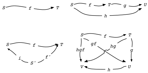
Figure 1: Top left: $f\in S\rightarrow T$. Top right: $h=g\circ f$. Bottom left: $S^{\prime}\subset S$ and $i\in S^{\prime}\rightarrow S$ is the insertion function of $S^{\prime}$ as a subset. The diagram shows $f^{\prime}=f\downarrow S^{\prime}=f\circ i$. Bottom right: $gf=g\circ f$, $hg=h\circ g$, and $hgf=h\circ(g\circ f)=(h\circ g)\circ f$.

4.5 Function composition

Definition 9 (composition)

Let $f\in S\rightarrow T$ and $g\in T\rightarrow U$. The composition $g\circ f$ of $f$ and $g$ is the function in $S\rightarrow U$ that has as map $x\mapsto g(f(x))$.

See Figure 1. We sometimes write $g\circ f$ without explicitly saying that it is defined; that is, that the target of $f$ is the source of $g$.

Example 5

For all $f\in S\rightarrow T$ we have $f\circ id_{S}=f=id_{T}\circ f$. Let $S^{\prime}$ be a subset of $S$ and let $i$ be the insertion function in $S^{\prime}\rightarrow S$. Then $f\downarrow S^{\prime}=f\circ i$. See Figure 1.

The order of $f$ and $g$ in $g\circ f$ is derived from the expression $g(f(x))$ in the definition of composition. In many situations this order seems unnatural. If the $f$ and $g$ were functional binary relations, then their composition would be written as $f;g$.

Function composition is associative: if, in addition to Definition 9, we have $h\in U\rightarrow V$, then $(h\circ g)\circ f$ and $h\circ(g\circ f)$ are the same function in $S\rightarrow V$. See Figure 1.

A useful property of composition is that if $g\circ f$ is injective, then $f$ is. For suppose that $f$ is not injective. Then there exist $x_{1}$ and $x_{2}$ in $S$ such that $x_{1}\not=x_{2}$ and $f(x_{1})=f(x_{2})$. Then we also have that $g(f(x_{1}))=g(f(x_{2}))$, so that $g\circ f$ would not be injective.

The dual counterpart of this property is that if $g\circ f$ is surjective, then $g$ is. For suppose that $g$ is not surjective. Then there is a $z$ in $U$ such that there is no $y$ in $T$ with $g(y)=z$. Then there is also no $x$ in $S$ with $g(f(x))=z$.

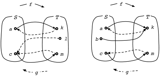
Figure 2: On the left: $g\circ f=\mbox{id}_{S}$. For this, $f$ needs to be injective, but need not be surjective. As it is not, $g$ is not uniquely determined: $g(l)$ could be $a$ and we would still have $g\circ f=\mbox{id}_{S}$. On the right: $f\circ g=\mbox{id}_{T}$. For this, $g$ needs to be injective, but need not be surjective. As it is not, $f$ is not uniquely determined: $f(b)$ could be $m$ and we would still have $f\circ g=\mbox{id}_{T}$.

Left and right inverse

Let $S$ and $T$ be nonempty sets, let $f\in S\rightarrow T$, and let $g\in T\rightarrow S$. If $\mbox{id}_{S}=g\circ f$, then we say that $f$ is a right inverse of $g$ and that $g$ is a left inverse of $f$. In this case, $f$ is injective and $g$ is surjective.

To see why, note that $\mbox{id}_{S}$ is injective and surjective. Hence, by the property of composition just introduced, $\mbox{id}_{S}=g\circ f$ implies that $f$ is injective and that $g$ is surjective.

If, in that case, $f$ is not surjective, then there exists a $y$ in $T$ such that there does not exist an $x$ in $S$ such that $f(x)=y$. For such a $y$, the value of $g$ does not affect $g\circ f$. Hence, $f$ and $\mbox{id}_{S}=g\circ f$ do not in general uniquely determine $g$.

But $\mbox{id}_{S}=g\circ f$ and $f$ surjective do determine $g$. In that case $f$ is a bijection, so that the inverse $f^{-1}$ exists. The unique $g=f^{-1}$ is a bijection as well, so that $g$ is also injective.

Conversely, injectivity of $f\in S\rightarrow T$ implies the existence of a left inverse $g\in T\rightarrow S$ such that $g\circ f=id_{S}$, which is then surjective.

4.6 Set extensions of functions

Whenever we have a function type $S\rightarrow T$, it is natural to consider the type $\mathcal{P}(S)\rightarrow\mathcal{P}(T)$. Let $f$ be in $S\rightarrow T$. We call a set extension of $f$ any function $g\in\mathcal{P}(S)\rightarrow\mathcal{P}(T)$ such that for all subsets $S^{\prime}$ of $S$ we have that $\{f(s)\mid s\in S^{\prime}\}\subset g(S^{\prime}).$

This definition suggests a partial order among the set extensions of a given $f\in S\rightarrow T$. We define $g_{0}\preceq g_{1}$ for set extensions $g_{0}$ and $g_{1}$ of $f$ iff $g_{0}(S^{\prime})\subset g_{1}(S^{\prime})$ for all subsets $S^{\prime}$ of $S$. The relation $\preceq$ is a partial order. In this partial order there is a least element. Its map is $S^{\prime}\mapsto\{f(x)\mid x\in S^{\prime}\}$ for all subsets $S^{\prime}$ of $S$. There is a greatest element in the partial order. Its map is $S^{\prime}\mapsto T$ for all subsets $S^{\prime}$ of $S$.

The least set extension of $f\in S\rightarrow T$, the one that has as map $S^{\prime}\mapsto\{f(s)\mid s\in S^{\prime}\}$, is called the canonical set extension of $f$. Conversely, the function $h$ in $\mathcal{P}(T)\rightarrow\mathcal{P}(S)$ such that for all subsets $T^{\prime}$ of $T$

$$h(T^{\prime})=\{x\in S\mid f(x)\in T^{\prime}\}$$

is the inverse set extension of $f$. Note that the inverse set extension is defined for any function, whether it is a bijection or not.

Usually, the canonical set extension of $f$ is just written as $f$, and the inverse set extension as $f^{-1}$, so that we write $f(S^{\prime})=\{f(x)\mid x\in S^{\prime}\}$ and $f^{-1}(T^{\prime})=\{x\in S\mid f(x)\in T^{\prime}\}$. Conventional notation relies on context to disambiguate $f^{-1}$, because it may mean the inverse of a bijection $f$ or it may mean the inverse set extension of an $f$ that is not necessarily a bijection.

An important property that distinguishes some set extensions is their monotonicity: $S_{1}\subset S_{2}$ implies $f(S_{1})\subset f(S_{2})$. Monotonicity gives us $f(S_{1}\cap S_{2})\subset f(S_{1})$ and $f(S_{1}\cap S_{2})\subset f(S_{2})$, so that $f(S_{1})$ and $f(S_{2})$ are both supersets of $f(S_{1}\cap S_{2})$. As $f(S_{1})\cap f(S_{2})$ is the least common superset of $f(S_{1})$ and $f(S_{2})$, we have

$$f(S_{1}\cap S_{2})\subset f(S_{1})\cap f(S_{2}).$$

But the reverse inclusion does not in general hold. For example, suppose that $f(x_{1})=f(x_{2})=y$ and $x_{1}\not=x_{2}$ and let us take $S_{1}=\{x_{1}\}$ and $S_{2}=\{x_{2}\}$. Then $y\in f(\{x_{1}\})\cap f(\{x_{2}\})$, whereas $y$ is not contained in $f(\{x_{1}\}\cap\{x_{2}\})=f(\emptyset)=\emptyset$. Injectivity of $f$ is a necessary and sufficient condition for equality.

On the other hand, we do have

$$f(S_{1})\cup f(S_{2})=f(S_{1}\cup S_{2})$$ (1)

That the left hand side is contained in the right hand side follows from monotonicity and union being the least common superset. For the reverse inclusion suppose that $y\in f(S_{1}\cup S_{2})$. Then there is an $x\in S_{1}\cup S_{2}$ such that $f(x)\in f(S_{1}\cup S_{2})$. If the $x$ is in $S_{1}$, then $f(x)$ is in $f(S_{1})$; hence in $f(S_{1})\cup f(S_{2})$. Otherwise, the $x$ is in $S_{2}$, hence $f(x)$ is in $f(S_{2})$; hence in $f(S_{1})\cup f(S_{2})$. Either way, $y\in f(S_{1})\cup f(S_{2})$. This shows that the right hand side of (1) is included in the left hand side.

For any $f$ in $S\rightarrow T$ we have

$$S^{\prime} \subset f^{-1}(f(S^{\prime}))$$

$$T^{\prime} \supset f(f^{-1}(T^{\prime}))$$

with $S^{\prime}$ and $T^{\prime}$ arbitrary subsets of $S$ and $T$. In the first case we have equality iff $f$ is injective; in the second case we have equality iff $f$ is surjective.

4.7 Enriched sets

$S$ and $T$ are the same set if and only if every element of $S$ belongs to $T$ and vice versa. Thus sets lack some properties, such as order, that are sometimes desirable in a collection. Moreover, set membership is all or nothing, not a matter of degree. Many authors consider the set-theoretic concept of a set inadequate. This leads to various proposals for enrichment of the set concept.

The method of set theory is to use functions to specify additional properties, not to enrich the concept of set itself.

“Ordered sets”

Suppose we wish to specify an order $\preceq$ among the elements of a finite set $S$. We can do this by defining a bijection $f\in n\rightarrow S$, where $n\in\mathcal{N}$. For every $x_{1}\in S$ and $x_{2}\in S$ there exist $i_{1}\in n$ and $i_{2}\in n$ such that $f(i_{1})=x_{1}$ and $f(i_{2})=x_{1}$. Then we can define $x_{1}\preceq x_{2}$ according to whether $i_{1}\leq i_{2}$.

In set theory, $S$ in combination with such an $f$ takes the place of an “ordered set”.

“Multisets”

Sometimes one considers a collection where it is not enough to say whether or not an element belongs, but one wants to say how many times it belongs. Such a collection is then called a multiset or bag.

In set theory such a requirement poses no difficulty. It is a special case of the common situation that one wants to associate an attribute with each element of a set. Suppose we have a set $S$ of objects and a set $T$ of attributes. A function $f\in S\rightarrow T$ then specifies for each $x\in S$ which of the attributes $f(x)\in T$ it has. If $T=\mathcal{N}$, then the attribute $f(x)$ can be regarded as the multiplicity of $x$.

In set theory, $S$ in combination with such an $f$ takes the place of a “multiset”.

“Fuzzy sets”

Sometimes one considers a collection where it is not enough to say whether or not an element belongs, but one wants to say how strongly it belongs.

In set theory, one would regard the required strength of belonging as an attribute. The interval $[0,1]$ of real numbers can be selected as the set of attributes. A set $S$ in combination with $f\in S\rightarrow[0,1]$ can then be regarded as a “fuzzy set”.

5 Tuples

Often a function in $S\rightarrow T$ models a process of which the input and output consist of elements of $S$ and $T$, respectively. A function $f\in S\rightarrow T$ may be used in a different way: as a method for indexing elements of $T$ using the elements of $S$ as index.

When $f$ is used in this way, then it is called a family or a tuple with $S$ as index set, of which the components are restricted to belong to $T$.

In such a situation one sometimes writes $f_{s}$ rather than $f(s)$ for the unique element of $T$ indexed by $s\in S$. Arrays in programming languages are examples of such families. Then $S=n$ and one would write $f[i]$ rather than $f(i)$ where $i\in n$.

If the index set is numerical, as in $S=n$, for some $n\in\mathcal{N}$, or $S=\mathcal{N}$, then a tuple in $S\rightarrow T$ is called a sequence. If $S=\mathcal{N}$, then the sequence is said to be infinite. If $S=n$, then we call $n$ the length of the sequence.

If we think of $T$ as an alphabet, then the functions in $n\rightarrow T$ are the strings over $T$ of length $n$. Suppose we have strings $\alpha\in m\rightarrow T$ and $\beta\in n\rightarrow T$. Then $\gamma\in(m+n)\rightarrow T$ is the concatenation of $\alpha$ and $\beta$ if the map of $\gamma$ is given by $i\mapsto\alpha(i)$ if $0\leq i<m$ and $i\mapsto\beta(i-m)$ if $m\leq i<m+n$.

5.1 Notation

Parentheses in mathematics are overloaded with meanings. There is the prime purpose of indicating tree structure in expressions. An unrelated meaning is to indicate function application, as in $f(x)$, although these two meanings seem to combine in $f(x+y)$. And then we see that a sequence $x$ in $n\rightarrow T$ is often written as $(x_{0},\ldots,x_{n-1})$. Let us at least get rid of this last variant by writing $x\in n\rightarrow T$ as $\langle x_{0},\ldots,x_{n-1}\rangle$.

Tuples need not be indexed by integers. For example, points in the Euclidean plane are reals indexed by the $X$ and $Y$ coordinates. Describing points this way corresponds to regarding a point $p$ as a tuple in $\{X,Y\}\rightarrow\mathcal{R}$. For example, a point $p$ could be such that $p_{X}=2$ and $p_{Y}=3$.

In a context where the points are thought of as being characterized by the coordinates $X$ and $Y$ one often sees $p=\langle 2,3\rangle$. Apparently, a quick switch has been made from $\{X,Y\}$ to $\{0,1\}$ as index set. We need a notation that unambiguously describes tuples with small nonnumerical index sets.

Consider tuples in $S\rightarrow T$ representing addresses. Here the index set $S$ could be

$$\{\mbox{number},\mbox{street},\mbox{city},\mbox{state},\mbox{zip}\}.$$

Such tuples can be written as lines in a table with columns labeled by the elements of the index set. The ordering of the columns is immaterial.

In this way addresses $a$, $b$, $c$, $d$, and $e$ would be described as shown in Figure 3.

	number	street	city	state	zip
$a$	19200	120th Ave	Bothell	WA	98011
$b,c$	2200	Mission College Boulevard	Santa Clara	CA	95052
	2201	C Street NW	Washington	DC	20520
$d$	36	Cooper Square	New York	NY	10003
$e$	2201	C Street NW	Washington	DC	20520

Figure 3: A sample of named and unnamed tuples.

In Figure 3, the area to the left of the double vertical line is not a column: it only serves to write the names, if any, of the tuples. The third tuple has no name; it is still a tuple. There is a tuple that has two names: $b$ and $c$. Another tuple occurs twice in the table, once with its name shown; the other time without the name.

Without a table we would have to specify laboriously $a_{\mbox{number}}=19200$, $a_{\mbox{street}}=\mbox{120th Ave},\ldots$, $b_{\mbox{number}}=2200$, $b_{\mbox{street}}=\mbox{Mission College Boulevard}$, $\ldots$, and so on. Such notation is unavoidable if tables are not available. For example in XML the tuple $a$ would be an “element” endowed with “attributes”:

<a number = "19200"     street = "120th Ave"    city = "Bothell"
   state = "WA"         zip = "98011"
>

If no tuple has a name, then one might as well omit the double vertical line, and describe the four tuples by means of the table:

number	street	city	state	zip
19200	120th Ave	Bothell	WA	98011
2200	Mission College Boulevard	Santa Clara	CA	95052
36	Cooper Square	New York	NY	10003
2201	C Street NW	Washington	DC	20520

In the same way, the point $p$ in $\{X,Y\}\rightarrow\mathcal{R}$ such that $p_{X}=2$ and $p_{Y}=3$ should be described by

	X	Y
$p$	2	3

,

instead of $p=\langle 2,3\rangle$, which would incorrectly imply $2$ as index set. We could, of course, code the $X$-coordinate as $0$ and the $Y$-coordinate as $1$, so that it would be correct to write $p$ as $\langle 2,3\rangle$. The point is that we don’t have to code familiar symbols such as $X$ and $Y$ for coordinates as something else for the sake of set-theoretic modeling.

5.2 Typed tuples

Consider a tuple with $\{\mbox{number},\mbox{street},\mbox{city},\mbox{state},\mbox{zip}\}$ as index set, representing an address. We would like to ensure that the elements indexed by number and zip belong to $\mathcal{N}$ and that the others belong to the set $\mbox{{A}}^{\ast}$ of alphabetic character strings. This is an example of typing a tuple. This involves in general associating a set with each index. That is, to type a tuple with index $I$, we use a tuple of sets with index $I$.

Example 6

Addresses could be typed by the tuple of sets

number	street	city	state	zip
$\mathcal{N}$	$\mbox{{A}}^{\ast}$	$\mbox{{A}}^{\ast}$	$\mbox{{A}}^{\ast}$	$\mathcal{N}$

Definition 10 (typing of tuples)

Let $I$ be a set of indexes, $T$ a set of disjoint sets, $\tau$ a tuple in $I\rightarrow T$, and $t$ a tuple in $I\rightarrow\cup T$. We say that $t$ is typed by $\tau$ iff we have $t(i)\in\tau(i)$ for all $i\in I$.

Because the sets in $T$ are disjoint, there is a function $\sigma\in\cup T\rightarrow T$ that maps each element $x$ of $\cup T$ to the set that is an element of $T$ to which $x$ belongs. The condition of $t$ being typed by $\tau$ can be expressed by means of function composition; see Figure 4.

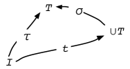
Figure 4: The tuple $t\in I\rightarrow\cup T$ is typed by $\tau\in I\rightarrow T$ iff $\tau=\sigma\circ t$.

5.3 Cartesian products

Definition 11 (Cartesian products)

Let $I$ be a set of indexes, $T$ a set of disjoint sets, and $\tau$ a tuple in $I\rightarrow T$. The Cartesian product on $\tau$, denoted $\mbox{{cart}}(\tau)$, is the set of all tuples that have $\tau$ as type.

Instead of “ $t$ is typed by $\tau$”, we can now say “ $t\in\mbox{{cart}}(\tau)$”.

Example 7

Let $\tau$ be in $\{\mbox{number},\mbox{street},\mbox{city},\mbox{state},\mbox{zip}\}\rightarrow\{\mathcal{N},\mbox{{A}}^{\ast}\},$ More specifically, let $\tau$ be equal to the tuple

number	street	city	state	zip
$\mathcal{N}$	$\mbox{{A}}^{\ast}$	$\mbox{{A}}^{\ast}$	$\mbox{{A}}^{\ast}$	$\mathcal{N}$

.

$\mbox{{cart}}(\tau)$ is the set of all tuples of type $\tau$. In this example it means that any natural number, however small or large, can occur as the element indexed by number or zip, and that any sequence of characters, in any combination, of any length, can occur as element indexed by street, city, or state. The set of actually existing addresses is a relatively small subset of $\mbox{{cart}}(\tau)$.

Example 8

Let the index set $\{X,Y\}$ contain the labels that distinguish the $X$ and $Y$ coordinates of the points in the Euclidean plane. Let $\tau$ be the tuple of sets in $\{X,Y\}\rightarrow\{\mathcal{R}\}$. Now $\mbox{{cart}}(\tau)$ is the Euclidean plane.

Often the index set of $\tau$ is $n$ for some positive natural number $n$. For this case a special notation exists for $\mbox{{cart}}(\tau)$. Let $\tau$ be in $n\rightarrow T$, where $T$ is a set of sets. The special nature of the index set allows us to write $\tau$ as $\langle\tau_{0},\ldots,\tau_{n-1}\rangle$. In the same spirit, $\mbox{{cart}}(\tau)$ may be written as $\tau_{0}\times\cdots\times\tau_{n-1}$. When $T$ consists of a single set, say, $T=\{S\}$, then $\tau\in n\rightarrow\{S\}$, and $\tau_{0}\times\cdots\times\tau_{n-1}$ may be written as $\underbrace{S\times\cdots\times S}_{n\;times}$, abbreviated as $S^{n}$.

Example 9

$S\times T=\mbox{{cart}}(\tau)$ where $\tau\in 2\rightarrow\{S,T\}$ with $\tau(0)=S$ and $\tau(1)=T$. I trust that the context prevents confusion with the binary Cartesian product $S\times T$ defined as $\{\langle x,y\rangle\mid x\in S\wedge y\in T\}$ (see Definition 2).

Example 10

A pack of playing cards can be modeled as a Cartesian product. Let $\mbox{{suit}}=\{\clubsuit,\diamondsuit,\heartsuit,\spadesuit\}$ and let $\mbox{{value}}=\{2,3,4,5,6,7,8,9,10,J,Q,K,A\}$. Let $\tau=\langle\textsc{suit},\textsc{value}\rangle$. Then the 52 elements of $\mbox{{cart}}(\tau)$, which include e.g. $\langle\heartsuit,Q\rangle$, and $\langle\spadesuit,5\rangle$, can be interpreted as playing cards. As the index set of $\tau$ is $2$, we can write $\mbox{{cart}}(\tau)$ as $\mbox{{suit}}\times\mbox{{value}}$.

Example 11

Let the index set $I=n$ for some natural number $n$ and let $T=\{\mathcal{R}\}$. Then $I\rightarrow T$ consists of one typing tuple, say $\tau$. $\mbox{{cart}}(\tau)$ consists of the points in Euclidean $n$-space and we write $\mathcal{R}^{n}$ instead of $\mbox{{cart}}(\tau)$.

5.4 Functions and Cartesian products

We have considered functions $f$ in $S\rightarrow T$. These have one argument $x$ in $S$ that gets mapped into $f(x)\in T$. $S$ or $T$, or both, may be a Cartesian product.

Suppose $S=\mbox{{cart}}(\tau)$, with $\tau\in I\rightarrow U$. The argument of $f$ is a tuple that is not necessarily indexed by numbers. However, if $I=n$, then we have $f\in U_{0}\times\cdots\times U_{n-1}\rightarrow T$ and $f$-values look like $f(\langle u_{0},\ldots,u_{n-1}\rangle)$, usually written as $f(u_{0},\ldots,u_{n-1})$, where $u_{0}\in U_{0},\ldots,u_{n-1}\in U_{n-1}$. This is an alternative to Currying for modeling multi-argument functions.

It can also happen that the target set $T$ of a function $f$ in $S\rightarrow T$ is a Cartesian product. In such a case it may be more natural to think of $f$ as a tuple $f^{\prime}$ of functions. Suppose that $f$ is in $S\rightarrow\mbox{{cart}}(\tau)$ with $\tau\in I\rightarrow U$, where $U$ is a set of sets. Thus, for each $x\in S$, we have that $f(x)$ is a tuple with index set $I$. For each $i\in I$, $(f(x))_{i}$ is an element of this tuple.

One can also think of such an $f$ as a tuple $f^{\prime}$ of functions with index set $I$. For each $i\in I$, we define the element $f^{\prime}_{i}$ of the tuple $f^{\prime}$ as the function in $S\rightarrow\tau_{i}$ with map $x\mapsto(f(x))_{i}$.

For every function $f$ that has a Cartesian product as target, there is a tuple $f^{\prime}$ of functions uniquely determined as shown above. Conversely, for every tuple of functions that have the same source, the above shows the uniquely determined function with this source that has tuples as values.

5.5 Projections

Consider a sequence $s=\langle a,b,c,d,e\rangle$ in $5\rightarrow\mbox{{A}}$, where A is a set of alphabetical characters. Which, if any, of the following is a “subsequence” of $s$: $\langle b,c,d\rangle$, $\langle a,c,e\rangle$, $\langle e,c,a\rangle$, or $\langle a,a,c\rangle$? Authors’ opinions differ.

We saw that the definition of function leads in a natural way to the notion of restriction. Sequences, being tuples, being functions, therefore also have restrictions. In set theory, subtuples are modeled as restrictions:

Definition 12 (subtuple)

If $S^{\prime}\subset S$, then $f\downarrow S^{\prime}$ is the subtuple on $S^{\prime}$ of the tuple $f$ in $S\rightarrow T$.

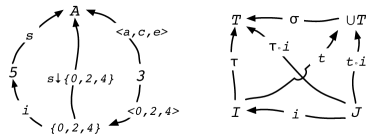
Figure 5: Left: See Example 12. Right: See Definition 14. The fact that $t$ is typed by $\tau$ is expressed by the fact that $\tau=\sigma\circ t$. It follows that $\tau\circ i=\sigma\circ t\circ i$.

Example 12

Let $s=\langle a,b,c,d,e\rangle$. We could restrict the index set of $s$, which is $5$, to $S^{\prime}=\{0,2,4\}$ and get as a subtuple of $s$ the restriction $s\downarrow S^{\prime}$, which is 0 2 4 a c e , and which is not $\langle a,c,e\rangle$. In fact, we have that $\langle a,c,e\rangle=(s\downarrow S^{\prime})\circ\langle 0,2,4\rangle$, if the target of $\langle 0,2,4\rangle$ is $\{0,2,4\}$. See Figure 5.

Though tuples are functions, we saw that they come with their own terminology. We saw that it is “index set” instead of “source” and “subtuple” instead of restriction. In fact, there is additional specialized terminology for tuples.

Definition 13 (projection)

Let $t$ be a tuple with index set $I$ and let $J$ be a subset of $I$. The projection $\pi_{J}(t)$ of $t$ on $J$ is the subtuple $t\downarrow J$ of $t$.

Thus we have $\pi_{\{0,2,4\}}(\langle a,b,c,d,e\rangle)=\begin{tabular}[]{l|l|l}0&2&4\\ \hline\cr a&c&e\end{tabular}$.

When the projection is on a singleton set of indexes, the result is a singleton tuple. Rather than writing $\pi_{\{3\}}(\langle a,b,c,d,e\rangle)=\begin{tabular}[]{l}3\\ \hline\cr d\end{tabular}$, we may write the singleton set of indexes as the index by itself: $\pi_{3}(\langle a,b,c,d,e\rangle)=\begin{tabular}[]{l}3\\ \hline\cr d\end{tabular}$.

If a tuple $t$ has type $\tau$, then the subtuples of $t$ are typed in an obvious way. This observation suggests the definition below.

Definition 14 (subtype)

Let $T$ be a set of disjoint sets, $I$ an index set, $J$ a subset of $I$, and $\tau$ a type in $I\rightarrow T$. We define $\tau\downarrow J$ to be the subtype of $\tau$ determined by $J$.

Let now $t\in I\rightarrow\cup T$ be a tuple typed by $\tau$. It is easy to see that the subtuple $t\downarrow J$ of $t$ is typed by the subtype $\tau\downarrow J$ of $\tau$. Observe that, if $i\in J\rightarrow I$ is the insertion function, then $t\downarrow J=t\circ i$. In Figure 5 we see that $\tau\downarrow J=\sigma\circ(t\downarrow J)$. This shows that if we want to say that $t\downarrow J$ is typed by $\tau\downarrow J$, then we can say it with arrows.

A projection that is defined for an individual tuple is also defined, as canonical set extension, on a set of tuples that have the same type. Consider for example a Cartesian product. It is a set of tuples of the same type. Therefore $\pi_{J}(\mbox{{cart}}(\tau))$ is defined by canonical set extension to be equal to $\{\pi_{J}(t)\mid t\in\mbox{{cart}}(\tau)\}$. These are all the tuples of type $\pi_{J}(\tau)$, so by definition equal to $\mbox{{cart}}(\pi_{J}(\tau))$. Thus we see that a projection of a Cartesian product is itself a Cartesian product.

6 Relations

In Section 3 we defined binary relations. In this section we define a kind of relation that can hold between any number of arguments. We call these “relation”. Whenever we refer to a binary relation, we should always qualify it as such. The generality of relations implies that some of them hold between two arguments. But these are still relations and not binary relations. The situation is similar to the trees in Knuth’s Art of Programming [7]. He defines binary trees and trees in such a way that binary trees are not a special case of trees.

Relations are specified by means of sets consisting of the tuples containing the objects that are in the relation. It is not enough for the sizes of these tuples to be the same. Just as the source and the target are parts of the specification of a function, a relation is most useful as a concept when its tuples have the same type. Therefore this type is part of the specification of a relation.

Definition 15 (relation)

A relation is a pair $\langle\tau,E\rangle$ where $\tau$, the signature, or the type, of the relation, is a tuple of type $I\rightarrow T$, where $T$ is a set of sets, and $E$, the extent of the relation, is a subset of $\mbox{{cart}}(\tau)$.

Example 13

$\langle\tau,E\rangle$ where $\tau$ has the empty set as index set. $\mbox{{cart}}(\tau)$ has one element, the empty tuple. There are two possibilities for $E$: the empty set and the singleton set containing the empty tuple.

The following example emphasizes the distinction between a relation and a binary relation.

Example 14

A relation $\langle\tau,E\rangle$ with $\tau\in 2\rightarrow T$ can be represented without loss of information by the binary relation $\langle\tau(0),\tau(1),\{\langle t_{0},t_{1}\rangle\mid t\in E\}\rangle$. Conversely, let $\langle S,T,E\rangle$ be a binary relation and let $\tau\in 2\rightarrow\{S,T\}$ be such that $\tau_{0}=S$ and $\tau_{1}=T$. This binary relation is represented without loss of information as the relation $\langle\tau,F\rangle$ where $F=\{t\in\mbox{{cart}}(\tau)\mid\langle t_{0},t_{1}\rangle\in E\}.$

The following example shows that set theory is of potential interest to databases.

Example 15

Let $\tau$ be as in Example 7. The actually existing addresses are but a relatively small subset $E$ of $\mbox{{cart}}(\tau)$. The relation $\langle\tau,E\rangle$ is a relational format for the information represented by this set of addresses.

Example 16

The Euclidean plane is a set of tuples that have index set $\{X,Y\}$ and where both elements are reals. That is, the Euclidean plane is $\mbox{{cart}}(\tau)$, where $\tau$.

A figure in the Euclidean plane is a subset of the Euclidean plane. So every figure in the Euclidean plane is a relation of type $\{X,Y\}\rightarrow\{\mathcal{R}\}$. For example, the relation

$$\langle\tau,\{p\in\mbox{{cart}}(\tau)\mid p_{X}^{2}+p_{Y}^{2}=1\}\rangle$$

is the unit circle with the origin as centre.

6.1 Set-like operations

Among relations of the same type certain relational operations are defined that mirror set operations:

$$\langle\tau,E_{1}\rangle\cup\langle\tau,E_{2}\rangle \stackrel{{\scriptstyle def}}{{=}} \langle\tau,E_{1}\cup E_{2}\rangle$$

$$\langle\tau,E_{1}\rangle\cap\langle\tau,E_{2}\rangle \stackrel{{\scriptstyle def}}{{=}} \langle\tau,E_{1}\cap E_{2}\rangle$$

$$\langle\tau,E_{1}\rangle\setminus\langle\tau,E_{2}\rangle \stackrel{{\scriptstyle def}}{{=}} \langle\tau,E_{1}\setminus E_{2}\rangle$$

6.2 Relations with named tuples

The extent of a relation $\langle\tau,E\rangle$ is the set of tuples $E$. These tuples are not named or ordered. Naming of the tuples can be achieved by a set $S$ of names and a function $f$ in $S\rightarrow E$. If we want to name all tuples, $f$ needs to be surjective.

It is also be possible to name the tuples of a relation by means of a subset $I^{\prime}$ of $I$ (where $I$ is the index set of $\tau$), if $t\downarrow I^{\prime}$ uniquely identifies $t$. That is, if $t_{0}\downarrow I^{\prime}=t_{1}\downarrow I^{\prime}$ implies, for all $t_{0},t_{1}\in E$, that $t_{0}=t_{1}$. Sometimes such an $I^{\prime}$ is a singleton set $\{i\}$. A common example is where $E$ consists of tuples $t$ describing employees and $t_{i}$ is the social insurance number.

6.3 Projections and cylinders

Recall that projections are defined (Definition 13) as restrictions of tuples. Canonical set extensions of projections are therefore defined on sets of tuples. As extents of relations are sets of tuples, projections are also defined, as canonical set extensions, on extents of relations.

Definition 16 (projection)

Let $\tau$ be in $I\rightarrow T$, where $T$ is a set of disjoint sets and $I$ is an index set. The projection on $J$ of the relation $\langle\tau,E\rangle$ is written $\pi_{J}(\langle\tau,E\rangle)$ and is defined to be the relation $\langle\tau\downarrow J,\{t\downarrow J\mid t\in E\}\rangle$.

Example 17

If we have a relation $r=\langle\tau,E\rangle$ where $\tau$ is

number	street	city	state	zip
$\mathcal{N}$	$\mbox{{A}}^{\ast}$	$\mbox{{A}}^{\ast}$	$\mbox{{A}}^{\ast}$	$\mathcal{N}$

and $E$ is the set of tuples that represent addresses of subscribers, then $\pi_{\{\mbox{city},\mbox{state}\}}(r)$ is a relational format for the cities where there is at least one subscriber.

Example 18

Let $r$ be the relation $\langle\tau,E\rangle$ where $\tau=3\rightarrow\{\{a,b\}\}$ and $E=\{\langle a,a,a\rangle,\langle a,a,b\rangle,\langle b,a,b\rangle\}$.

An example of a projection is

$$\pi_{2}(r)=\langle 2\rightarrow\{\{a,b\}\},\{\langle a,a\rangle,\langle b,a\rangle\}\rangle$$

We cannot represent the extent of, e.g., $\pi_{\{0,2\}}(r)$ with angle brackets because the angle brackets presuppose an index set in the form of $n$. Instead we say,

$$\pi_{\{0,2\}}(r)=\langle\{0,2\}\rightarrow\{\{a,b\}\},E\rangle$$

where $E=\begin{array}[]{l|l}0&2\\ \hline\cr a&a\\ a&b\\ b&b\end{array}$.

Projections are more often used as canonical set extensions on sets of tuples than on individual tuples. As projections are typically not injective, they typically do not have an inverse. But every function does have an inverse set extension. The inverse set extensions of projections are especially useful.

Let $I$ be an index set with a subset $J$. If $S$ is a set of tuples with index set $J$, then we can ask: What tuples $t$ with index set $I$ are such that $\pi_{J}(t)\in S$? This is the definition of inverse set extension: it is defined for all functions, projections or not. So

$$\pi^{-1}_{J}(S)=\{t\mid\pi_{J}(t)\in S\}.$$

Example 19

In Example 18, $\pi^{-1}_{\{0,1\}}$ applied to the extent of $\pi_{\{0,1\}}(r)$ and $\pi^{-1}_{\{0,2\}}$ applied to the extent of $\pi_{\{0,2\}}(r)$ are, respectively,

$$\{\langle a,a,a\rangle,\langle a,a,b\rangle,\langle b,a,a\rangle,\langle b,a,b\rangle\}$$

$$\{\langle a,a,a\rangle,\langle a,b,a\rangle,\langle a,a,b\rangle,\langle a,b,b\rangle,\langle b,a,b\rangle,\langle b,b,b\rangle\}$$

Given a relation $r$, one can also wonder about relations that have $r$ as projection. There is a largest such, which is the “cylinder” on $r$. This gives the idea; to get the signatures right, see the following definition.

Definition 17 (cylinder)

For $i\in\{0,1\}$, let $\tau_{i}$ be in $I_{i}\rightarrow T_{i}$, such that $\tau_{0}$ and $\tau_{1}$ are summable; $T_{i}$ is a set of sets. Let $\langle\tau_{0},E_{0}\rangle$ be a relation. The cylinder in $I_{0}\cup I_{1}$ on $\langle\tau_{0},E_{0}\rangle$ is written as $\pi^{-1}_{I_{0}\cup I_{1}}(\langle\tau_{0},E_{0}\rangle)$ and is defined to be relation

$$\langle\tau_{0}+\tau_{1},\{t\in\mbox{{cart}}(\tau_{0}+\tau_{1})\mid t\downarrow I_{0}\in E_{0}\}\rangle.$$

The notation $\pi^{-1}$ suggests some kind of inverse of projection. The suggestion is inspired by facts such as $\pi_{I_{0}}(\pi^{-1}_{I_{0}\cup I_{1}}(\langle\tau_{0},E_{0}\rangle))=\langle\tau_{0},E_{0}\rangle$.

Example 20

Consider $\mbox{{cart}}(\tau)$, with $\tau$ in $\{X,Y,Z\}\rightarrow\{\mathcal{R}\}$, and think of it as the three-dimensional Euclidean space. Let the relation $r$ be $\langle\tau,\{t\in\mbox{{cart}}(\tau)\mid t_{X}^{2}+t_{Y}^{2}+t_{Z}^{2}\leq 1\}\rangle$, which is the unit sphere with centre in the origin. The projections

$$\pi_{\{X,Y\}}(r) = \langle\tau\downarrow\{X,Y\},\{t\in\pi_{\{X,Y\}}\mbox{{cart}}(\tau)\mid t_{X}^{2}+t_{Y}^{2}\leq 1\}\rangle$$

$$\pi_{\{Z,Y\}}(r) = \langle\tau\downarrow\{Z,Y\},\{t\in\pi_{\{Z,Y\}}\mbox{{cart}}(\tau)\mid t_{Z}^{2}+t_{Y}^{2}\leq 1\}\rangle$$

$$\pi_{\{Z,X\}}(r) = \langle\tau\downarrow\{Z,X\},\{t\in\pi_{\{Z,X\}}\mbox{{cart}}(\tau)\mid t_{Z}^{2}+t_{X}^{2}\leq 1\}\rangle$$

can be thought of as the two-dimensional projections of the sphere.

The one-dimensional projections

$$\pi_{X}(r) = \langle\tau\downarrow\{X\},\{t\in\pi_{X}\mbox{{cart}}(\tau)\mid t_{X}^{2}\leq 1\}\rangle$$

$$\pi_{Y}(r) = \langle\tau\downarrow\{Y\},\{t\in\pi_{Y}\mbox{{cart}}(\tau)\mid t_{Y}^{2}\leq 1\}\rangle$$

$$\pi_{Z}(r) = \langle\tau\downarrow\{Z\},\{t\in\pi_{Z}\mbox{{cart}}(\tau)\mid t_{Z}^{2}\leq 1\}\rangle$$

can be thought of as the one-dimensional projections of the sphere.

The cylinder $\pi_{X}^{-1}(\pi_{X}(r))$ looks like an infinite slab bounded by two planes parallel to the $Y,Z$-plane through the points with $Y$ and $Z$ coordinates 0 and with $X$ coordinates $-1$ and $+1$. This slab is just wide enough to contain the sphere.

$$\pi_{X}^{-1}(\pi_{X}(r))\cap\pi_{Y}^{-1}(\pi_{Y}(r))\cap\pi_{Z}^{-1}(\pi_{Z}(r))$$

is the intersection of three such slabs perpendicular to each other, so it is the smallest cube with edges parallel to the coordinate axes that contains the sphere. It is a Cartesian product.

The cylinder $\pi_{\{X,Y\}}^{-1}(\pi_{\{X,Y\}}(r))$ looks like, well, a cylinder. Its axis is parallel to the $Z$ axis. The unit disk in the $X,Y$-plane with its centre at the origin is a cross-section.

$$\pi_{\{X,Y\}}^{-1}(\pi_{\{X,Y\}}(r))\cap\pi_{\{Z,X\}}^{-1}(\pi_{\{Z,X\}}(r))\cap\pi_{\{Z,Y\}}^{-1}(\pi_{\{Z,Y\}}(r))$$

is the intersection of three such cylinders. It is a body bounded by curved planes that properly contains the sphere $r$ and is properly contained in the box.

Definition 18 (join)

For $i\in\{0,1\}$ let there be relations $\langle\tau_{i},E_{i}\rangle$, with $\tau_{i}\in I_{i}\rightarrow T_{i}$ and $T_{i}$ a set of disjoint sets. If $\tau_{0}$ and $\tau_{1}$ are summable, then the join of $\langle\tau_{0},E_{0}\rangle$ and $\langle\tau_{1},E_{1}\rangle$ is written as $\langle\tau_{0},E_{0}\rangle\Join\langle\tau_{1},E_{1}\rangle$ and defined to be $\pi^{-1}_{I_{0}\cup I_{1}}(\langle\tau_{0},E_{0}\rangle)\cap\pi^{-1}_{I_{0}\cup I_{1}}(\langle\tau_{1},E_{1}\rangle)$.

The intersection in this definition is defined because of the assumed summability of $\tau_{0}$ and $\tau_{1}$. The signature of $\langle\tau_{0},E_{0}\rangle\Join\langle\tau_{1},E_{1}\rangle$ is $\tau_{0}+\tau_{1}$.

7 Application to relational databases

Codd [3] proposed to represent the information in “large banks of formatted data” as a collection of relations. This proposal has been so successful that databases are ubiquitous and that most of these conform to Codd’s relational model for data. The success of the relational model is due to the fact that its mathematical nature has made more manageable the complexity that would have prevented the earlier models to support the enormous growth that databases have experienced.

I have selected relational databases as example of an application in computer science where elementary set theory is useful. This is because the notion of relation is far from clear in the early database literature. As examples I have selected Codd’s original paper [3] and Ullman’s widely quoted textbook [11].

7.1 The relational model according to Codd

In Codd [3] we find the following definition, the original one, in section 1.3 “A Relational View of Data”:

The term relation is used here in its accepted mathematical sense. Given sets $S_{1},\ldots,S_{n}$ (not necessarily distinct), $R$ is a relation on these $n$ sets if it is a set of $n$-tuples each of which has its first element from $S_{1}$, its second element from $S_{2}$, and so on. We shall refer to $S_{j}$ as the $j$th domain of $R$.

Note that $S_{j}$, not $j$, is the domain. Thus $S_{i}$ and $S_{j}$ may be the same set, even though $i\not=j$. The above quote continues with:

For expository reasons, we shall frequently make use of an array representation of relations, but it must be remembered that this particular representation is not an essential part of the relational view being expounded. An array which represents an $n$-ary relation $R$ has the following properties:

1. Each row represents an $n$-tuple of $R$.

2. The ordering of rows is immaterial.

3. All rows are distinct.

4. The ordering of columns is significant — it corresponds to the ordering $S_{1},\ldots,S_{n}$ of the domains on which $R$ is defined (see, however, remarks below on domain-ordered and domain-unordered relations).

5. The significance of each column is partially conveyed by labeling it with the name of the corresponding domain.

Codd gives as example of such an array the one shown in Figure 6. He observes that this example does not illustrate why the order of the columns matters. For that he introduces the one in Figure 7.

  supply (supplier part project quantity) 1 2 5 17 $\ldots$ $\ldots$ $\ldots$ $\ldots$  

Figure 6: Codd’s first example: domains all different.

  component (part part quantity) 1 5 9 $\ldots$ $\ldots$ $\ldots$  

Figure 7: Codd’s second example: domains not all different.

He explains Figure 7 as follows.

$\ldots$ two columns may have identical headings (indicating identical domains) but possess distinct meanings with respect to the relation.

We can take it that in Figure 7 we have $n=3$, $S_{1}=S_{2}=\mbox{ part}$, and $S_{3}=\mbox{ quantity}$. As $S_{1},\ldots,S_{n}$ need not all be different, columns can only identified by $\{1,\ldots,n\}$.

Codd goes on to point out that in practice $n$ can be as large as thirty and that users of such a relation find it difficult to refer to each column by the correct choice among the integers $1,\ldots,30$. According to Codd, the solution is as follows.

Accordingly, we propose that users deal, not with relations, which are domain-ordered, but with relationships, which are domain-unordered.

One problem is the term “domain-ordered”. The term suggests that the relation is ordered by the domains $S_{1},\ldots,S_{n}$. But, as Codd warns us, these sets are necessarily distinct. If there are fewer than $n$ domains, then they cannot order the relation.

Another problem with this passage is the introduction of “relationships” as distinct from “relations”. Codd notes in his description of the relational view of data that “the term relation is used in its accepted mathematical sense”. He would have had a hard time to find an accepted mathematical sense for the distinction between “relation” and “relationship”.

Codd started out with the bold idea that the data that need to be managed in practice can be organized as relations “in their accepted mathematical sense”. Within one page he was forced to retract from this promising start to get bogged down in the murky area of “domain-ordered relations” versus “domain-unordered relationships”.

The cause of the difficulty is that Codd seemed to regard it as somehow unmathematical for the index set $I$ to be anything that differs from $\{1,\ldots,n\}$. In this paper, the exposition leading up to Definition 15 is intended to ensure that one is not even tempted to entertain such a misconception.

7.2 The relational model according to Ullman

The reader may have thought that the difficulties in Codd [3] would soon be straightened out as this original proposal became mainstream computer science, and, as such, the subject of widely quoted textbooks. Let us look at one of these, the one by J.D. Ullman [11].

[11] introduces “The Set-Theoretic Notion of a Relation” (page 43), a notion there also called “the set-of-lists” notion of a relation. This is distinguished from “An Alternative Formulation of Relations”, one that is called “relation in the set-of-mappings sense”.

The set-list-lists notion of a relation is any subset of the Cartesian product $D_{1}\times\cdots\times D_{k}$, where $D_{1},\ldots,D_{k}$ are domains. While Codd was careful to say that the domains need not be distinct, [11] says that there are $k$ domains. But this is probably not intended. [11] uses attributes $A_{1},\ldots,A_{k}$ to name the columns of a tabular representation of a relation. [11] does not say whether these are distinct, but that is probably intended.

In the set-of-lists type of relation, columns are named by the indexes $1,\ldots,k$. Apparently, the attributes $A_{1},\ldots,A_{k}$ are redundant comments on the columns.

Starting on page 44, in the “Alternative Formulation” section, [11] makes the observation that the attributes can be used to index the domains instead of the indexes $\{1,\ldots,k\}$ in the set-of-lists type of relation. When the indexes are attributes, one has a “relation in the set-of-mappings sense”. This kind of relation is illustrated with examples rather than defined.

[11] observes that in the practice of database use, relations are sets of mappings. This make one wonder why the other kind, with its redundant numerical indexes, was introduced. The answer comes on page 53, in the section on relational algebra.

Recall that a relation is a set of $k$-tuples for some $k$, called the arity of the relation. In general, we give names (attributes) to the components of tuples, although some of the operations mentioned below, such as union, difference, product, and intersection, do not depend on the names of the components. These operations do depend on there being a fixed, agreed-upon order for the attributes; i.e. they are operations on the list style of tuples rather than the mapping (from the attribute names to values) style.

As we saw earlier, these operations do not depend on the index set of the type $\tau$ of a relation $\langle\tau,E\rangle$ having “a fixed, agreed-upon order” for its elements.

Definition 15 obviates the need for Codd’s distinction between “domain-ordered” and “domain-unordered” relations and for Ullman’s distinction between “sets-of-lists type relations” and “relations in the sets-of-mappings sense”. Codd’s idea of a relational format for data was a promising one, but the special case of relations as subsets of $D_{1}\times\cdots\times D_{n}$ is too special. It is perhaps not too late to revisit Codd’s idea with relations according to Definition 15.

7.3 A reconstruction of the relational model according to set theory and logic

Let us now see what the relational model for data would look like to someone who knows some set theory and who was only told the general idea of [3] without the details as worked out by Codd. We first look how data are stored, then how they are queried. Finally, in this section, we introduce a relational operation that facilitates querying.

7.3.1 Relations are repository for data

We have to start with what is implicit in the very idea of a database, relational or not. The information to be stored in a database concerns various aspects of things like employees in an organization, parts of an airplane, books in library, and so on. The general pattern seems to be that a database describes a collection of objects.

There is no limit to the information one can collect about an object as it exists in reality. Hence one performs an act of abstraction by deciding on a set of attributes that apply to the object and one determines what is the value of each attribute for this particular object. A consequence of this abstraction is that it cannot distinguish between objects for which the attributes have the same value. The set of attributes has to be comprehensive enough that this does not matter for the purpose of the database. That is, within the microcosm of the database, one assumes that Leibniz’s principle of Identity of Indiscernibles holds.

The foregoing is summarized in the first of the following points. The remaining points constitute a reconstruction of the main ideas of a relational database as suggested by the first point.

1. A database is a description of a world populated by objects. For each object, the database lists the values of the applicable attributes.

2. The database presupposes a set of attributes, and for each attribute, a set of allowable values for this attribute. Such sets of admissible values are called domains. Let $A$ be the set of attributes and let $T$ be a set of disjoint domains. As each attribute has a uniquely determined domain, this information is expressed by a function, say $\tau$, that is of type $A\rightarrow T$.

3. Not all attributes apply to every object. Hence, two objects may be similar in the sense that the same set of attributes applies to both. Let us say that objects that are similar in this sense belong to the same class. Hence a class is characterized by the subset of $A$ that contains the attributes of the objects in the class.

4. The description of each object is an association of a value with each attribute that is applicable to the object. That is, the object is represented by a tuple that is typed by $\tau\downarrow I$, where $I$ is the set of attributes of the class to which the object belongs.

5. The objects of a class are described by tuples of the same type. As tuples of the same type are a relation, the class is a relation of that type. As objects need not belong to the same class, a database consists in general of multiple relations $\langle\tau\downarrow I_{0},E_{0}\rangle,\ldots,\langle\tau\downarrow I_{n-1},E_{n-1}\rangle$, where $I_{0},\ldots,I_{n-1}$ are the attribute sets of the classes.

6. The life cycle of a database includes a design phase followed by a usage phase. In the design phase $A$, $T$, and $\tau\in A\rightarrow T$ is determined, as well as the subsets $I_{0},\ldots,I_{n-1}$ of $A$. This is the database scheme. In the usage phase the extents $E_{0},\ldots,E_{n-1}$ are added and modified. With the extents added, we have a database instance.

Note that the set of attributes of one class might be included in another. This suggests a hierarchy of classes. Note also that nothing is said about the nature of the values that the attributes might take. Values might be restricted to simple values like numbers or strings. Or they could be tuples of one of the relations.

It would seem that whether to include these possibilities in a relational database would be a matter of trading off flexibility in modeling against simplicity and efficiency in implementation. Not so: these possibilities amount to an object-relational database, the desirability of which is subject to heated controversy.

7.3.2 Queries, relational algebras, query languages

According the relational model, relations are not only used as format for the data stored in a database, but also as format for queries; that is, for selections of data to be retrieved from the database. Thus the results of queries are relations. These relations depend on those that are stored in the database and must therefore be the result of operations on them. Let us see how we can use the operations introduced so far.

$\mbox{ {suppliers}}=$

sid	sname	city
321	lee	tulsa
322	poe	taos
323	ray	tulsa

    $\mbox{ {parts}}=$ pid pname sid pqty 213 hose 322 13 214 tube 321 6 215 shim 322 18

$\mbox{ {projects}}=$

rid	pid	rqty
132	215	2
133	214	11
134	213	18

Figure 8: The relations for Example 21.

SELECT PNAME, CITY
FROM SUPPLIERS, PARTS, PROJECTS
WHERE PARTS.PID = PROJECTS.PID AND SUPPLIERS.SID = PARTS.SID
      AND RQTY <= PQTY

Figure 9: An SQL query to the relations in Figure 8.

Example 21 (Shim in Taos)

Consider the relations shown in the tables in Figure 8. Each table consists of a line of headings followed by the line entries of the tables. The line entries represent the tuples of the relations. Each table has three such lines.

The following abbreviations are used. In the suppliers table, sid for supplier ID, sname for supplier name, and city for supplier city. In the parts table, pid for part ID, pname for part name, and pqty for part quantity on hand. In the projects table, rid for project ID and rqty for part quantity required.

We want to know the part names and cities in which there is a supplier with a sufficient quantity on hand for at least one of the projects.

The relation specified by the SQL query in Figure 9 can be specified with relations according to Definitions 15, and with projection and join according to Definitions 16 and 18, respectively.

Let the tables in Figure 8 be the relations $\mbox{ {suppliers}}=\langle\tau_{0},E_{0}\rangle$, $\mbox{ {parts}}=\langle\tau_{1},E_{1}\rangle$, and $\mbox{ {projects}}=\langle\tau_{2},E_{2}\rangle$. In addition, there is a relation in the query for which there is no table, namely the less-than-or-equal relation. Mathematically, there is no reason to treat it differently from the relations stored in tables. Hence, we also include it as $\mbox{ {leq}}=\langle\tau_{3},E_{3}\rangle$.

The index sets of $\tau_{0}$, $\tau_{1}$, $\tau_{2}$ are the sets of the column headings of the tables for suppliers, parts, and projects, respectively: for $\tau_{0}$ the index set is $\{\mbox{ {sid}},\mbox{ {sname}},\mbox{ {city}}\}$, for $\tau_{1}$ it is $\{\mbox{ {pid}},\mbox{ {pname}},\mbox{ {sid}},\mbox{ {pqty}}\}$, for $\tau_{2}$ it is $\{\mbox{ {rid}},\mbox{ {pid}},\mbox{ {rqty}}\}$. For $\tau_{3}$ it is $\{\mbox{ {rqty}},\mbox{ {pqty}}\}$.

The extents $E_{0}$, $E_{1}$, and $E_{2}$ are as described in Figure 8. Moreover, $E_{3}=\{t\in\mbox{{cart}}(\tau_{3})\mid t_{\mbox{ {rqty}}}\leq t_{\mbox{ {pqty}}}\}$.

Consider now the relation

$$\pi_{\{\mbox{ {pname}},\mbox{ {city}}\}}=\mbox{ {suppliers}}\Join\mbox{ {parts}}\Join\mbox{ {projects}}\Join\mbox{ {leq}}.$$ (2)

For the relations to be joinable, the signatures $\tau_{0}$, $\tau_{1}$, $\tau_{2}$, and $\tau_{3}$ have to be summable. That is, for any elements common to their source sets, they have to have the same value. For example, the source sets of $\tau_{0}$ and $\tau_{1}$ have sid in common. They both map sid to its domain, which is the set of supplier IDs. Therefore $\tau_{0}$ and $\tau_{1}$ are summable; hence $\mbox{ {cities}}\Join\mbox{ {parts}}$ is defined (Definition 18). Similarly with the other joins in the expression (2), which has as value the relation described by the SQL query in Figure 8.

In the query in Example 21 every relation occurs at most once. In the following example we consider a query where this is not the case.

Example 22 (Mary, Alan)

In Figure 10 we show a table specifying a relation consisting of tuples of two elements where one is a parent of the other. It is required to identify pairs of persons who are in the grandparent relation.

$\textsc{pc}=$ parent child mary john john alan mary joan

Figure 10: Relation for Example 22.

What distinguishes this query from the one in Example 21 is that the relations do not occur in the join as given, but are derived from the given relation. On the basis of the derived relations we create one in which the pairs are in the grandparent relation. In one of the SQL dialects this would be:

SELECT PC0.PARENT, PC1.CHILD
FROM   PC AS PC0, PC AS PC1
WHERE  PC0.CHILD = PC1.PARENT

In this query, the derived tables are obtained via the linguistic device of renaming pc to $\textsc{pc}_{0}$ and $\textsc{pc}_{1}$.

7.3.3 An additional relational operation

Do we have to introduce a special-purpose language to handle a simple query such as this one? In the following we show how an additional relational operation, “filtering”, is sufficient to handle, in combination with projection and join, not only this query, but more generally, to write relations expressions that mimic the queries of a powerful query language such as Datalog [8].

The filtering operation acts on a relation and a tuple and results in a relation. Let the relation be $\langle\tau,E\rangle$ with $\tau\in I\rightarrow T$ and $T$ a set of disjoint sets. Let the tuple be $p\in I\rightarrow V$, where $V$ is a set of objects that we think of as placeholders. In similar situations such placeholders are often called “variables”, which is fine, as long as we remember that they are elements of a set, and that there is nothing linguistic about them.

For each such tuple $p$ we can ask: is there a $t\in E$ such that $t=s\circ p$ for some $s\in V\rightarrow\cup T$? In that case we include $s$ in the extent $E^{\prime}$ of a relation $\langle\varphi,E^{\prime}\rangle$. See Figure 11.

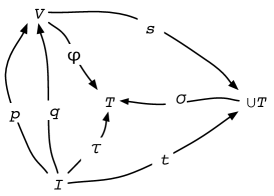
Figure 11: Sets and functions involved in filtering.

Definition 19 (filtering)

Let $\tau$ be in $I\rightarrow T$, where $T$ is a set of disjoint sets and $I$ is an index set. Let $p\in I\rightarrow V$ be a tuple. Let $\varphi\in V\rightarrow T$ be such that $\tau=\varphi\circ p$. The filtering by $p$ of the relation $\langle\tau,E\rangle$ is written $\langle\tau,E\rangle:p$ and is defined to be the relation $\langle\varphi,\{s\in p(I)\rightarrow\cup T\mid\exists t\in E.\;t=s\circ p\}\rangle$.

The condition $\tau=\varphi\circ p$ ensures that the variables in $V$ are typed compatibly with $\tau$.

Example 23

Let $I=3$, $T=\{\mathcal{R}\}$, $V=\{x,y,z\}$, $\tau\in I\rightarrow T$, and $E=\{\langle u,v,w\rangle\in\mathcal{R}^{3}\mid u\times v=w\}$. Let $p=\langle x,x,z\rangle$. What is $\langle\tau,E\rangle:p$?

In this example we use the filtering operation to obtain the squaring relation as a special case of the multiplication relation. As $T$ is a singleton set, there is only one possibility for $\tau$, and this is $\langle\mathcal{R},\mathcal{R},\mathcal{R}\rangle$. The same holds for $\varphi$. In this way, $\langle\tau,E\rangle$ is the multiplication relation over the reals.

Definition 19 now implies that the extent of $\langle\tau,E\rangle:p$, the result of applying filtering with $p$ to $\langle\tau,E\rangle$, is $\{s\in\{x,z\}\rightarrow\mathcal{R}\mid s_{x}^{2}=s_{z}\}$. This can be explained as follows. We need to find all $s\in\{x,z\}\rightarrow\mathcal{R}$ such that there exists a $t\in E$ with $t=s\circ p$. Now, $t=s\circ p$ implies that $t_{0}=(s\circ p)_{0}=s_{p_{0}}=s_{x}$. Similarly, $t_{1}=(s\circ p)_{1}=s_{p_{1}}=s_{x}$.

That is, $t=s\circ p$ has a solution $s$ iff $t_{0}=t_{1}$. Indeed, $p=\langle x,x,z\rangle$ can be regarded as a pattern that a $t\in E$ may or may not conform to. By filtering the multiplication relation’s $\langle\tau,E\rangle$ tuples through pattern $p$, $\langle\tau,E\rangle:p$ becomes, in its way, the squaring relation.

Let us now return to Example 22 to see how filtering can be used here. Suppose we have a set $V=\{x,y,z\}$ and an index set $I=\{\textsc{parent},\textsc{child}\}$. Let $p$ and $q$ both be in $I\rightarrow V$, with $p$ such that $p_{\textsc{parent}}=x$, $p_{\textsc{child}}=y$, and with $q$ such that $q_{\textsc{parent}}=y$, $q_{\textsc{child}}=z$.

The relation

$$\pi_{\{x,y\}}(\textsc{pc}:p\;\Join\;\textsc{pc}:q)$$

is the equivalent of the relation resulting from the SQL query.

In this example, we have followed database usage in making the index set $I=\{\textsc{parent},\textsc{child}\}$ non-numerical. If we set $I=2$, then we have the convenient notation $\langle x,y\rangle$ for $p$ and $\langle y,z\rangle$ for $q$. The query then becomes

$$\pi_{\{x,z\}}(\textsc{pc}:\langle x,y\rangle\;\Join\;\textsc{pc}:\langle y,z\rangle).$$ (3)

With the relational operations defined so far (the set-like operations, projection, cylindrification, join, and filtering) we can define a wide variety of queries. We do this by writing expressions in the informal language of set theory. This does not mean that a “query language” exists. Of course, to make such expressions readable for a machine, they have to be formalized. Only then a “language” exists, and then only in a technical sense. Thus a “query language” should only arise as part of the user manual of a software package. It has no place in expositions of the relational data model.

Similarly, as soon as we have relations and operations on them, an algebra exists. But this is only so in a technical and not in any substantial sense. Here is an example of what I mean by the existence of an algebra in a substantial sense. For example, we could observe that the set of integers is closed under addition, that addition has an inverse, and that zero is the neutral element under addition. That we then have an algebra in a substantial sense is borne out by the fact that this algebra is a group and that examples of groups exist that don’t look like the integers at all, yet have certain interesting properties in common that are expressed in the usual group axioms and theorems.

It happens to be the case that the set-like operations together with cylindrification and certain special relations like the diagonals constitute an algebra worth the name, the cylindric set algebra. The operations were identified by Tarski. He only talked about an algebra when a significant theorem and interesting properties had been identified, and then only in abstracts less than a half page long [9, 10]. Only much later, when significant algebraic results were obtained, were cylindric algebras made the subject of a longer publication [5].

In the database world things work differently: already in the first few years, Codd proposed two query languages for the relational data model. One, the relational calculus, was to be of a nonprocedural nature, so as to make it easy for users to relate the query to their intuitive perception of the real-world situation described by the database. The other query language, the relational algebra, is distinguished by operations on relations as algebraic objects. This language was intended to facilitate query optimization. However, for some decades the query language used most widely in practice is SQL, which has neither of these characteristics.

I have avoided introducing a relational algebra or a query language. Instead I have limited myself to introducing operations on relations: the set-like operations, projection, cylindrification, join, and filtering. The closest I come to a query language are the expressions in the informal language customary and universal to all mathematical discussions.

In spite of these limitations, it is striking how close a query such as the one in Equation (3) comes to its equivalent in Datalog [8], one of the query languages proposed in the literature. In Datalog, this query would be

$$\textsc{answer}(x,z)\leftarrow\textsc{pc}(x,y),\textsc{pc}(y,z).$$ (4)

One of the advantages of Datalog over the relational calculus of Codd is that Datalog is a subset of the first-order predicate calculus, a relational calculus that antedates computers by half a century. The predicate calculus fully embodies Codd’s ideal of a declarative relational language. The reason Codd could not adopt it, is that a relational algebra counterpart was not known at the time. Recent research [5, 6, 12] has remedied this deficiency.

8 Conclusion

When I advocate basic set theory for computer science, I don’t mean finding the right formula to copy. Neither this paper, nor any of the books may have the right formula. For example, neither Bourbaki [1] nor Halmos [4] give exactly the notion of relation required for databases. The difference is mathematically trivial, but crucial for the relational data model. Neither [1], nor [4], nor this paper can anticipate such trivial but crucial variations.

For the mathematicians consulted by Codd, the distinction between $n=\{0,\ldots,n-1\}$ and more general index sets in a relation was trivial, so they used the most familiar, which is $n$. But the failure to allow for general index sets has continued to trouble the relational data model for years. For Codd it was dangerous to know more than the general idea that a relation is a set of tuples, that a tuple is a function, and that arguments for a function don’t have to be numbers. And for us it is dangerous to copy the formulas from Codd. We should remember his idea, and take it from there, as best we can.

Hence the advice given by Halmos [4] “Read this, and forget it.” Or as Goethe said: “Was du ererbt von deinen Vätern hast, erwirb es um es zu besitzen.”

In other words, don’t copy the formulas.

9 Acknowledgements

Many thanks to Hajnal Andréka, Philip Kelly, Michael Levy, Belaid Moa, István Nemeti, Alex Thomo, and Bill Wadge for helpful discussions and suggestions.

References

- [1] N. Bourbaki. Théorie des Ensembles (Fascicule de Résultats). Hermann et Cie, 1939.
- [2] Nicolas Bourbaki. Eléments de Mathématiques; Fascicule 17, Livre 1: Théorie des Ensembles. Hermann et Cie, 1954.
- [3] E.F. Codd. A relational model of data for large shared data banks. Comm. ACM, pages 377 – 387, 1970.
- [4] Paul R. Halmos. Naive Set Theory. D. Van Nostrand, 1960.
- [5] Leon Henkin, J. Donald Monk, and Alfred Tarski. Cylindric Algebras, Parts I, II. Studies in Logic and the Foundations of Mathematics. North-Holland, 1985.
- [6] T. Imielinski and W. Lipski. The relational model of data and cylindric algebras. Journal of Computer and System Sciences, 28:80–102, 1984.
- [7] Donald Knuth. The Art of Programming, volume I. Addison-Wesley, 1968.
- [8] D. Maier and D.S. Warren. Computing with Logic: Logic Programming with Prolog. Benjamin/Cummings, 1988.
- [9] A. Tarski. A representation theorem for cylindric algebras. Bull. Amer. Math. Soc., 58:65 – 66, 1952.
- [10] A. Tarski and F.B. Thompson. Some general properties of cylindric algebras. Bull. Amer. Math. Soc., 58:65 – 65, 1952.
- [11] Jeffrey D. Ullman. Principles of Database and Knowledge-Base Systems. Computer Science Press, 1988.
- [12] M.H. van Emden. Compositional semantics for the procedural interpretation of logic. In S. Etalle and M. Truszczyński, editors, Proc. Intern. Conf. on Logic Programming, number LNCS 4079, pages 315 – 329. Springer Verlag, 2006.