Retouched Bloom Filters:
Allowing Networked Applications to Trade Off
Selected False Positives Against False Negatives

Abstract

Where distributed agents must share voluminous set membership information, Bloom filters provide a compact, though lossy, way for them to do so. Numerous recent networking papers have examined the trade-offs between the bandwidth consumed by the transmission of Bloom filters, and the error rate, which takes the form of false positives, and which rises the more the filters are compressed. In this paper, we introduce the retouched Bloom filter (RBF), an extension that makes the Bloom filter more flexible by permitting the removal of selected false positives at the expense of generating random false negatives. We analytically show that RBFs created through a random process maintain an overall error rate, expressed as a combination of the false positive rate and the false negative rate, that is equal to the false positive rate of the corresponding Bloom filters. We further provide some simple heuristics and improved algorithms that decrease the false positive rate more than than the corresponding increase in the false negative rate, when creating RBFs. Finally, we demonstrate the advantages of an RBF over a Bloom filter in a distributed network topology measurement application, where information about large stop sets must be shared among route tracing monitors.

I Introduction

The Bloom filter is a data structure that was introduced in 1970 [1] and that has been adopted by the networking research community in the past decade thanks to the bandwidth efficiencies that it offers for the transmission of set membership information between networked hosts. A sender encodes the information into a bit vector, the Bloom filter, that is more compact than a conventional representation. Computation and space costs for construction are linear in the number of elements. The receiver uses the filter to test whether various elements are members of the set. Though the filter will occasionally return a false positive, it will never return a false negative. When creating the filter, the sender can choose its desired point in a trade-off between the false positive rate and the size. The compressed Bloom filter, an extension proposed by Mitzenmacher [2], allows further bandwidth savings.

Broder and Mitzenmacher’s survey of Bloom filters’ networking applications [3] attests to the considerable interest in this data structure. Variants on the Bloom filter continue to be introduced. For instance, Bonomi et al.’s [4] $d$-left counting Bloom filter is a more space-efficient version of Fan et al.’s [5] counting Bloom filter, which itself goes beyond the standard Bloom filter to allow dynamic insertions and deletions of set membership information. The present paper also introduces a variant on the Bloom filter: one that allows an application to remove selected false positives from the filter, trading them off against the introduction of random false negatives.

This paper looks at Bloom filters in the context of a network measurement application that must send information concerning large sets of IP addresses between measurement points. Sec. VI describes the application in detail. But here, we cite two key characteristics of this particular application; characteristics that many other networked applications share, and that make them candidates for use of the variant that we propose.

First, some false positives might be more troublesome than others, and these can be identified after the Bloom filter has been constructed, but before it is used. For instance, when IP addresses arise in measurements, it is not uncommon for some addresses to be encountered with much greater frequency than others. If such an address triggers a false positive, the performance detriment is greater than if a rarely encountered address does the same. If there were a way to remove them from the filter before use, the application would benefit.

Second, the application can tolerate a low level of false negatives. It would benefit from being able to trade off the most troublesome false positives for some randomly introduced false negatives.

The retouched Bloom filter (RBF) introduced in this paper permits such a trade-off. It allows the removal of selected false positives at the cost of introducing random false negatives, and with the benefit of eliminating some random false positives at the same time. An RBF is created from a Bloom filter by selectively changing individual bits from 1 to 0, while the size of the filter remains unchanged. As Sec. III-B shows analytically, an RBF created through a random process maintains an overall error rate, expressed as a combination of the false positive rate and the false negative rate, that is equal to the false positive rate of the corresponding Bloom filter. We further provide a number of simple algorithms that lower the false positive rate by a greater degree, on average, than the corresponding increase in the false negative rate. These algorithms require at most a small constant multiple in storage requirements. Any additional processing and storage related to the creation of RBFs from Bloom filters are restricted to the measurement points that create the RBFs. There is strictly no addition to the critical resource under consideration, which is the bandwidth consumed by communication between the measurement points.

Some existing Bloom filter variants do permit the suppression of selected false positives, or the removal of information in general, or a trade-off between the false positive rate and the false negative rate. However, as Sec. VII describes, the RBF is unique in doing so while maintaining the size of the original Bloom filter and lowering the overall error rate as compared to that filter.

The remainder of this paper is organized as follows: Sec. II presents the standard Bloom filter; Sec. III presents the RBF, and shows analytically that the reduction in the false positive rate is equal, on average, to the increase in the false negative rate even as random 1s in a Bloom filter are reset to 0s; Sec. IV presents several simple methods for selectively clearing 1s that are associated with false positives, and shows through simulations that they reduce the false positive rate by more, on average, than they increase the false negative rate; Sec. VI describes the use of RBFs in a network measurement application; Sec. VII discusses several Bloom filter variants and compares RBFs to them; finally, Sec. VIII summarizes the conclusions and future directions for this work.

II Bloom Filters

A Bloom filter [1] is a vector $v$ of $m$ bits that codes the membership of a subset $A=\{a_{1},a_{2},\ldots,a_{n}\}$ of $n$ elements of a universe $U$ consisting of $N$ elements. In most papers, the size of the universe is not specified. However, Bloom filters are only useful if the size of $U$ is much bigger than the size of $A$.

The idea is to initialize this vector $v$ to 0, and then take a set $H=\{h_{1},h_{2},\ldots,h_{k}\}$ of $k$ independent hash functions $h_{1},h_{2},\ldots,h_{k}$, each with range $\{1,\ldots,m\}$. For each element $a\in A$, the bits at positions $h_{1}(a),h_{2}(a),\ldots,h_{k}(a)$ in $v$ are set to 1. Note that a particular bit can be set to 1 several times, as illustrated in Fig. 1.

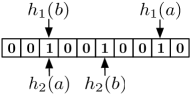
Figure 1: A Bloom filter with two hash functions

In order to check if an element $b$ of the universe $U$ belongs to the set $A$, all one has to do is check that the $k$ bits at positions $h_{1}(b),h_{2}(b),\ldots,h_{k}(b)$ are all set to 1. If at least one bit is set to 0, we are sure that $b$ does not belong to $A$. If all bits are set to 1, $b$ possibly belongs to $A$. There is always a probability that $b$ does not belong to $A$. In other words, there is a risk of false positives. Let us denote by $F_{\textrm{P}}$ the set of false positives, i.e., the elements that do not belong to $A$ (and thus that belong to $U-A$) and for which the Bloom filter gives a positive answer. The sets $U$, $A$, and $F_{\textrm{P}}$ are illustrated in Fig. 2. ($B$ is a subset of $F_{\textrm{P}}$ that will be introduced below.) In Fig. 2, $F_{\textrm{P}}$ is a circle surrounding $A$. (Note that $F_{\textrm{P}}$ is not a superset of $A$. It has been colored distinctly to indicate that it is disjoint from $A$.)

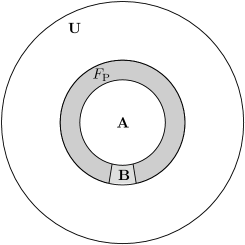
Figure 2: The false positives set

We define the false positive proportion $f_{\textrm{P}}$ as the ratio of the number of elements in $U-A$ that give a positive answer, to the total number of elements in $U-A$:

$$\begin{array}[]{ll}f_{\textrm{P}}&=~{}\frac{|F_{\textrm{P}}|}{|U-A|}\end{array}$$ (1)

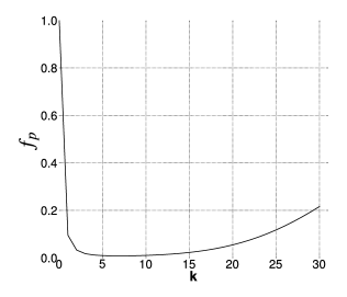
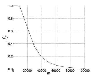
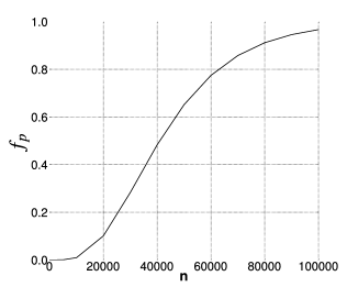
Figure 3: $f_{\textrm{P}}$ as a function of $k$, $m$ and $n$.

We can alternately define the false positive rate, as the probability that, for a given element that does not belong to the set $A$, the Bloom filter erroneously claims that the element is in the set. Note that if this probability exists (a hypothesis related to the ergodicity of the system that we assume here), it has the same value as the false positive proportion $f_{\textrm{P}}$. As a consequence, we will use the same notation for both parameters and also denote by $f_{\textrm{P}}$ the false positive rate. In order to calculate the false positive rate, most papers assume that all hash functions map each item in the universe to a random number uniformly over the range $\{1,\ldots,m\}$. As a consequence, the probability that a specific bit is set to 1 after the application of one hash function to one element of $A$ is $\frac{1}{m}$ and the probability that this specific bit is left to 0 is $1-\frac{1}{m}$. After all elements of $A$ are coded in the Bloom filter, the probability that a specific bit is always equal to 0 is

$$p_{0}~{}=~{}\left(1-\frac{1}{m}\right)^{kn}$$ (2)

As $m$ becomes large, $\frac{1}{m}$ is close to zero and $p_{0}$ can be approximated by

$$p_{0}~{}\approx~{}e^{-\frac{kn}{m}}$$ (3)

The probability that a specific bit is set to 1 can thus be expressed as

$$\begin{array}[]{ll}p_{1}&=~{}1-p_{0}\end{array}$$ (4)

The false positive rate can then be estimated by the probability that each of the $k$ array positions computed by the hash functions is 1. $f_{\textrm{P}}$ is then given by

$$\begin{array}[]{lll}f_{\textrm{P}}&=~{}p_{1}^{k}\\ &=~{}\left(1-\left(1-\frac{1}{m}\right)^{kn}\right)^{k}\\ &\approx~{}\left(1~{}-~{}e^{-\frac{kn}{m}}\right)^{k}\end{array}$$ (5)

The false positive rate $f_{\textrm{P}}$ is thus a function of three parameters: $n$, the size of subset $A$; $m$, the size of the filter; and $k$, the number of hash functions. Fig. 3 illustrates the variation of $f_{\textrm{P}}$ with respect to the three parameters individually (when the two others are held constant). Obviously, and as can be seen on these graphs, $f_{\textrm{P}}$ is a decreasing function of $m$ and an increasing function of $n$. Now, when $k$ varies (with $n$ and $m$ constant), $f_{\textrm{P}}$ first decreases, reaches a minimum and then increases. Indeed there are two contradicting factors: using more hash functions gives us more chances to find a $0$ bit for an element that is not a member of $A$, but using fewer hash functions increases the fraction of $0$ bits in the array. As stated, e.g., by Fan et al. [5], $f_{\textrm{P}}$ is minimized when

$$k~{}=~{}\frac{m\ln 2}{n}$$ (6)

for fixed $m$ and $n$. Indeed, the derivative of $f_{\textrm{P}}$ (estimated by eqn. 3) with respect to $k$ is $0$ when $k$ is given by eqn. 6, and it can further be shown that this is a global minimum.

Thus the minimum possible false positive rate for given values of $m$ and $n$ is given by eqn. 7. In practice, of course, $k$ must be an integer. As a consequence, the value furnished by eqn. 6 is rounded to the nearest integer and the resulting false positive rate will be somewhat higher than the optimal value given in eqn. 7.

$$\hat{f}_{\textrm{P}}~{}=~{}\left(\frac{1}{2}\right)^{\frac{m\ln 2}{n}}\approx~{}\left(0.6185\right)^{\frac{m}{n}}$$ (7)

Finally, it is important to emphasize that the absolute number of false positives is relative to the size of $U-A$ (and not directly to the size of $A$). This result seems surprising as the expression of $f_{\textrm{P}}$ depends on $n$, the size of $A$, and does not depend on $N$, the size of $U$. If we double the size of $U-A$ (and keep the size of $A$ constant) we also double the absolute number of false positives (and obviously the false positive rate is unchanged).

III Retouched Bloom Filters

As shown in Sec. II, there is a trade-off between the size of the Bloom filter and the probability of a false positive. For a given $n$, even by optimally choosing the number of hash functions, the only way to reduce the false positive rate in standard Bloom filters is to increase the size $m$ of the bit vector. Unfortunately, although this implies a gain in terms of a reduced false positive rate, it also implies a loss in terms of increased memory usage. Bandwidth usage becomes a constraint that must be minimized when Bloom filters are transmitted in the network.

III-A Bit Clearing

In this paper, we introduce an extension to the Bloom filter, referred to as the retouched Bloom filter (RBF). The RBF makes standard Bloom filters more flexible by allowing selected false positives to be traded off against random false negatives. False negatives do not arise at all in the standard case. The idea behind the RBF is to remove a certain number of these selected false positives by resetting individually chosen bits in the vector $v$. We call this process the bit clearing process. Resetting a given bit to 0 not only has the effect of removing a certain number of false positives, but also generates false negatives. Indeed, any element $a\in A$ such that (at least) one of the $k$ bits at positions $h_{1}(a),h_{2}(a),\ldots,h_{k}(a)$ has been reset to 0, now triggers a negative answer. Element $a$ thus becomes a false negative.

To summarize, the bit clearing process has the effects of decreasing the number of false positives and of generating a number of false negatives. Let us use the labels $F_{\textrm{P}}^{\prime}$ and $F_{\textrm{N}}^{\prime}$ to describe the sets of false positives and false negatives after the bit clearing process. The sets $F_{\textrm{P}}^{\prime}$ and $F_{\textrm{N}}^{\prime}$ are illustrated in Fig. 4.

Figure 4: False positive and false negative sets after the selective clearing process

After the bit clearing process, the false positive and false negative proportions are given by

$$\begin{array}[]{ll}f_{\textrm{P}}^{\prime}&=~{}\frac{|F_{\textrm{P}}^{\prime}|}{|U-A|}\end{array}$$ (8)

$$\begin{array}[]{ll}f_{\textrm{N}}^{\prime}&=~{}\frac{|F_{\textrm{N}}^{\prime}|}{|A|}\end{array}$$ (9)

Obviously, the false positive proportion has decreased (as $F_{\textrm{P}}^{\prime}$ is smaller than $F_{\textrm{P}}$) and the false negative proportion has increased (as it was zero before the clearing). We can measure the benefit of the bit clearing process by introducing $\Delta f_{\textrm{P}}$, the proportion of false positives removed by the bit clearing process, and $\Delta f_{\textrm{N}}$, the proportion of false negatives generated by the bit clearing process:

$$\Delta f_{\textrm{P}}~{}=~{}\frac{|F_{\textrm{P}}|-|F_{\textrm{P}}^{\prime}|}{|F_{\textrm{P}}|}=\frac{f_{\textrm{P}}-f_{\textrm{P}}^{\prime}}{f_{\textrm{P}}}$$ (10)

$$\Delta f_{\textrm{N}}~{}=~{}\frac{|F_{\textrm{N}}^{\prime}|}{|A|}=f_{\textrm{N}}^{\prime}$$ (11)

We, finally, define $\chi$ as the ratio between the proportion of false positives removed and the proportion of false negatives generated:

$$\chi~{}=~{}\frac{\Delta f_{\textrm{P}}}{\Delta f_{\textrm{N}}}$$ (12)

$\chi$ is the main metric we introduce in this paper in order to evaluate the RBF. If $\chi$ is greater than 1, it means that the proportion of false positives removed is higher than the proportion of false negatives generated.

III-B Randomized Bit Clearing

In this section, we analytically study the effect of randomly resetting bits in the Bloom filter, whether these bits correspond to false positives or not. We call this process the randomized bit clearing process. In Sec. IV, we discuss more sophisticated approaches to choosing the bits that should be cleared. However, performing random clearing in the Bloom filter enables us to derive analytical results concerning the consequences of the clearing process. In addition to providing a formal derivation of the benefit of RBFs, it also gives a lower bound on the performance of any smarter selective clearing approach (such as those developed in Sec. IV).

We again assume that all hash functions map each element of the universe $U$ to a random number uniformly over the range $\{1,\ldots,m\}$. Once the $n$ elements of $A$ have been coded in the Bloom filter, there is a probability $p_{0}$ for a given bit in $v$ to be $0$ and a probability $p_{1}$ for it to be $1$. As a consequence, there is an average number of $p_{1}m$ bits set to $1$ in $v$. Let us study the effect of resetting to $0$ a randomly chosen bit in $v$. Each of the $p_{1}m$ bits set to $1$ in $v$ has a probability $\frac{1}{p_{1}m}$ of being reset and a probability $1-\frac{1}{p_{1}m}$ of being left at $1$.

The first consequence of resetting a bit to $0$ is to remove a certain number of false positives. If we consider a given false positive $x\in F_{\textrm{P}}$, after the reset it will not result in a positive test any more if the bit that has been reset belongs to one of the $k$ positions $h_{1}(x),h_{2}(x),\ldots,h_{k}(x)$. Conversely, if none of the $k$ positions have been reset, $x$ remains a false positive. The probability of this latter event is

$$r_{1}~{}=~{}\left(1-\frac{1}{p_{1}m}\right)^{k}$$ (13)

As a consequence, after the reset of one bit in $v$, the false positive rate decreases from $f_{\textrm{P}}$ (given by eqn. 5) to $f_{\textrm{P}}^{\prime}=f_{\textrm{P}}r_{\textrm{1}}$. The proportion of false positives that have been eliminated by the resetting of a randomly chosen bit in $v$ is thus equal to $1-r_{1}$:

$$\Delta f_{\textrm{P}}~{}=~{}1-r_{1}$$ (14)

The second consequence of resetting a bit to $0$ is the generation of a certain number of false negatives. If we consider a given element $a\in A$, after the reset it will result in a negative test if the bit that has been reset in $v$ belongs to one of the $k$ positions $h_{1}(a),h_{2}(a),\ldots,h_{k}(a)$. Conversely, if none of the $k$ positions have been reset, the test on $a$ remains positive. Obviously, the probability that a given element in $A$ becomes a false negative is given by $1-r_{1}$ (the same reasoning holds):

$$\Delta f_{\textrm{N}}~{}=~{}1-r_{1}$$ (15)

We have demonstrated that resetting one bit to $0$ in $v$ has the effect of eliminating the same proportion of false positives as the proportion of false negatives generated. As a result, $\chi=1$. It is however important to note that the proportion of false positives that are eliminated is relative to the size of the set of false positives (which in turns is relative to the size of $U-A$, thanks to eqn. 5) whereas the proportion of false negatives generated is relative to the size of $A$. As we assume that $U-A$ is much bigger than $A$ (actually if $|F_{\textrm{P}}|>|A|$), resetting a bit to $0$ in $v$ can eliminate many more false positives than the number of false negatives generated.

It is easy to extend the demonstration to the reset of $s$ bits and see that it eliminates a proportion $1-r_{s}$ of false positives and generates the same proportion of false negatives, where $r_{s}$ is given by

$$r_{s}~{}=~{}\left(1-\frac{s}{p_{1}m}\right)^{k}$$ (16)

As a consequence, any random clearing of bits in the Bloom vector $v$ has the effect of maintaining the ratio $\chi$ equal to $1$.

IV Selective Clearing

Sec. III introduced the idea of randomized bit clearing and analytically studied the effect of randomly resetting $s$ bits of $v$, whether these bits correspond to false positives or not. We showed that it has the effect of maintaining the ratio $\chi$ equal to 1. In this section, we refine the idea of randomized bit clearing by focusing on bits corresponding to elements that trigger false positives. We call this process selective clearing.

As described in Sec. II, in Bloom filters (and also in RBFs), some elements in $U-A$ will trigger false positives, forming the set $F_{\textrm{P}}$. However, in practice, it is likely that not all false positives will be encountered. To illustrate this assertion, let us assume that the universe $U$ consists of the whole IPv4 addresses range. To build the Bloom filter or the RBF, we define $k$ hash functions based on a 32 bit string. The subset $A$ to record in the filter is a small portion of the IPv4 address range. Not all false positives will be encountered in practice because a significant portion of the IPv4 addresses in $F_{\textrm{P}}$ have not been assigned.

We record the false positives encountered in practice in a set called $B$, with $B\subseteq F_{\textrm{P}}$ (see Fig. 2). Elements in $B$ are false positives that we label as troublesome keys, as they generate, when presented as keys to the Bloom filter’s hash functions, false positives that are liable to be encountered in practice. We would like to eliminate the elements of $B$ from the filter.

In the following sections, we explore several algorithms for performing selective clearing (Sec. IV-A). We then evaluate and compare the performance of these algorithms using theorical analysis (Sec. IV-B) and simulation analysis (Sec. IV-C).

IV-A Algorithms

In this section, we propose four different algorithms that allow one to remove the false positives belonging to $B$. All of these algorithms are simple to implement and deploy. We first present an algorithm that does not require any intelligence in selective clearing. Next, we propose refined algorithms that take into account the risk of false negatives. With these algorithms, we show how to trade-off false positives for false negatives.

The first algorithm is called Random Selection. The main idea is, for each troublesome key to remove, to randomly select a bit amongst the $k$ available to reset. The main interest of the Random Selection algorithm is its extreme computational simplicity: no effort has to go into selecting a bit to clear. Random Selection differs from random clearing (see Sec. III) by focusing on a set of troublesome keys to remove, $B$, and not by resetting randomly any bit in $v$, whether it corresponds to a false positive or not. Random Selection is formally defined in Algorithm 1.

Algorithm 1 Random Selection

1:$v$, the bit vector.

2:$v$ updated, if needed.

3:

4:procedure RandomSelection($B$)

5:

6:for all $b_{i}\in B$ do

7:

8:if MembershipTest($b_{i}$, $v$) then

9:

10:index $\leftarrow$ Random($h_{1}(b_{i})$, …, $h_{k}(b_{i})$)

11:

12:$v$[index] $\leftarrow$ 0

13:end if

14:end for

15:end procedure

Recall that $B$ is the set of troublesome keys to remove. This set can contain from only one element to the whole set of false positives. Before removing a false positive element, we make sure that this element is still falsely recorded in the RBF, as it could have been removed previously. Indeed, due to collisions that may occur between hashed keys in the bit vector, as shown in Fig. 1, one of the $k$ hashed bit positions of the element to remove may have been previously reset. Algorithm 1 assumes that a function Random is defined and returns a value randomly chosen amongst its uniformly distributed arguments. The algorithm also assumes that the function MembershipTest is defined. It takes two arguments: the key to be tested and the bit vector. This function returns true if the element is recorded in the bit vector (i.e., all the $k$ positions corresponding to the hash functions are set to 1). It returns false otherwise.

The second algorithm we propose is called Minimum FN Selection. The idea is to minimize the false negatives generated by each selective clearing. For each troublesome key to remove that was not previously cleared, we choose amongst the $k$ bit positions the one that we estimate will generate the minimum number of false negatives. This minimum is given by the MinIndex procedure in Algorithm 2. This can be achieved by maintaining locally a counting vector, $v_{A}$, storing in each vector position the quantity of elements recorded. This algorithm effectively takes into account the possibility of collisions in the bit vector between hashed keys of elements belonging to $A$. Minimum FN Selection is formally defined in Algorithm 2.

For purposes of algorithmic simplicity, we do not entirely update the counting vector with each iteration. The cost comes in terms of an over-estimation, for the heuristic, in assessing the number of false negatives that it introduces in any given iteration. This over-estimation grows as the algorithm progresses. We are currently studying ways to efficiently adjust for this over-estimation. Sec. V will discuss more complex selective clearing algorithms that update, at each step, the counting vector.

Algorithm 2 Minimum FN Selection

1:$v$, the bit vector and $v_{A}$, the counting vector.

2:$v$ and $v_{A}$ updated, if needed.

3:

4:procedure MinimumFNSelection($B$)

5:

6:CreateCV($A$)

7:

8:for all $b_{i}\in B$ do

9:

10:if MembershipTest($b_{i}$, $v$) then

11:

12:index $\leftarrow$ MinIndex($b_{i}$)

13:

14:$v$[index] $\leftarrow$ 0

15:

16:$v_{A}$[index] $\leftarrow$ 0

17:end if

18:end for

19:end procedure

20:

21:

22:

23:procedure CreateCV($A$)

24:

25:for all $a_{i}\in A$ do

26:

27:for $j=1\mathrm{\ to\ }k$ do

28:

29:$v_{A}$[$h_{j}(a_{i})$]++

30:end for

31:end for

32:end procedure

The third selective clearing mechanism is called Maximum FP Selection. In this case, we try to maximize the quantity of false positives to remove. For each troublesome key to remove that was not previously deleted, we choose amongst the $k$ bit positions the one we estimate to allow removal of the largest number of false positives, the position of which is given by the MaxIndex function in Algorithm 3. In the fashion of the Minimum FN Selection algorithm, this is achieved by maintaining a counting vector, $v_{B}$, storing in each vector position the quantity of false positive elements recorded. For each false positive element, we choose the bit corresponding to the largest number of false positives recorded. This algorithm considers as an opportunity the risk of collisions in the bit vector between hashed keys of elements generating false positives. Maximum FP Selection is formally described in Algorithm 3.

Algorithm 3 Maximum FP Selection

1:$v$, the bit vector and $v_{B}$, the counting vector.

2:$v$ and $v_{B}$ updated, if needed.

3:

4:procedure MaximumFP($B$)

5:

6:CreateFV($B$)

7:

8:for all $b_{i}\in B$ do

9:

10:if MembershipTest($b_{i}$, $v$) then

11:

12:index $\leftarrow$ MaxIndex($b_{i}$)

13:

14:$v$[index] $\leftarrow$ 0

15:

16:$v_{B}$[index] $\leftarrow$ 0

17:end if

18:end for

19:end procedure

20:

21:

22:

23:procedure CreateFV($B$)

24:

25:for all $b_{i}\in B$ do

26:

27:for $j=1\mathrm{\ to\ }k$ do

28:

29:$v_{B}$[$h_{j}(b_{i})$]++

30:end for

31:end for

32:end procedure

Finally, we propose a selective clearing mechanism called Ratio Selection. The idea is to combine Minimum FN Selection and Maximum FP Selection into a single algorithm. Ratio Selection provides an approach in which we try to minimize the false negatives generated while maximizing the false positives removed. Ratio Selection therefore takes into account the risk of collision between hashed keys of elements belonging to $A$ and hashed keys of elements belonging to $B$. It is achieved by maintaining a ratio vector, $r$, in which each position is the ratio between $v_{A}$ and $v_{B}$. For each troublesome key that was not previously cleared, we choose the index where the ratio is the minimum amongst the $k$ ones. This index is given by the MinRatio function in Algorithm 4. Ratio Selection is defined in Algorithm 4. This algorithm makes use of the CreateCV and CreateFV functions previously defined for Algorithms 2 and 3.

Algorithm 4 Ratio Selection

1:$v$, the bit vector, $v_{B}$ and $v_{A}$, the counting vectors and $r$, the ratio vector.

2:$v$, $v_{A}$, $v_{B}$ and $r$ updated, if needed.

3:

4:procedure Ratio($B$)

5:

6:CreateCV($A$)

7:

8:CreateFV($B$)

9:

10:ComputeRatio()

11:

12:for all $b_{i}\in B$ do

13:

14:if MembershipTest($b_{i}$, $v$) then

15:

16:index $\leftarrow$ MinRatio($b_{i}$)

17:

18:$v$[index] $\leftarrow$ 0

19:

20:$v_{A}$[index] $\leftarrow$ 0

21:

22:$v_{B}$[index] $\leftarrow$ 0

23:

24:$r$[index] $\leftarrow$ 0

25:end if

26:end for

27:end procedure

28:

29:

30:

31:procedure ComputeRatio

32:

33:for $i=1\mathrm{\ to\ }m$ do

34:

35:if $v$[i] $\wedge$ $v_{B}[i]>0$ then

36:

37:$r$[i] $\leftarrow$ $\frac{v_{A}[i]}{v_{B}[i]}$

38:end if

39:end for

40:end procedure

IV-B Theorical Analysis

IV-B1 Algorithmic Complexity

Lemma 1

The algorithmic complexity of the Random Selection algorithm is $O(k\times|B|)$.

Proof:

Before going into details of the Random Selection algorithm, let us first have a look at the MembershipTest procedure. This procedure takes two arguments: $x_{i}$, an element belonging to $|B|$ and $v$, the bit vector. The MembershipTest procedure aims at determining whether the element $x_{i}$ is recorded in the bit vector $v$, or not. Therefore, as explained in Sec. II, the MembershipTest procedure checks if the $k$ bits at positions $h_{1}(b),h_{2}(b),\ldots,h_{k}(b)$ are all set to 1. As a consequence, the algorithmic complexity of the MembershipTest is $O(k)$.

Now, let us consider the Random Selection algorithm in its entirety. Random Selection browses all elements belonging to $B$. And for each element in $B$, Random Selection calls the MembershipTest procedure. Therefore, the MembershipTest procedure is called $|B|$ times.

Consequently, the algorithmic complexity of the Random Selection is $O(k\times|B|)$. ∎

Lemma 2

The running time of the Minimum FN Selection algorithm is $O(k\times(|A|+|B|))$.

Proof:

We first have a look at the CreateCV procedure. CreateCV aims at creating the counting vector $v_{A}$ that indicates, for each cell, the number of element recorded in the corresponding cell of the bit vector $v$. Therefore, this procedure browses all elements belonging to $A$ and, for each element, increments $k$ counters, where $k$ gives the number of hash functions used. Consequently, the algorithmic complexity of the CreateCV procedure is $O(k\times|A|)$.

After returning from the CreateCV procedure call, the Minimum FN Selection algorithm browses all elements belonging to $B$ and, for each element, calls MembershipTest. If the membership test returns true, then the MinIndex procedure is called. This procedure aims at determining the bit vector index that returns the minimum value among $k$ available. The algorithmic complexity is thus $O(k)$.

Until now, the complexity of Minimum FN Selection is $O(\max(k\times|A|,2k\times|B|))$. The term $2k$ can be reduced to $k$. Finally, it is easy to show that $O(k\times\max(|A|,|B|))$ is equivalent to $O(k\times(|A|+|B|))$. ∎

Lemma 3

The running time of the Maximum FP Selection algorithm is $O(k\times|B|)$.

Proof:

Let us first consider the CreateFV procedure. This aims at creating the counting vector $v_{B}$ that indicates, for each cell, the number of false positives recorded in the corresponding cell of the bit vector $v$. Therefore, this procedure browses all elements belonging to $B$ and, for each element, increments $k$ counters, where $k$ gives the number of hash functions used. Consequently, the algorithmic complexity of the CreateFV procedure is $O(k\times|B|)$.

After returning from the CreateFV procedure call, the Maximum FP Selection algorithm browses all elements belonging to $B$ and, for each element, calls MembershipTest. If the membership test returns true, then the MaxIndex procedure is called. This procedure aims at determining the bit vector index that returns the maximum value among $k$ available. The algorithmic complexity is thus $O(k)$.

Until now, the complexity of Maximum FP Selection is $O(2\times(k\times|B|))$. The multiplicative factor $2$ is negligible. Consequently, the algorithmic complexity of the Maximum FP Selection algorithm is $O(k\times|B|)$. ∎

Lemma 4

The running time of the Ratio Selection algorithm is $O(k\times(|A|+|B|)+m)$.

Proof:

As explained above, the complexity of CreateCV is $O(k\times|A|)$ and CreateFV is $O(k\times|B|)$. After calling CreateCV and CreateFV, the Ratio Selection algorithm calls the Ratio procedure that aims at creating the ratio of $v_{A}$ to $v_{B}$. The complexity of Ratio is $O(m)$ as it must browses all vector cells.

The rest of Ratio Selection behaves the same way as Minimum FN Selection and Maximum FP Selection, i.e., it browses all elements belonging to $B$, performs the membership test and, if needed, selects the minimum value among $k$ available. Therefore, the complexity is $O(k\times(|A|+|B|))$ to which we add the cost associated to the ComputeRatio procedure, i.e. $O(m)$.

Consequently, the algorithmic complexity is $O(k\times(|A|+|B|)+m)$. ∎

IV-B2 Spatial Complexity

Lemma 5

The spatial complexity of the Random Selection algorithm is $O(m+|B|)$

Proof:

The Random Selection algorithm makes use of two data structures: $v$, the bit vector required by the Bloom filters, and $B$, the set of troublesome keys to remove from the Bloom filter. The vector $v$ is $m$ bit long. Therefore, the spatial complexity of the Random Selection algorithm is $O(m+|B|)$. ∎

Lemma 6

The spatial complexity of the Minimum FN Selection algorithm is $O(cm+|B|)$

Proof:

The Minimum FN Selection algorithm makes use of three data structures: $v$, the $m$ bit vector, $B$, the set of troublesome keys to remove from the Bloom filter and $v_{A}$, the counting vector. $v_{A}$ is $m$ cells long and each cell contains $c$ bits needed by the counter. Therefore, the spatial complexity of the Minimum FN Selection algorithm is $O(cm+|B|)$. ∎

Lemma 7

The spatial complexity of the Maximum FP Selection algorithm is $O(cm+|B|)$.

Proof:

The Maximum FP Selection algorithm makes use of three data structures: $v$, the $m$ bit vector, $B$, the set of troublesome keys to remove from the Bloom filter and $v_{B}$, the counting vector. $v_{B}$ is $m$ cells long and each cell contains $c$ bits needed by the counter. Therefore, the spatial complexity of the Maximum FP Selection algorithm is $O(cm+|B|)$. ∎

Lemma 8

The spatial complexity of the Ratio Selection algorithm is $O(cm+dm+|B|)$.

Proof:

The Ratio Selection algorithm makes use of four data structures: $v$, the $m$ bit vector, $B$, the set of troublesome keys to remove from the Bloom filter, $v_{A}$, the counting vector of elements truly recorded in $v$, $v_{B}$, the counting vector of false positives recorded in $v$ and $r$, the ratio vector. $r$ is $m$ cells long and each cell contains $d$ bits needed by the counter. Note that $d$ is greater than $c$ as $r$ records ratios. Therefore, the spatial complexity Ratio algorithm is $O(cm+dm+|B|)$. ∎

IV-C Simulation Analysis

IV-C1 Methodology

We conducted an experiment with a universe $U$ of 2,000,000 elements ($N=2,000,000$). These elements, for the sake of simplicity, were integers belonging to the range [0; 1,999,9999]. The subset $A$ that we wanted to summarize in the Bloom filter contains 10,000 different elements ($n=10,000$) randomly chosen from the universe $U$. Bloom’s paper [1] states that $|U|$ must be much greater than $|A|$, without specifying a precise scale.

The bit vector $v$ we used for simulations is 100,000 bits long ($m=100,000$), ten times bigger than $|A|$. The RBF used five different and independent hash functions ($k=5$). Hashing was emulated with random numbers. We simulated randomness with the Mersenne Twister MT19937 pseudo-random number generator [6]. Using five hash functions and a bit vector ten times bigger than $n$ is advised by Fan et al. [5]. This permits a good trade-off between membership query accuracy, i.e., a low false positive rate of 0.0094 when estimated with eqn. 5, memory usage and computation time. As mentioned earlier in this paper (see Sec. II), the false positive rate may be decreased by increasing the bit vector size but it leads to a lower compression level.

For our experiment, we defined the ratio of troublesome keys compared to the entire set of false positives as

$$\beta~{}=~{}\frac{|B|}{|F_{P}|}$$ (17)

We considered the following values of $\beta$: 1%, 2%, 5%, 10%, 25%, 50%, 75% and 100%. When $\beta=100$%, it means that $B=F_{\textrm{P}}$ and we want to remove all the false positives.

Each data point in the plots and tables represents the mean value over fifteen runs of the experiment, each run using a new $A$, $F_{\textrm{P}}$, $B$, and RBF. We determined 95% confidence intervals for the mean based on the Student $t$ distribution.

We performed the experiment as follows: we first created the universe $U$ and randomly affected 10,000 of its elements to $A$. We next built $F_{\textrm{P}}$ by applying the following scheme. Rather than using eqn. 5 to compute the false positive rate and then creating $F_{\textrm{P}}$ by randomly affecting positions in $v$ for the false positive elements, we preferred to experimentally compute the false positives. We queried the RBF with a membership test for each element belonging to $U-A$. False positives were the elements that belong to the Bloom filter but not to $A$. We kept track of them in a set called $F_{\textrm{P}}$. This process seemed to us more realistic because we evaluated the real quantity of false positive elements in our data set. $B$ was then constructed by randomly selecting a certain quantity of elements in $F_{\textrm{P}}$, the quantity corresponding to the desired cardinality of $B$. We next removed all troublesome keys from $B$ by using one of the selective clearing algorithms, as explained in Sec. IV-A. We then built $F_{\textrm{N}}^{\prime}$, the false negative set, by testing all elements in $A$ and adding to $F_{\textrm{N}}^{\prime}$ all elements that no longer belong to $A$. We also determined $F_{\textrm{P}}^{\prime}$, the false positive set after removing the set of troublesome keys $B$.

IV-C2 Results

	$|B|$		$|B^{\prime}|$		$|B|+|B^{\prime}|$		$|A^{\prime}|$
1%	188	$\pm 1.31$	434	$\pm 13.74$	622	$\pm 13.84$	231	$\pm 3.01$
2%	375	$\pm 1.84$	842	$\pm 21.84$	1217	$\pm 22.85$	450	$\pm 7.75$
5%	932	$\pm 9.94$	1934	$\pm 37.83$	2826	$\pm 46.21$	1070	$\pm 10.05$
10%	1872	$\pm 17.22$	3306	$\pm 67.83$	5178	$\pm 83.27$	1954	$\pm 20.02$
25%	4692	$\pm 26.11$	5441	$\pm 61.11$	10133	$\pm 83.45$	3858	$\pm 21.14$
50%	9396	$\pm 78.88$	5324	$\pm 67.09$	14720	$\pm 143.22$	5684	$\pm 36.78$
75%	14063	$\pm 109.61$	3151	$\pm 36.92$	17214	$\pm 144.08$	6715	$\pm 30.44$
100%	18806	$\pm 157.31$	0		18806	$\pm 157.31$	7367	$\pm 23.93$

TABLE I: Random Selection

	$|B|$		$|B^{\prime}|$		$|B|+|B^{\prime}|$		$|A^{\prime}|$
1%	188	$\pm 1.09$	431	$\pm 15.27$	619	$\pm 16.11$	183	$\pm 1.82$
2%	377	$\pm 2.75$	854	$\pm 18.14$	1231	$\pm 19.39$	362	$\pm 3.77$
5%	939	$\pm 7.67$	1942	$\pm 28.77$	2881	$\pm 33.57$	857	$\pm 9.82$
10%	1877	$\pm 12.79$	3303	$\pm 65.26$	5180	$\pm 76.46$	1577	$\pm 14.92$
25%	4667	$\pm 35.36$	5338	$\pm 72.65$	10045	$\pm 105.28$	3143	$\pm 19.83$
50%	9365	$\pm 44.51$	5330	$\pm 52.09$	14695	$\pm 92.01$	4754	$\pm 24.27$
75%	14039	$\pm 85.94$	3128	$\pm 37.98$	17167	$\pm 119.53$	5710	$\pm 21.64$
100%	18705	$\pm 173.76$	0		18705	$\pm 173.76$	6407	$\pm 36.02$

TABLE II: Minimum FN Selection

	$|B|$		$|B^{\prime}|$		$|B|+|B^{\prime}|$		$|A^{\prime}|$
1%	187	$\pm 0.93$	769	$\pm 9.97$	956	$\pm 10.28$	226	$\pm 5.11$
2%	375	$\pm 1.82$	1458	$\pm 19.33$	1833	$\pm 20.05$	447	$\pm 8.96$
5%	935	$\pm 6.36$	3154	$\pm 52.89$	4089	$\pm 58.78$	1025	$\pm 12.08$
10%	1882	$\pm 16.55$	5188	$\pm 74.87$	7070	$\pm 89.71$	1838	$\pm 20.53$
25%	4697	$\pm 34.52$	7466	$\pm 85.07$	12163	$\pm 114.96$	3420	$\pm 28.49$
50%	9396	$\pm 86.71$	6605	$\pm 98.04$	16001	$\pm 182.14$	4870	$\pm 29.84$
75%	14032	$\pm 99.42$	3670	$\pm 28.61$	17702	$\pm 125.24$	5674	$\pm 26.34$
100%	18664	$\pm 138.13$	0		18664	$\pm 138.13$	6202	$\pm 22.09$

TABLE III: Maximum FP Selection

	$|B|$		$|B^{\prime}|$		$|B|+|B^{\prime}|$		$|A^{\prime}|$
1%	188	$\pm 1.51$	735	$\pm 13.89$	923	$\pm 14.63$	188	$\pm 1.58$
2%	374	$\pm 3.25$	1372	$\pm 20.05$	1746	$\pm 30.58$	363	$\pm 4.01$
5%	939	$\pm 6.92$	3035	$\pm 40.83$	3974	$\pm 45.43$	844	$\pm 5.73$
10%	1863	$\pm 13.95$	4860	$\pm 67.65$	6723	$\pm 78.71$	1498	$\pm 13.71$
25%	4703	$\pm 28.72$	7261	$\pm 68.39$	11964	$\pm 94.59$	2895	$\pm 15.99$
50%	9394	$\pm 80.17$	6444	$\pm 70.86$	15838	$\pm 149.01$	4229	$\pm 25.95$
75%	14057	$\pm 126.61$	3625	$\pm 38.28$	17682	$\pm 162.64$	5021	$\pm 27.54$
100%	18683	$\pm 151.08$	0		18683	$\pm 151.08$	5581	$\pm 24.08$

TABLE IV: Ratio Selection

Table I to IV present performance results for the selective clearing algorithms proposed in Sec. IV-A. The mean over the fifteen run and the confidence intervals are shown. The column $|B|$ gives the number of troublesome keys to remove. The column $|B^{\prime}|$ gives an idea of the side effect of performing selective clearing, in terms of additional false positive keys removed. The column $|B+B^{\prime}|$ shows the total number of false positive removed. Finally, the last column, $|A^{\prime}|$, illustrates the quantity of keys that become false negatives after selective clearing.

Looking first at the side effects (i.e., column $|B^{\prime}|$), we see that removing troublesome keys in $B$ has the consequence of removing other false positives. Maximum FP Selection (Table II) and Ratio Selection (Table IV) have a larger side effect compared to the two other selective clearing algorithms. We further note that the total amount of false positives removed from the filter (column $|B+B^{\prime}|$) is larger than the quantity of false negative generated (column $|A^{\prime}|$). This was expected, as explained in Sec. III-B.

Looking now at the quantity of false negative generated, one can see that Minimum FN Selection (Table II) and Ratio Selection generates fewer false negatives than Maximum FP Selection and Random Selection.

Consequently, from these preliminary results, one concludes that the Ratio Selection algorithm provides better performance. In the rest of this section, we will see if this conclusion is still valid when comparing the four selective algorithms in terms of the number of reset bits required to remove troublesome keys in $B$ and in terms of the $\chi$ metric.

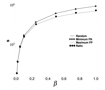
Figure 5: Number of bits reset

Fig. 5 compares the four algorithms in terms of the number $s$ of reset bits required to remove troublesome keys in $B$. The horizontal axis gives $\beta$ and the vertical axis, in log scale, gives $s$. The confidence intervals are plotted but they are too tight to appear clearly.

We see that Random Selection and Minimum FN Selection need to work more, in terms of number of bits to reset, when $\beta$ grows, compared to Maximum FP Selection and Ratio Selection. In addition, we note that the Ratio Selection algorithm needs to reset somewhat more bits than Maximum FP Selection (the difference is too tight to be clearly visible on the plots).

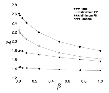
Figure 6: Effect on $\chi$

Fig. 6 evaluates the performance of the four algorithms. It plots $\beta$ on the horizontal axis and $\chi$ on the vertical axis. Again, the confidence intervals are plotted but they are generally too tight to be visible.

We first note that, whatever the algorithm considered, the $\chi$ ratio is always above 1, meaning that the advantages of removing false positives overcome the drawbacks of generating false negatives, if these errors are considered equally grave. Thus, as expected, performing selective clearing provides better results than randomized bit clearing. Ratio Selection does best, followed by Maximum FP, Minimum FN, and Ratio Selection.

The $\chi$ ratio for Random Selection does not vary much with $\beta$ compared to the three other algorithms. For instance, the $\chi$ ratio for Ratio Selection is decreased by 31.3% between $\beta$=1% and $\beta$=100%.

To summarize, one can say that, when using RBF, one can reliably get a $\chi$ above 1.4, even when using a simple selective clearing algorithm, such as Random Selection. Applying a more efficient algorithm, such as Ratio Selection, allows one to get a $\chi$ above 1.8. Such $\chi$ values mean that the proportion of false positives removed is higher than the proportion of false negatives generated.

In this section, we provided and evaluated four simple selective algorithms. We showed that two algorithms, Maximum FP Selection and Ratio Selection, are more efficient in terms of number of bits to clear in the filter. Among these two algorithms, we saw that Ratio Selection provides better results, in terms of the $\chi$ ratio.

V Improving Selective Clearing

Sec. IV discussed four selective clearing algorithms. Most of these algorithms simplifies the selective clearing process by not updating the counting vectors when a particular troublesome key is removed from the bit vector. This leads to an over-estimation of the quantity of false negatives generated at each step, as well as a sub-estimation of the amount of false positives removed at each step.

This section investigates improved selective clearing algorithms that keep up to date the quantity of false negatives removed and false positives removed at each step of the algorithms.

Sec. V-A discusses three improved selective algorithms; Sec. V-B proposes a theorical analysis of the improved selective algorithms; finally, Sec. V-C compares the performances of the improved selective algorithms with the standard algorithms introduced in Sec. IV.

V-A Algorithms

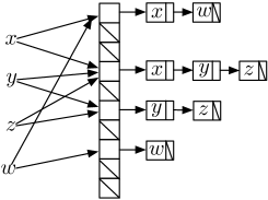
Figure 7: Example of an ElementList vector

Our improved selective clearing algorithms, instead of using counting vectors, make use of a particular data structure illustrated in Fig. 7. We call such a data structure ElementList vector. This is somewhat similar to the fast hash tables developed by Song et al. [7].

The vector has the same length than the bit vector. It contains thus $m$ cells. Each cell is a pointer to a list of elements recorded in that position in the bit vector. These elements, depending on the selective clearing algorithm, can belong to $A$ or $B$.

The first algorithm is an improvement to the Minimum FN Selection algorithm, called Improved Minimum FN Selection. Recall that Minimum FN Selection aims, for each troublesome key to remove, at selecting a bit amongst the $k$ available that will generate the minimum number of false negatives. In the fashion of Minimum FN Selection, the minimum is given by the MinIndex procedure in Algorithm 5. Instead of maintaining locally a counting vector, as done with the standard Minimum FN Selection algorithm, an ElementList vector, $v_{A}$, as illustrated in Fig. 7, is now used. Each cell of $v_{A}$ contains the list of elements belonging to $A$ that are recorded in the corresponding cell of $v$, the bit vector. When the minimum index has been returned by MinIndex, the Improved Minimum FN Selection algorithm call the BitClearing procedure that will remove from $v_{A}$ all the elements recorded in this minimum index. This was introduced in order to tackle the over-estimation of the standard Minimum FN Selection where the counting vector was not entirely updated at each step of the algorithm. Improved Minimum FN Selection is formally defined in Algorithm 5.

Algorithm 5 Improved Minimum FN Selection

1:$v$, the bit vector and $v_{A}$, the element vector.

2:$v$ and $v_{A}$ updated, if needed.

3:

4:procedure MinimumFNSelection($B$)

5:

6:CreateCV($A$)

7:

8:for all $b_{i}\in B$ do

9:

10:if MembershipTest($b_{i}$, $v$) then

11:

12:index $\leftarrow$ MinIndex($b_{i}$)

13:

14:BitClearing($v_{A}$, index)

15:

16:$v$[index] $\leftarrow$ 0

17:end if

18:end for

19:end procedure

20:

21:

22:

23:procedure CreateCV($A$)

24:

25:for all $a_{i}\in A$ do

26:

27:for $j=1\mathrm{\ to\ }k$ do

28:

29:$v_{A}$[$h_{j}(a_{i})$].add($a_{i}$)

30:end for

31:end for

32:end procedure

33:

34:

35:

36:procedure BitClearing($\nu$, index)

37:

38:ElementList el = $\nu$.get(index)

39:

40:for all $x_{i}\in el$ do

41:

42:Remove($x_{i}$, $\nu$)$\triangleright$ remove all occurrences of element $x_{i}$ from $\nu$

43:end for

44:end procedure

Note that the MembershipTest procedure is identical to the one introduced in Sec. IV-A.

The second improved selective clearing algorithm is an improvement to the Maximum FP Selection algorithm and is called Improved Maximum FP Selection. The standard Maximum FP Selection algorithm, defined in Algorithm 3, aims at removing the maximum quantity of troublesome false positives at each step of the algorithm. Improved Maximum FP Selection behaves mainly in the same way, except it makes use of an element vector, $v_{B}$, instead of a counting vector. When the maximum index is found by the MaxIndex procedure, the BitClearing procedure is called in order to maintain $v_{B}$ up-to-date. Improved Maximum FP Selection is formally defined in Algorithm 6.

Algorithm 6 Improved Maximum FP Selection

1:$v$, the bit vector and $v_{B}$, the element vector.

2:$v$ and $v_{\textrm{B}}$ updated, if needed.

3:

4:procedure MaximumFP($B$)

5:

6:CreateFV($B$)

7:

8:for all $b_{i}\in B$ do

9:

10:if MembershipTest($b_{i}$, $v$) then

11:

12:index $\leftarrow$ MaxIndex($b_{i}$)

13:

14:BitClearing($v_{B}$, index)

15:

16:$v$[index] $\leftarrow$ 0

17:end if

18:end for

19:end procedure

20:

21:

22:

23:procedure CreateFV($B$)

24:

25:for all $b_{i}\in B$ do

26:

27:for $j=1\mathrm{\ to\ }k$ do

28:

29:$v_{B}$[$h_{j}(b_{i})$].add($b_{i}$)

30:end for

31:end for

32:end procedure

Finally, our last improved selective algorithms, the Improved Ratio Selection algorithm aims at increasing the performances of the standard Ratio Selection algorithm defined in Algorithm 4. Ratio Selection combines Minimum FN Selection and Maximum FP Selection into a single algorithm. It makes an attempt to minimize the false negatives generated while maximizing the false positives removed. Improved Ratio Selection, in the spirit of our improved selective clearing algorithms, behaves the same way as its standard counterpart but it uses two ElementList vectors: $v_{A}$ that stores the elements belonging to $A$ and $v_{B}$ that stores the false positives recorded in $v$. These two ElementList vectors are maintained up-to-date thanks to the BitClearing procedure. Further, the ratio vector, $r$, containing the ratio of the number of elements recorded in a given cell of $v_{A}$ to the number of elements recorded in a given cell of $v_{B}$ is also maintained up-to-date. This is achieved by calling the Ratio procedure each time a false positive is removed from the bit vector. The Improved Ratio Algorithm is formally defined in Sec. 7.

Algorithm 7 Improved Ratio Selection

1:$v$, the bit vector, $v_{B}$ and $v_{A}$, the ElementList vectors and $r$, the ratio vector.

2:$v$, $v_{A}$, $v_{B}$ and $r$ updated, if needed.

3:

4:procedure Ratio($B$)

5:

6:CreateCV($A$)

7:

8:CreateFV($B$)

9:

10:ComputeRatio()

11:

12:for all $b_{i}\in B$ do

13:

14:if MembershipTest($b_{i}$, $v$) then

15:

16:index $\leftarrow$ MinRatio($b_{i}$)

17:

18:BitClearing($v_{A}$, index)

19:

20:BitClearing($v_{B}$, index)

21:

22:$v$[index] $\leftarrow$ 0

23:

24:$r$[index] $\leftarrow$ 0

25:

26:ComputeRatio()

27:end if

28:end for

29:end procedure

30:

31:

32:

33:procedure ComputeRatio

34:

35:for $i=1\mathrm{\ to\ }m$ do

36:

37:if $v$[i] $\wedge$ $v_{B}[i].size()>0$ then

38:

39:$r$[i] $\leftarrow$ $\frac{v_{A}[i].size()}{v_{B}[i].size()}$

40:end if

41:end for

42:end procedure

V-B Theorical Analysis

V-B1 Algorithmic Analysis

Lemma 9

The running time of the Improved Minimum FN Selection algorithm is identical to the running time of the standard Minimum FN Selection algorithm, i.e., $O(k\times(|A|+|B|))$.

Proof:

Improved Minimum FN Selection starts by calling the CreateCV procedure. This procedure aims at creating the ElementList vector, $v_{A}$. To do so, it browses all elements belonging to $A$ and each element is added $k$ times $v_{A}$. As adding a cell to a list is an atomic operation (i.e., complexity $O(1)$), the algorithmic complexity of CreateCV is $O(k\times|A|)$.

Improved Minimum FN Selection next browses all elements belonging to $B$ and, for each element, it performs the membership test. If MembershipTest returns “true”, then MinIndex (complexity $O(k)$, as demonstrated in Sec. IV-B1) is called as well as BitClearing. Note that the algorithmic complexity of the cumulated calls of BitClearing cannot be worst than the algorithmic complexity of CreateCV (clearing the ElementList vector is not harder, in a complexity sense, than creating it).

Using the same reasoning than in Sec. IV-B1, the algorithmic complexity of Improved Minimum FN Selection is $O(\max(k\times|A|,2k\times|B|))$, which leads to $O(k\times(|A|+|B|))$. ∎

Lemma 10

The running time of the Improved Maximum FP Selection algorithm is identical to the running time of the standard Maximum FP Selection algorithm, i.e., $O(k\times|B|)$.

Proof:

Improved Maximum FP Selection starts by calling the CreateFV procedure whose complexity is $O(k\times|B|)$.

Improved Maximum FP Selection next browses all elements belonging to $B$ and, for each element, it performs the membership test. If MembershipTest returns “true”, then MaxIndex (complexity $O(k)$, as demonstrated in Sec. IV-B1) is called as well as BitClearing. As stated earlier in this section, the BitClearing complexity cannot be worst than the ElementList vector creation.

As a consequence, and using the same reasoning than in Sec. IV-B1, the algorithmic complexity of Improved Maximum FP Selection is $O(k\times|B|)$. ∎

Lemma 11

The running time of the Improved Ratio Selection algorithm is identical to the running time of the standard Ratio Selection algorithm, i.e., $O(k\times(|A|+|B|)+m)$.

Proof:

After calling CreateCV (complexity $O(k\times|A|)$) and CreateFV (complexity $O(k\times|B|)$), Improved Ratio Selection called the Ratio procedure that aims at creating the ratio of $v_{A}$ to $v_{B}$. The complexity of Ratio is $O(m\times\max(|A|,|B|))$ as it must browse all vector cells and, for each cell, count the number of elements recorded in the list.

The rest of Improved Ratio Selection behaves the same way as Improved Minimum FN Selection and Improved Maximum FP Selection, i.e., it browses all elements belonging to $B$, performs the membership test and, if needed, selects the minimum value among $k$ available. Next, it maintains up-to-date $v_{A}$ and $v_{B}$ by calling BitClearing. A new ratio is then calculated.

As a consequence, using the same reasoning than earlier in this section, the algorithmic complexity of Improved Ratio Selection is $O(k\times(|A|+|B|)+m)$. ∎

V-B2 Spatial Complexity

Lemma 12

The spatial complexity of the Improved Minimum FN Selection algorithm is $O(m+|B|+k\times u\times|A|)$.

Proof:

The Improved Minimum FN Selection algorithm makes use of three data structures: the bit vector $v$, the set of troublesome keys to remove $B$ and the ElementList vector, $v_{A}$. $v$ contains $m$ bits and $v_{A}$ contains, at worst, $k$ times each element belonging to $A$. We finally consider that $u$ defines the space needed to store an element of the universe $U$ (and, consequently, of $A$). As a consequence, the spatial complexity of the Improved Minimum FN Selection algorithm is $O(m+|B|+k\times u\times|A|)$. ∎

Lemma 13

The spatial complexity of the Improved Maximum FP Selection algorithm is $O(m+k\times u\times|B|)$.

Proof:

The Improved Maximum FP Selection algorithm makes use of three data structures: the bit vector $v$, the set of troublesome keys to remove $B$ and the ElementList vector, $v_{B}$. $v$ contains $m$ bits and $v_{B}$ contains, at worst, $k$ times each troublesome key belonging to $B$. Again, $u$ gives the space needed to store an element belonging to $U$. Consequently, the spatial complexity of the Improved Maximum FP Selection algorithm is $O(m+k\times u\times|B|)$. ∎

Lemma 14

The spatial complexity of the Improved Ratio Selection algorithm is $O(m+k\times u\times(|A|+|B|)+dm)$.

Proof:

The Improved Ratio Selection algorithm makes use of five data structures: the bit vector $v$, the set of troublesome keys to remove $B$, two ElementList vectors, $v_{A}$ and $v_{B}$, and the ratio vector, $r$. $v$ contains m bits, $v_{A}$ contains, at worst, $k$ times each element belonging to $A$, $v_{B}$ contains, at worst, $k$ times each troublesome key belonging to $B$ and $r$ is a vector of $m$ floats (we consider that $d$ indicates the number of bits needed to store a float). Consequently, the spatial complexity of the Improved Ratio Selection algorithm is $O(m+k\times u\times(|A|+|B|)+dm)$. ∎

V-C Simulation Analysis

We conducted our simulations using the methodology explained in Sec. IV-C1.

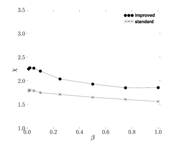
Figure 8: Minimum FN Selection comparison

Figure 9: Maximum FP Selection comparison

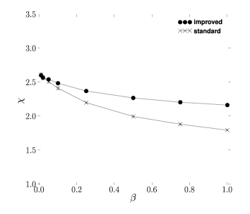
Figure 10: Ratio Selection comparison

Fig. 10 to Fig. 10 compare the performances of our improved selective clearing algorithms to the standard selective clearing algorithms. The horizontal axis shows $\beta$, the ratio of the quantity of troublesome keys to remove to the whole false positive set (see eqn. 17). The vertical axis gives $\chi$, the ratio between the proportion of false positives removed and the proportion of false negatives generated (see eqn. 12).

We see that our improved selective clearing algorithms perform better than those described in Sec. IV. In particular, Improved Minimum FN Selection provides the strongest increase compared to the standard algorithm: between 66.048% ($\beta=0.01$) and 84.129% ($\beta=0.75$). Improved Maximum FN Selection and Improved Ratio Selection provides better results, compared to the standard version of the algorithms, when $\beta$ is high. Finally, Improved Ratio Selection provides the best results, as expected from standard selective clearing algorithms.

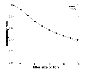
(a) Filled proportion of the ElementList vector

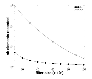
(b) Average ElementList size

Figure 11: ElementList vector evaluation

Fig. 11 evaluates the ElementList vector data structure. The horizontal axis, for both plots, gives the vector size, $m$. We vary it between 10⁴ and 10⁵, with an increment of 10⁴.

Fig. 11(a) shows, on the vertical axis, the proportion of the vector that is used. If it is equal to 1, it means that all cells in the vector contain, at least, one element. Otherwise, if it is equal to 0, it means that all the vector cells are empty. We see from Fig. 11(a) that the occupancy rate of the vector decreases nearly linearly with the vector size. We also notice that the occupancy rate of both vector, $v_{A}$ and $v_{B}$, is the same for most of the vector sizes. When the vector is larger, i.e., above 90,000 cells, the occupancy rate of $v_{B}$ becomes smaller than $v_{A}$.

Fig. 11(b) shows, on the vertical axis, the average size of an ElementList item in the vector. The minimum size is 1 (otherwise, the list is empty). The maximum value is either $|A|$, for $v_{A}$, either $|B|$, for $v_{B}$. For our experiments, we consider that $B$ equals $FP$. Looking first at the $v_{B}$ vector, one can see that the average ElementList size decreases quickly when the vector size increase. It decreases by two order of magnitude while the vector size increases only by one order. Looking now at the $v_{A}$ vector, we see that in the worst case, a cell contains, on average, less than ten elements. It quickly decreases until having, at worst, one element per filled cell.

VI Case Study

VI-A Tracing Paths with a Red Stop Set

Retouched Bloom filters can be applied across a wide range of applications that would otherwise use Bloom filters. For RBFs to be suitable for an application, two criteria must be satisfied. First, the application must be capable of identifying instances of false positives. Second, the application must accept the generation of false negatives, and in particular, the marginal benefit of removing the false positives must exceed the marginal cost of introducing the false negatives.

This section describes the application that motivated our introduction of RBFs: a network measurement system that traces routes, and must communicate information concerning IP addresses at which to stop tracing. Sec. VII-B will investigate others applications that can benefit from RBFs instead of Bloom filters. Sec. VI-B evaluates the impact of using RBFs in this application.

Maps of the internet at the IP level are constructed by tracing routes from measurement points distributed throughout the internet. The skitter system [8], which has provided data for many network topology papers, launches probes from 24 monitors towards almost a million destinations. However, a more accurate picture can potentially be built by using a larger number of vantage points. Dimes [9] heralds a new generation of large-scale systems, counting, at present 8,700 agents distributed over five continents. As Donnet et al. [10] (including authors on the present paper) have pointed out, one of the dangers posed by a large number of monitors probing towards a common set of destinations is that the traffic may easily be mistaken for a distributed denial of service (DDoS) attack.

One way to avoid such a risk would be to avoid hitting destinations. This can be done through smart route tracing algorithms, such as Donnet et al.’s Doubletree. With Doubletree, monitors communicate amongst themselves regarding routes that they have already traced, in order to avoid duplicating work. Since one monitor will stop tracing a route when it reaches a point that another monitor has already traced, it will not continue through to hit the destination.

Doubletree considerably reduces, but does not entirely eliminate, DDoS risk. Some monitors will continue to hit destinations, and will do so repeatedly. One way to further scale back the impact on destinations would be to introduce an additional stopping rule that requires any monitor to stop tracing when it reaches a node that is one hop before that destination. We call such a node the penultimate node, and we call the set of penultimate nodes the red stop set (RSS).Fig. 12 illustrates the RSS concept, showing penultimate nodes as grey discs.

A monitor is typically not blocked by its own first-hop node, as it will normally see a different IP address from the addresses that appear as penultimate nodes on incoming traces. This is because a router has multiple interfaces, and the IP address that is revealed is supposed to be the one that sends the probe reply. The application that we study in this paper conducts standard route traces with an RSS. We do not use Doubletree, so as to avoid having to disentangle the effects of using two different stopping rules at the same time.

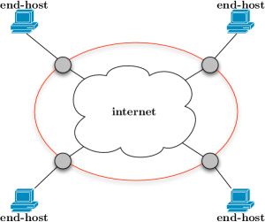
Figure 12: Red stop set

How does one build the red stop set? The penultimate nodes cannot be determined a priori. However, the RSS can be constructed during a learning round in which each monitor performs a full set of standard traceroutes, i.e., until hitting a destination. Monitors then share their RSSes. For simplicity, we consider that they all send their RSSes to a central server, which combines them to form a global RSS, that is then redispatched to the monitors. The monitors then apply the global RSS in a stopping rule over multiple rounds of probing.

Destinations are only hit during the learning round and as a result of errors in the probing rounds. DDoS risk diminishes with an increase in the ratio of probing rounds to learning rounds, and with a decrease in errors during the probing rounds. DDoS risk would be further reduced were we to apply Doubletree in the learning round, as the number of probes that reach destinations during the learning round would then scale less then linearly in the number of monitors. However, our focus here is on the probing rounds, which use the global RSS, and not on improving the efficiency of the learning round, which generates the RSS, and for which we already have known techniques.

The communication cost for sharing the RSS among monitors is linear in the number of monitors and in the size of the RSS representation. It is this latter size that we would like to reduce by a constant compression factor. If the RSS is implemented as a list of 32-bit vectors, skitter’s million destinations would consume 4 MB. We therefore propose encoding the RSS information in Bloom filters. Note that the central server can combine similarly constructed Bloom filters from multiple monitors, through bitwise logical or operations, to form the filter that encodes the global RSS.

The cost of using Bloom filters is that the application will encounter false positives. A false positive, in our case study, corresponds to an early stop in the probing, i.e., before the penultimate node. We call such an error stopping short, and it means that part of the path that should have been discovered will go unexplored. Stopping short can also arise through network dynamics, when additional nodes are introduced, by routing changes or IP address reassignment, between the previously penultimate node and the destination. In contrast, a trace that stops at a penultimate node is deemed a success. A trace that hits a destination is called a collision. Collisions might occur because of a false negative for the penultimate node, or simply because routing dynamics have introduced a new path to the destination, and the penultimate node on that path was previously unknown.

As we show in Sec. VI-B, the cost of stopping short is far from negligible. If a node that has a high betweenness centrality (Dall’Asta et al. [11] point out the importance of this parameter for topology exploration) generates a false positive, then the topology information loss might be high. Consequently, our idea is to encode the RSS in an RBF.

There are two criteria for being able to profitably employ RBFs, and they are both met by this application. First, false positives can be identified and removed. Once the topology has been revealed, each node can be tested against the Bloom filter, and those that register positive but are not penultimate nodes are false positives. The application has the possibility of removing the most troublesome false positives by using one of the selective algorithms discussed in Sec. IV. Second, a low rate of false negatives is acceptable and the marginal benefit of removing the most troublesome false positives exceeds the marginal cost of introducing those false negatives. Our aim is not to eliminate collisions; if they are considerably reduced, the DDoS risk has been diminished and the RSS application can be deemed a success. On the other hand, systematically stopping short at central nodes can severely restrict topology exploration, and so we are willing to accept a low rate of random collisions in order to trace more effectively. These trade-offs are explored in the Sec. VI-B.

Implementation	Positive				Negative
	Success	Topo. discovery	Compression	No Collision	Topo. missed	Load	Collision
List	X	X		X		X
Bloom filter			X	X	X
RBF	X	X	X				X

TABLE V: Positive and negative aspects of each RSS implementation

Table V summarizes the positive and negative aspects of each RSS implementation we propose. Positive aspects are a success, stopping at the majority of penultimate nodes, topology information discovered, the eventual compression ratio of the implementation and a minimum number of collisions with destinations. Negative aspects of an implementation can be the topology information missed due to stopping short, the load on the network when exchanging the RSS and the risk of hitting destinations too much times. Sec. VI-B will measure the positive and negative aspects of each implementation.

VI-B Evaluation

In this section, we evaluate the use of RBFs in a tracerouting system based on an RSS. We first present our methodology and then, discuss our results.

VI-B1 Methodology

Our study was based on skitter data [8] from January 2006. This data set was generated by 24 monitors located in the United States of America, Canada, the United Kingdom, France, Sweden, the Netherlands, Japan, and New Zealand. The monitors share a common destination set of 971,080 IPv4 addresses. Each monitor cycles through the destination set at its own rate, taking typically three days to complete a cycle.

For the purpose of our study, in order to reduce computing time to a manageable level, we worked from a limited set of 10 skitter monitors, all the monitors sharing a list of 10,000 destinations, randomly chosen from the original set. In our data set, the RSS contains 8,006 different IPv4 addresses.

We will compare the three RSS implementations discussed above: list, Bloom filter and RBF. The list would not return any errors if the network were static, however, as discussed above, network dynamics lead to a certain error rate of both collisions and instances of stopping short.

For the RBF implementation, we considered $\beta$ values (see eqn. 17) of 1%, 5%, 10% and 25%. We further applied the Ratio Selection algorithm, as defined in Sec. IV-A. For the Bloom filter and RBF implementations, the hashing was emulated with random numbers. We simulate randomness with the Mersenne Twister MT19937 pseudo-random number generator [6].

To obtain our results, we simulated one learning round on a first cycle of traceroutes from each monitor, to generate the RSS. We then simulated one probing round, using a second cycle of traceroutes. In this simulation, we replayed the traceroutes, but applied the stopping rule based on the RSS, noting instances of stopping short, successes, and collisions.

VI-B2 Results

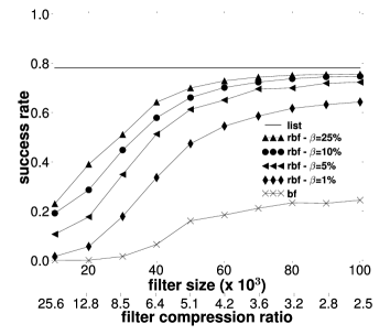
Figure 13: Success rate

Fig. 13 compares the success rate, i.e., stopping at a penultimate node, of the three RSS implementations. The horizontal axis gives different filters size, from 10,000 to 100,000, with an increment of 10,000. Below the horizontal axis sits another axis that indicates the compression ratio of the filter, compared to the list implementation of the RSS. The vertical axis gives the success rate. A value of 0 would mean that using a particular implementation precludes stopping at the penultimate node. On the other hand, a value of 1 means that the implementation succeeds in stopping each time at the penultimate node.

Looking first at the list implementation (the horizontal line), we see that the list implementation success rate is not 1 but, rather, 0.7812. As explained in Sec. VI-B, this can be explained by the network dynamics such as routing changes and dynamic IP address allocation.

With regards to the Bloom filter implementation, we see that the results are poor. The maximum success rate, 0.2446, is obtained when the filter size is 100,000 (a compression ratio of 2.5 compared to the list). Such poor results can be explained by the troublesomeness of false positives. Fig. 14 shows, in log-log scale, the troublesomeness distribution of false positives. The horizontal axis gives the troublesomeness degree, defined as the number of traceroutes that stop short for a given key. The maximum value is $10^{4}$, i.e., the number of traceroutes performed by a monitor. The vertical axis gives the number of false positive elements having a specific troublesomeness degree. The most troublesome keys are indicated by an arrow towards the lower right of the graph: nine false positives are, each one, encountered 10,000 times.

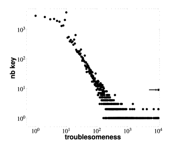
Figure 14: Troublesomeness distribution

Looking now, in Fig. 13, at the success rate of the RBF, we see that the maximum success rate is reached when $\beta$ = 0.25. We also note a significant increase in the success rate for RBF sizes from 10,000 to 60,000. After that point, except for $\beta$ = 1%, the increase is less marked and the success rate converges to the maximum, 0.7564. When $\beta$ = 0.25, for compression ratios of 4.2 and lower, the success rate approaches that of the list implementation. Even for compression ratios as high as 25.6, it is possible to have a success rate over a quarter of that offered by the list implementation.

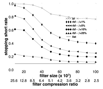
Figure 15: Stopping short rate

Fig. 15 gives the stopping short rate of the three RSS implementations. A value of 0 means that the RSS implementation does not generate any instances of stopping short. On the other hand, a value of 1 means that every stop was short.

Looking first at the list implementation, one can see that the stopping short rate is 0.0936. Again, network dynamics imply that some nodes that were considered as penultimate nodes during the learning phase are no longer located one hop before a destination.

Regarding the Bloom filter implementation, one can see that the stopping short rate is significant. Between 0.9981 (filter size of 10³) and 0.7668 (filter size of 10⁴). The cost of these high levels of stopping short can be evaluated in terms of topology information missed. Fig. 16 compares the RBF and the Bloom filter implementation in terms of nodes (Fig. 16(a)) and links (Fig. 16(b)) missed due to stopping short. A value of 1 means that the filter implementation missed all nodes and links when compared to the list implementation. On the other hand, a value of 0 mean that there is no loss, and all nodes and links discovered by the list implementation are discovered by the filter implementation. One can see that the loss, when using a Bloom filter, is above 80% for filter sizes below 70,000.

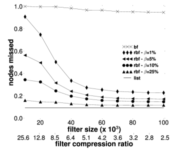
(a) nodes

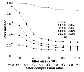
(b) links

Figure 16: Topology information missed

Implementing the RSS as an RBF allows one to decrease the stopping short rate. When removing 25% of the most troublesome false positives, one is able to reduce the stopping short between 76.17% (filter size of 10³) and 84,35% (filter size of 10⁴). Fig. 15 shows the advantage of using an RBF instead of a Bloom filter. Fig. 16 shows this advantage in terms of topology information. We miss a much smaller quantity of nodes and links with RBFs than Bloom filters and we are able to nearly reach the same level of coverage as with the list implementation.

Fig. 17 shows the cost in terms of collisions. Collisions will arise under Bloom filter and list implementations only due to network dynamics. Collisions can be reduced under all RSS implementations due to a high rate of stopping short (though this is, of course, not desired). The effect of stopping short is most pronounced for RBFs when $\beta$ is low, as shown by the curve $\beta=0.01$. One startling revelation of this figure is that even for fairly high values of $\beta$, such as $\beta=0.10$, the effect of stopping short keeps the RBF collision cost lower than the collision cost for the list implementation, over a wide range of compression ratios. Even at $\beta=0.25$, the RBF collision cost is only slightly higher.

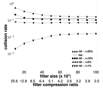
Figure 17: Collision cost

Fig. 18 compares the success, stopping short, and collision rates for the RBF implementation with a fixed filter size of 60,000 bits. We vary $\beta$ from 0.01 to 1 with an increment of 0.01. We see that the success rate increases with $\beta$ until reaching a peak at 0.642 ($\beta$ = 0.24), after which it decreases until the minimum success rate, 0.4575, is reached at $\beta$ = 1. As expected, the stopping short rate decreases with $\beta$, varying from 0.6842 ($\beta$ = 0) to 0 ($\beta$ = 1). On the other hand, the collision rate increases with $\beta$, varying from 0.0081 ($\beta$ = 0) to 0.5387 ($\beta$ = 1).

The shaded area in Fig. 18 delimits a range of $\beta$ values for which success rates are highest, and collision rates are relatively low. This implementation gives a compression ratio of 4.2 compared to the list implementation. The range of $\beta$ values (between 0.1 and 0.3) gives a success rate between 0.7015 and 0.7218 while the list provides a success rate of 0.7812. The collision rate is between 0.1073 and 0.1987, meaning that in less than 20% of the cases a probe will hit a destination. On the other hand, a probe hits a destination in 12.51% of the cases with the list implementation. Finally, the stopping short rate is between 0.2355 and 0.1168 while the list implementation gives a stopping short rate of 0.0936.

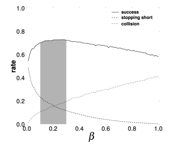
Figure 18: Metrics for an RBF with m=60,000

Fig. 19 illustrates the behavior of the RSS during ten traceroute cycle. We consider the list and the RBF implementations. The RBF is tuned as followed: the vector is 60,000 bits long and $\beta$ is 0.25. These values are suggested by previous studies in this section. The horizontal axis, in Fig. 19, gives the ten cycles, the cycle labeled $C_{1}$ is equivalent to the results discussed below. The vertical axis gives the metric rate (i.e., success, stopping short and collision).

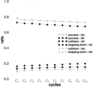
Figure 19: Metrics for 10 traceroute cycles

In Fig. 19, one can see the degradation of the RSS performances. The success rate decreases with time while the stopping short and the collision rates increases with time. However, both implementation behaves in the same way. The decrease of the success rate for the RBF is somewhat similar to the list one. The same conclusion holds for the stopping short and collision rates. Fig. 19 shows thus the robustness of the RBF.

In closing, we emphasize that the construction of $B$ and the choice of $\beta$ in this case study are application specific. We do not provide guidelines for a universal means of determining which false positives should be considered particularly troublesome, and thus subject to removal, across all applications. However, it should be possible for other applications to measure, in a similar manner as was done here, the potential benefits of introducing RBFs.

VI-C Comparing Selective Clearing Algorithms

In this section, we compare the performances of the Ratio Selection algorithm and the Improved Ratio Selection algorithm for our case study. The methodology applied was the same than the one described in Sec. VI-B1, except that we did not consider the Bloom filter implementation of the RSS. In order to make the plots readable, we only took into account $\beta=0.01$ and $\beta=0.25$.

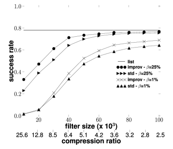
Figure 20: Success comparison

Fig. 20 compares both selective clearing techniques regarding the success metric. Recall that a success occurs when a trace stops at a penultimate node. The horizontal axis gives different filters size, from 10,000 to 100,000, with an increment of 10,000. Below the horizontal axis sits another axis that indicates the compression ratio of the filter, compared to the list implementation of the RSS. The vertical axis gives the success rate. A value of 0 would mean that using a particular implementation precludes stopping at the penultimate node. On the other hand, a value of 1 means that the implementation succeeds in stopping each time at the penultimate node.

We see, from Fig. 20, that Improved Ratio Selection performs better than standard Ratio Selection. For $\beta=0.01$, the increase is more important for larger vector size while it is the contrary for $\beta=0.25$.

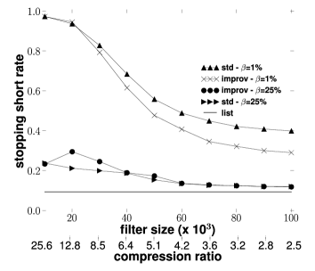
Figure 21: Stopping short comparison

Fig. 21 compares both selective clearing techniques regarding the stopping short metric. Recall that a stopping short corresponds to an early stop in the probing, i.e., before the penultimate node.

Again, we see from Fig. 21 that the improved selective clearing algorithms performs better than standard algorithms. This is more explicit when $\beta=0.01$ and the vector is large. However, for $\beta=0.25$, we notice a small increase in the stopping short rate for some vector sizes (between 20,000 and 30,000).

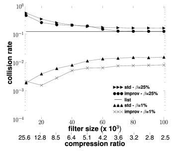
Figure 22: Collision comparison

Fig. 22 compares both selective clearing techniques regarding the collision metric. Recall that a collision occurs when a trace hits a destination.

We note, from Fig. 22, that Improved Ratio Selection can decrease the collision rate compared to standard Ratio Selection. We further see that the collision rate, for Improved Ratio Selection, is very close to the list one when the vector size is higher than 70,000 bits. There is a very tight difference between Improved Ratio Selection and the list that is not visible on Fig. 22.

In this section, we showed that using our improved selective clearing algorithms can improve the performances of the RSS application. Further, this performance increase allows one to more reduce the size of the bit vector, leading to a better compression ratio.

VII Related Work

Early suggestions of applications for Bloom filters were for dictionaries and databases. Bloom’s original paper [1] describes their use for hyphenation. Another dictionary application is for spell-checkers [12, 13]. For databases, they have been suggested to speed up semi-join operations [14, 15] and for differential files [16, 17].

In this section, we discuss related work. Our approach is double: first, we discuss Bloom filters variations and develop those that allow false negatives to arise (Sec. VII-A). Second, we discuss networking applications of Bloom filters and show that RBFs can find a suitable usage for some of them (Sec. VII-B)

VII-A Bloom Filters Variations

VII-A1 Extensions

Time-Decaying Bloom filters (TBF), proposed by Cheng et al. [18], are somewhat similar to counting Bloom filters [5] (CBF) as the standard bit vector is replaced by an array of counters. TBF differs from CBF as values in the array decay periodically with time elapsing. TBF are used for maintaining time sensitive profiles of the web. As only a small proportion of web content are frequently visited, Cheng et al. propose that only heavy hitters are monitored by large counters, in order to avoid allocation larger counters to small values.

Chang et al.’s extension aims at supporting multiple binary predicates as opposed to single binary predicate (the key $x$ belongs or not to $A$) of a traditional Bloom filter [19]. Such an extension is needed in packet classification, for instance, where a packet can be classified into many, possibly disjoint, sets. If the considered application required $I$ different sets, each cell of the bit vector will contained $I$ bits where the $i^{th}$ bit in a cell corresponds to the $i^{th}$ set. When the filter is queried for a key membership, the $k$ bit strings returned by the hash functions are AND. In the resulting bit string, if the $i^{th}$ bit is set to 1, it means that the key might belong to $i^{th}$ set. The case where more than one bit is set to 1 after the AND is not addressed by Chang et al.

The time-out Bloom filters [20], developed by Kong et al. in the context of packet sampling, is an extension to standard Bloom filters where the bit vector is replaced by a bucket vector, each bucket containing a timestamp. A bucket time-out $t_{0}$ is associated to the time-out Bloom filter. A time-out Bloom filter allows one to determine if an incoming packet belongs to an active flow or it is the first packet of a new flow. When a packet with a timestamp $t$ arrives, it is compared with the $k$ timestamps, $v[h_{1}(t)],v[h_{2}(t)],\ldots,v[h_{k}(t)]$. If at least one of the $k$ timestamps recorded in the filter follows $t-v[h_{i}(t)]>t_{0}$ (i.e., the bucket is time-out), the packet is sampled. Otherwise, it is discarded. After the comparison, all the $k$ positions in the vector are updated with $t$ even if the packet is not sampled and all other buckets in the vector are set to 0. In a time-out Bloom filter, a bucket getting time-out is equivalent to a standard Bloom filter having a bit to 0, while a non time-out is the same as a bit to 1 in a Bloom filter. Due to false positives, an time-out Bloom filter does not guarantee that all first packets can be sampled.

Kirsch and Mitzenmacher show that only two hash functions are needed to effectively implement a Bloom filter without any loss in the false positive probability [21]. It also leads to less computation. The idea is to use two hash functions $h_{1}(x)$ and $h_{2}(x)$ for simulation additional hash functions of the form $g_{i}(x)~{}=~{}h_{1}(x)~{}+~{}ih_{2}(x)$.

Space-code Bloom filters by Kumar et al. [22] and spectral Bloom filters by Cohen and Matias [23] are approximate representation of a multiset, which allows for querying “How many occurrences of $x$ are there in set $M$?”. A multiset is a set in which each member has a multiplicity, i.e., a natural number indicating the occurrence of a member in the set.

Based on the observation that, in many applications, some popular elements are queried much frequently than the others, Bruck et al. propose the weighted Bloom filters (WBF) [24]. If the query frequency or the membership likelihood is not uniform over all the keys in the universe, the traditional configuration of the Bloom filter does not give the optimal performance, as we demonstrated in Sec. VI-B. In a WBF, each key $e\in U$ is assigned $k_{e}$ hash functions, where $k_{e}$ depends on the query frequency of $e$ and its likelihood of being a member of $A$. Each non-member element has a different false positive probability. The average false positive probability of a WBF is given by the weighted sum over the queries frequencies of the elements in the universe. A key is assigned more hash functions if its query frequency is high and its chance of being a member is low. When the query frequencies and the membership likelihoods are the same for all keys in $U$, a WBF behaves like a traditional Bloom filter.

The WBF differs from our RBF as it tries to build the Bloom filter in such a way that it reflects the key distribution. However, it is not clear how a WBF can be used has a message shared between distributed entities as each key is, potentially, assigned a different number of hash functions. There is an additional storage information associated to a WBF while an RBF modifies the traditional Bloom filter without adding any information.

Standard Bloom filters and most of their extensions are approaches to represent a static set, i.e., the size of $A$ does not evolve with time. However, for many applications, for instance large-scale and distributed systems, it is difficult to foresee the threshold size for the set $A$. It is possible that the size of $A$ will exceed its initial size, $n_{0}$, during the execution of the application. It is thus difficult, even impossible, to maintain the false positive rate and the false positive probability will exceed its threshold. Consequently, the Bloom filter can become unusable under such a scenario.

Two extensions of the standard Bloom filters have been proposed in order to support dynamic sets. The first one, split Bloom filters [25], uses a constant $s\times m$ bit matrix to represent a set, where $s$ is a constant and must be pre-defined according to the estimation of the maximum value of set size. The second one, dynamic Bloom filters [26] (DBF) proposed by Guo et al., also makes use of a $s\times m$ bit matrix but each of the $s$ rows is a standard Bloom filter. The creation process of a DBF is iterative. At the starting, the DBF is a $1\times m$ bit matrix, i.e., it is composed of a single standard Bloom filter. It supposed that $n_{r}$ elements are recorded in the initial bit vector, where $n_{r}\leq n$. As the size of $A$ grows during the execution of the application, several keys must be inserted in the DBF. When inserting a key into the DBF, one must first get an active Bloom filter in the matrix. A Bloom filter is active when the number of recorded keys, $n_{r}$, is strictly less than the current cardinality of $A$, $n$. If an active Bloom filter is found, the key is inserted and $n_{r}$ is incremented by one. On the other hand, if there is no active Bloom filter, a new one is created (i.e., a new row is added to the matrix) according to the current size of $A$ and the element is added in this new Bloom filter and the $n_{r}$ value of this new Bloom filter is set to one. A given key is said to belong to the DBF if the $k$ positions are set to one in one of the matrix rows. Guo et al. also extend standard Bloom filters and DBF for supporting set consisted of multi-attribute keys.

VII-A2 Bloom Filters and False Negatives

Has nobody thought of the RBF before? There is a considerable literature on Bloom filters, and their applications in networking, that we discuss in Sec. VII-B. In a few instances, suggested variants on Bloom filters do allow false negatives to arise. However, these variants do not preserve the size of the standard Bloom filter, as RBFs do. Nor have the false negatives been the subject of any analytic or simulation studies. In particular, the possibility of explicitly trading off false positives for false negatives has not been studied prior to the current work, and efficient means for performing such a trade-off have not been proposed.

First is the anti-Bloom filter, which was suggested in non-peer reviewed work [27, 28]. An anti-Bloom filter is composed of a standard Bloom filter plus a separate smaller filter that can be used to override selected positive results from the main filter. When queried, a negative result is generated if either the main filter does not recognize a key or the anti-filter does. The anti-Bloom filter requires more space than the standard filter, but the space efficiency has not been studied. Nor have studies been made of the impact of the anti-filter on the false positive rate, or on the false negatives that would be generated.

Second, Fan et al.’s CBF replaces each cell of a Bloom filter’s bit vector with a four-bit counter, so that instead of storing a simple 0 or a 1, the cell stores a value between 0 and 15 [5]. This additional space allows CBFs to not only encode set membership information, as standard Bloom filters do, but to also permit dynamic additions and deletions to that information. One consequence of this new flexibility is that there is a chance of generating false negatives. They can arise if counters overflow. Fan et al. suggest that the counters be sized to keep the probability of false negatives to such a low threshold that they are not a factor for the application (four bits being adequate in their case). The possibility of trading off false positives for false negatives is not entertained.

Third, Bonani et al.’s $d$-left CBF is an improvement on the CBF. As with the CBF, it can produce false negatives. It can also produce another type of error called “don’t know”. Bonani et al. conduct experiments in which they measure the rates for the different kinds of errors, but here too there is no examination of the possibility of trading off false positives against false negatives. The $d$-left CBF is more space-efficient than the CBF. But CBFs themselves require a constant multiple more space than standard Bloom filters, and the question does not arise of comparing the space efficiency of $d$-left CBFs with that of standard Bloom filters, as they serve different functions.

Four, Song et al. [7] propose an extension to the CBF, called the extended Bloom filter (EBF), in order to support exact address prefix matching for routing. An array is associated to the CBF. Each cell of this array contains the list of keys that are recorded in the corresponding cell in the CBF. Song et al. propose several techniques to reduce the memory cost of the EBFs. The EBFs are designed to achieved higher lookup performance within high-speed routers.

With the EBFs, the false positives are removed by adding information to the CBFs. With the RBFs, by contrast, no information is added to remove the false positives. The cost of these removals is expressed in terms of false negatives generated for the RBFs and in terms of increased memory usage for the EBFs.

Five, Laufer et al. [29] an extension to the standard Bloom filter called the generalized Bloom filter (GBF). With the GBF, one moves beyond the notion that elements must be encoded with 1s, and that 0s represent the absence of information. A GBF starts out as an arbitrary vector of both 1s and 0s, and information is encoded by setting chosen bits to either 0 or 1. As a result, the GBF is a more general binary classifier than the standard Bloom filter. One consequence is that it can produce either false positives or false negatives. Laufer et al. provide a careful analysis [30] of the trade-offs between false positives and false negatives.

A GBF employs two sets of hash functions, $g_{1},\ldots,g_{k_{0}}$ and $h_{1},\ldots,h_{k_{1}}$ to set and reset bits. To add an element $x$ to the GBF, the bits at positions $g_{1}(x),\ldots,g_{k_{0}}(x)$ are set to 0 and the bits at positions $h_{1}(x),\ldots,h_{k_{1}}(x)$ are set to 1. In the case of a collision between two hash values $g_{i}(x)$ and $h_{j}(x)$, the bit is set to 0. The membership of an element $y$ is verified by checking if all bits at $g_{1}(y),\ldots,g_{k_{0}}(y)$ are set to 0 and all bits at $h_{1}(y),\ldots,h_{k_{1}}(y)$ are set to 1. If at least one bit is inverted, $y$ does not belong to the GBF with a high probability. A false negative arises when at least one bit of $g_{1}(y),\ldots,g_{k_{0}}(y)$ is set to 1 or one bit of $h_{1}(y),\ldots,h_{k_{1}}(y)$ is set to 0 by another element inserted afterwards. The rates of false positives and false negatives in a GBF can be traded off by varying the numbers of hash functions, $k_{0}$ and $k_{1}$, as well as other parameters such as the size of the filter.

RBFs differ from GBFs in that they allow the explicit removal of selected false positives. RBFs also do so in a way that allows the overall error rate, expressed as a combination of false positives and false negatives, to be lowered as compared to a standard Bloom filter of the same size. We note that the techniques used to remove false positives from standard Bloom filters could be extended to remove false positives from GBFs. For a false positive key, $x$, either one would set one of the bits $g_{1}(x),\ldots,g_{k_{0}}(x)$ to 1 or one of the bits $h_{1}(x),\ldots,h_{k_{1}}(x)$ to 0.

Finally, Distance-sensitive Bloom filters, introduced by Kirsch and Mitzenmacher [31], consider the notion of an “approximate Bloom filter”, that allows approximate instead of exact matches under a distance metric. In other words, a distance-sensitive Bloom filter tries to answer the following question: “Is $x$, where $x\in U$, close to an element belonging to $A$?”. In a distance-sensitive Bloom filter, classic hash functions are replaced by distance-sensitive hash functions. A Distance-sensitive Bloom filter allow false positives and false negatives.

One might think that there would be general binary classifiers similar to RBFs in the domain of machine learning. It is usual in artificial intelligence to make use of classifiers, such as neural networks, Bayesian classifiers (naive or not), or support vector machines (SVMs) [32, 33]. However, these classifiers differ from RBFs in that they classify based on feature or attribute vectors. RBFs classify elements purely on the basis of their unique keys.

VII-B Networking Bloom Filters Applications

Bloom filters have been widely used in networking applications, as stated by Broder and Mitzenmacher [3]. Broder and Mitzenmacher consider four types of networking applications: overlays and peer-to-peer networks, resource processing, packet routing and measurement. All these fours categories are developed below. For each of them, we discuss the use of RBFs instead of traditional Bloom filters.

VII-B1 Overlays and Peer-to-Peer

For a node in a peer-to-peer file sharing system, keeping a list of objects stored at all other nodes might be costly in terms of memory, but keeping Bloom filters for all other nodes might be an attractive alternative. This was proposed by Cuenca-Acuna et al. for their PlanetP system [34].

PlanetP meets the two criteria for the use of RBFs. First, the application can identify false positives. A node, through is own experience with the inability to locate certain files at the expected nodes, can determine that the keys corresponding to those files yield false positives. Second, false negatives are tolerated because not every node that stores a given object need be identified. In a file sharing system, the same object is typically stored in multiple locations, and so the failure of one node to recognize some of the locations for some of the objects should not pose a great problem, provided the rate of such errors remains within reasonable bounds. The communications savings that come from eliminating some false positives might well outweigh the costs of missing some locations.

Byers et al. [35] propose an application for distributing large files to many peers in overlay networks. They suggest that peers may want to solve approximate set reconciliation problems. The idea is to allow a peer A to send to a peer B objects that B does not have. Encoding the sets of objects as Bloom filters allows for data compression. B will send A its Bloom filter. Testing its own set, element by element, against this Bloom filter allows A to know the set of objects B does not have, and send them to B. Because of false positives, not all objects that B needs will be sent, but most will.

Approximate set reconciliation clearly meets the second criterion for using RBFs. A low rate of false negatives in the RBF furnished by peer B would result in peer A sending a small number of elements that B already possesses. It is easy to imagine that the system designers would be willing to pay this communications overhead price in order to ensure that B gets more of the elements that it is missing.

A question arises, however, for the first criterion. How does peer B identify the false positives in the Bloom filter that it sends out? For this, it would need to know the keys for the objects that it is missing. For some applications, this would not be possible. But we could easily imagine many applications where the keys are known. For instance, B might know the contents of a music catalog, but not have many of the songs in that catalog. It could identify the false positives in its RBF by testing the keys in the catalog one by one.

Rhea et al. [36] describe a probabilistic algorithm for routing peer-to-peer resource location queries. Each node in the network keeps an array of Bloom filters, called an attenuated Bloom filter, for each adjacent edge in the overlay topology. In the array for each edge, there is a Bloom filter for each distance $d$, up to a maximum value, so that the $d^{th}$ Bloom filter in the array keeps track of resources available via $d$ hops through the overlay network along that edge. If it is deemed probable that the resource that is being searched for is present, the query is routed to the nearest neighbor. This scheme would require the addition of feedback to identify false positives. If false positives could be identified, they could be removed. This might be worthwhile, as false negatives do not invalidate the system. The array of Bloom filters could be replaced by an array of RBFs, bringing about a decrease in the false positive rate at the cost of a comparatively small increase in the false negative rate.

VII-B2 Resource Routing

Czerwinski et al. [37] describe a resource discovery architecture called Ninja, that makes use of Bloom filters. In our judgment, Ninja would not be tolerant of false negatives, and is thus not a candidate for using RBFs.

However, another resource routing application could benefit. Rhea et al. [36] describe a probabilistic algorithm for routing peer-to-peer resource location queries. Each node in the network keeps an array of Bloom filters, called an attenuated Bloom filter, for each adjacent edge in the overlay topology. In the array for each edge, there is a Bloom filter for each distance $d$, up to a maximum value, so that the $d^{th}$ Bloom filter in the array keeps track of resources available via $d$ hops through the overlay network along that edge. If it is deemed probable that the resource that is being searched for is present, the query is routed to the nearest neighbor. This scheme would require the addition of feedback to identify false positives. If false positives could be identified, they could be removed. This might be worthwhile, as false negatives do not invalidate the system. The array of Bloom filters could be replaced by an array of RBFs, bringing about a decrease in the false positive rate at the cost of a comparatively small increase in the false negative rate.

VII-B3 Network Packet Processing

Dharmapurikar et al. [38] propose the use of Bloom filters for detecting predefined signatures in packet payloads. They propose an architecture of $W$ parallel Bloom filters, each Bloom filter focusing on strings of a specified length. If a string is found to be a member of any Bloom filter, it is then declared as a possible matching signature. To avoid the risk of false positives, each matching signature is tested in an analyzer which determines if the signature is truly a member of the set $A$ or not. In other words, the analyzer contains all elements of $A$. Bloom filters are only used to discard elements not belonging to $A$.

At least one of the two criteria for using the RBFs is met in the process described by Dharmapurikar et al. The analyzer offers the opportunity to identify false positives. The application should obtain a gain in terms of processing time by removing from the filters those false positives. The second criterion is application-specific. If a small rate of false negatives may be tolerated, then RBFs are suitable.

VII-B4 Measurement

Bloom filters are also used in topology discovery. Some authors of this paper propose Doubletree [10], an efficient and cooperative algorithm that aims to reduce redundancy, i.e., duplication of effort, in tracerouting systems by taking into account the tree-like structure of routes in the internet. Reducing the redundancy implies coordination between Doubletree monitors by sharing information about what was previously discovered. To summarize this information shared, Donnet et al. propose to implement it using Bloom filters [39]. Though it is difficult for Doubletree monitors to meet the first criterion by detecting false positives, we proposed, in this paper (see Sec. VI), a variant of the problem for which RBFs are well adapted.

VIII Conclusion

References

- [1] B. H. Bloom, “Space/time trade-offs in hash coding with allowable errors,” Communications of the ACM, vol. 13, no. 7, pp. 422–426, 1970.
- [2] M. Mitzenmacher, “Compressed Bloom filters,” IEEE/ACM Transactions on Networking, vol. 10, no. 5, pp. 604–612, 2002.
- [3] A. Broder and M. Mitzenmacher, “Network applications of Bloom filters: A survey,” Internet Mathematics, vol. 1, no. 4, pp. 485–509, 2002.
- [4] F. Bonomi, M. Mitzenmacher, R. Panigraphy, S. Singh, and G. Varghese, “Beyond Bloom filters: From approximate membership checks to approximate state machines,” in Proc. ACM SIGCOMM, Sept. 2006, pp. 315–326.
- [5] L. Fan, P. Cao, J. Almeida, and A. Z. Broder, “Summary cache: a scalable wide-area Web cache sharing protocol,” IEEE/ACM Transactions on Networking, vol. 8, no. 3, pp. 281–293, 2000.
- [6] M. Matsumoto and T. Nishimura, “Mersenne Twister: A 623-dimensionally equidistributed uniform pseudorandom number generator,” ACM Trans. on Modeling and Computer Simulation, vol. 8, no. 1, pp. 3–30, Jan. 1998.
- [7] H. Song, S. Dharmapurikar, J. Turner, and J. Lockwood, “Fast hash table lookup using extended Bloom filter: An aid to network processing,” in Proc. ACM SIGCOMM, Aug. 2005, pp. 181–192.
- [8] B. Huffaker, D. Plummer, D. Moore, and k. claffy, “Topology discovery by active probing,” in Proc. Symposium on Applications and the Internet (SAINT), Jan. 2002, pp. 90–96.
- [9] Y. Shavitt and E. Shir, “DIMES: Let the internet measure itself,” ACM SIGCOMM Computer Communication Review, vol. 35, no. 5, pp. 71–74, 2005.
- [10] B. Donnet, P. Raoult, T. Friedman, and M. Crovella, “Efficient algorithms for large-scale topology discovery,” in Proc. ACM SIGMETRICS, Jun. 2005, pp. 327–338.
- [11] L. Dall’Asta, I. Alvarez-Hamelin, A. Barrat, A. Vázquez, and A. Vespignani, “A statistical approach to the traceroute-like exploration of networks: theory and simulations,” in Proc. CAAN Workshop, Aug. 2004, pp. 140–153.
- [12] M. D. McIlroy, “Development of a spelling list,” IEEE Trans. on Communications, vol. 30, no. 1, pp. 91–99, 1982.
- [13] J. K. Mullin and D. J. Margoliash, “A tale of three spelling checkers,” Software – Practice and Experience, vol. 20, no. 6, pp. 625–630, 1990.
- [14] K. Bratbergsengen, “Hashing methods and relational algebra operations,” in Proc. 10th International Conference on Very Large Databases, Aug. 1984, pp. 323–333.
- [15] P. Valdurez and G. Gardarin, “Join and semijoin algorithms for a multiprocessor database machine,” ACM Transactions on Database Systems, vol. 9, no. 1, pp. 133–161, 1984.
- [16] L. L. Gremilion, “Designing a Bloom filter for differential file access,” Communications of the ACM, vol. 25, pp. 600–604, 1982.
- [17] J. K. Mullin, “A second look at Bloom filters,” Communications of the ACM, vol. 26, no. 8, pp. 570–571, 1983.
- [18] K. Cheng, M. Iwaihara, L. Xiang, and K. Ushijima, “Efficient web profiling by time-decaying Bloom filters,” DBSJ Letters, vol. 4, no. 1, pp. 137–140, Jun. 2005.
- [19] F. Chang, W.-C. Feng, and K. Li, “Approximate caches for packet classification,” in Proc. IEEE INFOCOM, Mar. 2004, pp. 2196–2207.
- [20] S. Kong, X. Shao, and X. Li, “Time-out Bloom filter: A new sampling method for recording more flows,” in Proc. Internation Conference on Information Networking (ICOIN), Jan. 2006.
- [21] A. Kirsch and M. Mitzenmacher, “Less hashing, same performance: Building a better Bloom filter,” in Proc. 14th Annual European Symposium on Algorithms (ESA), Sept. 2006, pp. 456–467.
- [22] A. Kumar, J. Xu, J. Wang, O. Spatschek, and L. Li, “Space-code Bloom filter for efficient per-flow traffic measurement,” in Proc. ACM Internet Measurement Conference (IMC), Oct. 2003, pp. 167–172.
- [23] S. Cohen and Y. Matias, “Spectral Bloom filters,” in Proc. ACM SIGMOD, Jun. 2003, pp. 241–252.
- [24] J. Bruck, J. Gao, and A. Jiang, “Weighted bloom filter,” in Proc. IEEE Internationl Symposium on Information Theory (ISIT), Jul. 2006.
- [25] M. Xiao, Y. Dai, and X. Li, “Split Bloom filters,” Chinese Journal of Electronic, vol. 32, no. 2, pp. 241–245, 2004.
- [26] D. Guo, J. Wu, H. Chen, and X. Luo, “Theory and network applications of dynamic Bloom filters,” in Proc. IEEE INFOCOM, Apr. 2006.
- [27] T. Lavian, “Bloom filters,” 2004, CS 270–Class Notes. See http://www.cs.berkeley.edu/~kamalika/cs270/notes/lecture30b.pdf.
- [28] N. Hardy, “A little Bloom filter theory (and a bag of filter tricks),” 1999, see http://www.cap-lore.com/code/BloomTheory.html.
- [29] R. P. Laufer, P. B. Velloso, D. de O. Cunha, I. M. Moraes, M. D. D. Bicudo, and O. C. M. B. Duarte, “A new IP traceback system against distributed denial-of-service attacks,” in Proc. 12th International Conference on Telecommunications (ICT), May 2005.
- [30] R. P. Laufer, P. B. Velloso, and O. C. M. B. Duarte, “Generalized Bloom filters,” Electrical Engineering Program, COPPE/UFRJ, Tech. Rep., 2005.
- [31] A. Kirsch and M. Mitzenmacher, “Distance-sensitive Bloom filters,” in Proc. Algorithm Engineering and Experiments (ALENEX), Jan. 2006.
- [32] T. Mitchell, Machine Learning. McGraw Hill, 1997.
- [33] S. J. Russell and P. Norvig, Artificial Intelligence: A Modern Approach, 2nd ed. Prentice Hall, 2003.
- [34] F. M. Cuenca-Acuna, C. Peery, R. P. Martin, and T. D. Nguyen, “PlanetP: Using gossiping to build content addressable peer-to-peer information sharing communities,” in Proc. 12th IEEE International Symposium on High Performance Distributed Computing (HPDC), Jun. 2003, pp. 236–246.
- [35] J. Byers, J. Considine, M. Mitzenmacher, and S. Rost, “Informed content delivery over adaptive overlay networks,” in Proc. ACM SIGCOMM, Oct. 2002, pp. 47–60.
- [36] S. C. Rhea and J. Kubiatowicz, “Probabilistic location and routing,” in Proc. IEEE INFOCOM, Jun. 2002, pp. 1248–1257.
- [37] S. Czerwinski, B. Y. Zhao, T. Hodes, and A. D. Joseph, “An architecture for a secure service discovery service,” in Proc. ACM/IEEE international conference on Mobile computing and networking (MOBICOM), Aug. 1999, pp. 24–35.
- [38] S. Dharmapurikar, P. Krishnamurthy, T. Sproull, and J. Lockwood, “Deep packet inspection using parallel Bloom filters,” IEEE Micro, vol. 24, no. 1, pp. 52–61, 2003.
- [39] B. Donnet, T. Friedman, and M. Crovella, “Improved algorithms for network topology discovery,” in Proc. PAM Workshop, Mar. 2005, pp. 149–162.