A General Computation Rule for Lossy Summaries/Messages
with Examples from Equalization

Abstract

Elaborating on prior work by Minka, we formulate a general computation rule for lossy messages. An important special case (with many applications in communications) is the conversion of “soft-bit” messages to Gaussian messages. By this method, the performance of a Kalman equalizer is improved, both for uncoded and coded transmission.

I Introduction

We consider message passing algorithms in factor graphs [1], [2]. If the factor graph has no cycles, the messages computed by the basic sum-product and max-product algorithms are exact summaries of the subgraph behind the corresponding edge. However, in many applications (especially with continuous variables), complexity considerations suggest, or even dictate, the use of approximate or lossy summaries. For example, it is customary to use Gaussian messages even in cases where the “true” (sum-product or max-product) messages are not Gaussian, or to use scalar (i.e., single-variable) messages instead of multi-dimensional (i.e., multi-variable) messages.

In this paper, we first formulate a general message update rule for lossy summaries/messages that is a nontrivial generalization of the standard sum-product or max-product rules. This rule was in essence proposed by Minka [3], [4], but our general formulation of it may not be obvious from Minka’s work.

We then focus on one particular application: the conversion of binary (“soft-bit”) messages into Gaussian messages, which has many uses in communications. For our numerical examples, we then further focus on equalization: we give simulation results for an iterative Kalman equalizer both for a linear FIR (finite impulse response) channel and for a linear IIR (infinite impulse response) channel. For uncoded transmission, the new algorithm almost closes the gap between the BJCR algorithm and the LMMSE (linear minimum mean squared error) equalizer; for coded transmission, the new algorithm improves the performance of the iterative Kalman equalizer at very little additional cost.

It should be noted that the new message computation rule yields iterative algorithms even for cycle-free graphs. We also note that some sort of damping is usually required to stabilize the algorithm.

In this paper, we will use Forney-style factor graphs as in [2] where edges represent variables and nodes represent factors.

II A General Computation Rule for Lossy Messages/Summaries

Consider the messages along a general edge (variable) $X$ in some factor graph as illustrated in Fig. 1. Let $\overset{\;\rightarrow}{\mu}_{\!\text{true}}(x)$ be the “true” sum-product or max-product message which we want (or need) to replace by a message $\overset{\;\rightarrow}{\mu}_{\!\text{approx}}(x)$ in some prescribed family of functions (e.g., Gaussians). In such cases, most writers (including these authors) used to compute $\overset{\;\rightarrow}{\mu}_{\!\text{approx}}$ as some approximation of $\overset{\;\rightarrow}{\mu}_{\!\text{true}}$. However, the semantics of factor graphs suggests another approach. Note that the factor graph of Fig. 1 represents the function

$$f(x)\stackrel{{\scriptstyle\scriptscriptstyle\bigtriangleup}}{{=}}\overset{\;\rightarrow}{\mu}_{\!\text{true}}(x)\overset{\,\leftarrow}{\mu}(x),$$ (1)

which the replacement of $\overset{\;\rightarrow}{\mu}_{\!\text{true}}$ by $\overset{\;\rightarrow}{\mu}_{\!\text{approx}}$ will change into

$$\tilde{f}(x)\stackrel{{\scriptstyle\scriptscriptstyle\bigtriangleup}}{{=}}\overset{\;\rightarrow}{\mu}_{\!\text{approx}}(x)\overset{\,\leftarrow}{\mu}(x).$$ (2)

It is thus natural to first compute

$$\tilde{f}(x)=\text{some approximation of~{}}\overset{\;\rightarrow}{\mu}_{\!\text{true}}(x)\overset{\,\leftarrow}{\mu}(x)$$ (3)

and then to compute $\overset{\;\rightarrow}{\mu}_{\!\text{approx}}$ from (2). The approximation in (3) must be chosen so that solving (2) for $\overset{\;\rightarrow}{\mu}_{\!\text{approx}}$ yields a function in the prescribed family.

Figure 1: Lossy message $\overset{\;\rightarrow}{\mu}_{\!\text{approx}}$ along a general edge/variable $X$.

Important special cases of this general approach (including the Gaussian case) were proposed as “expectation propagation” in [3] and [4].

The choice of a suitable approximation in (3) will, in general, depend on the application. For many applications, a natural approach (proposed and pursued by Minka) is to minimize the Kullback-Leibler divergence:

$$\tilde{f}=\operatornamewithlimits{argmin}_{f^{\prime}\text{~{}in chosen family}}D(f\|f^{\prime}).$$ (4)

In this paper, the approximate messages will always be Gaussian. However, other families of functions can be used. For example, multivariable messages with a prescribed Markov-chain structure were used in [6]; with hindsight, the update rule for such messages that was proposed in [6] is indeed an example of the general scheme described here. A related idea was proposed in [5].

III Converting Soft-Bit Messages to Gaussian Messages

We will now apply the general scheme of the previous section to the conversion of messages defined on the finite alphabet $\{+1,-1\}$ into Gaussian messages. The setup is shown in Fig. 2, which is (a part of) a factor graph with an equality constraint between the real variable $X$ and the $\{+1,-1\}$-valued variable $Y$. (The equality constraint node in Fig. 2 may formally be viewed as representing the factor $\delta(x-y)$, which is to be understood as a Dirac delta in $x$ and a Kronecker delta in $y$.) The messages $\overset{\;\rightarrow}{\mu}_{\!\text{b}}$ and $\overset{\,\leftarrow}{\mu}_{\!\text{b}}$ are defined on the finite alphabet $\{+1,-1\}$ and the messages $\overset{\,\leftarrow}{\mu}_{\!\text{g}}$, $\overset{\;\rightarrow}{\mu}_{\!\text{gs}}$, and $\overset{\;\rightarrow}{\mu}_{\!\text{gM}}$ are Gaussians; $\overset{\;\rightarrow}{\mu}_{\!\text{gs}}$ denotes the standard Gaussian approximation and $\overset{\;\rightarrow}{\mu}_{\!\text{gM}}$ denotes the alternative Gaussian approximation due to Minka, as will be detailed below.

Figure 2: Converting a soft-bit message $\overset{\;\rightarrow}{\mu}_{\!\text{b}}$ into a Gaussian message $\overset{\;\rightarrow}{\mu}_{\!\text{gs}}$ or $\overset{\;\rightarrow}{\mu}_{\!\text{gM}}$.

Let us first recall the conversion of Gaussian messages into soft-bit messages. Let $\overset{\,\leftarrow}{\text{m}}_{\text{g}}$ and $\overleftarrow{\sigma_{\text{g}}^{2}}$ be the mean and the variance, respectively, of $\overset{\,\leftarrow}{\mu}_{\!\text{g}}$. The (lossless) conversion from $\overset{\,\leftarrow}{\mu}_{\!\text{g}}$ to $\overset{\,\leftarrow}{\mu}_{\!\text{b}}$ is an immediate and standard application of the sum-product (or max-product) rule [1], [2]:

$$\left(\begin{array}[]{c}\overset{\,\leftarrow}{\mu}_{\!\text{b}}(+1)\\ \overset{\,\leftarrow}{\mu}_{\!\text{b}}(-1)\end{array}\right)\propto\left(\begin{array}[]{c}\overset{\,\leftarrow}{\mu}_{\!\text{g}}(+1)\\ \overset{\,\leftarrow}{\mu}_{\!\text{g}}(-1)\end{array}\right);$$ (5)

in the standard logarithmic representation, this becomes

$$\ln\frac{\overset{\,\leftarrow}{\mu}_{\!\text{b}}(+1)}{\overset{\,\leftarrow}{\mu}_{\!\text{b}}(-1)}=\frac{2\overset{\,\leftarrow}{\text{m}}_{\text{g}}}{\overleftarrow{\sigma_{\text{g}}^{2}}}.$$ (6)

We now turn to the more interesting lossy conversion of $\overset{\;\rightarrow}{\mu}_{\!\text{b}}$ into a Gaussian. Let $\overset{\,\rightarrow}{\text{m}}_{\text{b}}$ and $\overrightarrow{\sigma_{\text{b}}^{2}}$ be the mean and the variance, respectively, of $\overset{\;\rightarrow}{\mu}_{\!\text{b}}$, which are given by

$$\overset{\,\rightarrow}{\text{m}}_{\text{b}} \parbox{20.00003pt}{\centering$=$\@add@centering}\frac{\overset{\;\rightarrow}{\mu}_{\!\text{b}}(+1)-\overset{\;\rightarrow}{\mu}_{\!\text{b}}(-1)}{\overset{\;\rightarrow}{\mu}_{\!\text{b}}(+1)+\overset{\;\rightarrow}{\mu}_{\!\text{b}}(-1)}$$ (7)

$$\overrightarrow{\sigma_{\text{b}}^{2}} \parbox{20.00003pt}{\centering$=$\@add@centering}1-(\overset{\,\rightarrow}{\text{m}}_{\text{b}})^{2}.$$ (8)

The traditional approach forms the Gaussian message $\overset{\;\rightarrow}{\mu}_{\!\text{gs}}$ (with mean $\overset{\,\rightarrow}{\text{m}}_{\text{gs}}$ and variance $\overrightarrow{\sigma_{\text{gs}}^{2}}$) from the mean and the variance of $\overset{\;\rightarrow}{\mu}_{\!\text{b}}$:

$$\overset{\,\rightarrow}{\text{m}}_{\text{gs}}=\overset{\,\rightarrow}{\text{m}}_{\text{b}}\text{~{}~{}~{}and~{}~{}~{}}\overrightarrow{\sigma_{\text{gs}}^{2}}=\overrightarrow{\sigma_{\text{b}}^{2}}.$$ (9)

The approach of Section II yields another Gaussian message $\overset{\;\rightarrow}{\mu}_{\!\text{gM}}$ (with mean $\overset{\,\rightarrow}{\text{m}}_{\text{gM}}$ and variance $\overrightarrow{\sigma_{\text{gM}}^{2}}$) as follows. In Fig. 2, the true global function corresponding to (1) is

$$\delta(x-1)\overset{\;\rightarrow}{\mu}_{\!\text{b}}(+1)\overset{\,\leftarrow}{\mu}_{\!\text{g}}(+1)+\delta(x+1)\overset{\;\rightarrow}{\mu}_{\!\text{b}}(-1)\overset{\,\leftarrow}{\mu}_{\!\text{g}}(-1)$$ (10)

which (when properly normalized) has mean

$$\text{m}_{\text{true}}=\frac{\overset{\,\rightarrow}{\text{m}}_{\text{b}}+\overset{\,\leftarrow}{\text{m}}_{\text{b}}}{1+\overset{\,\rightarrow}{\text{m}}_{\text{b}}\overset{\,\leftarrow}{\text{m}}_{\text{b}}}$$ (11)

and variance

$$\sigma_{\text{true}}^{2}=1-(\text{m}_{\text{true}})^{2},$$ (12)

where $\overset{\,\leftarrow}{\text{m}}_{\text{b}}$ is the mean of $\overset{\,\leftarrow}{\mu}_{\!\text{b}}$ (5), which is formed as in (7). The approximate global function (corresponding to (2)) is the Gaussian

$$\overset{\;\rightarrow}{\mu}_{\!\text{gM}}(x)\overset{\,\leftarrow}{\mu}_{\!\text{g}}(x)$$ (13)

with mean $\text{m}_{\text{g}}$ and variance $\sigma_{\text{g}}^{2}$ given by

$$1/\sigma_{\text{g}}^{2} \parbox{20.00003pt}{\centering$=$\@add@centering}1/\overrightarrow{\sigma_{\text{gM}}^{2}}+1/\overleftarrow{\sigma_{\text{g}}^{2}}$$ (14)

$$\text{m}_{\text{g}}/\sigma_{\text{g}}^{2} \parbox{20.00003pt}{\centering$=$\@add@centering}\overset{\,\rightarrow}{\text{m}}_{\text{gM}}/\overrightarrow{\sigma_{\text{gM}}^{2}}+\overset{\,\leftarrow}{\text{m}}_{\text{g}}/\overleftarrow{\sigma_{\text{g}}^{2}}.$$ (15)

Now a natural choice for the approximation (3) is to equate the mean and the variance of the Gaussian approximation with the corresponding moments of the true global function:

$$\text{m}_{\text{g}}=\text{m}_{\text{true}}\text{~{}~{}~{}and~{}~{}~{}}\sigma_{\text{g}}^{2}=\sigma_{\text{true}}^{2}.$$ (16)

(As pointed out by Minka, this choice may be derived from (4).) The desired Gaussian message $\overset{\;\rightarrow}{\mu}_{\!\text{gM}}$ is thus obtained by first evaluating (11) and (12) and then computing $\overrightarrow{\sigma_{\text{gM}}^{2}}$ and $\overset{\,\rightarrow}{\text{m}}_{\text{gM}}$ from (14) and (15).

Note that, in general, the message $\overset{\;\rightarrow}{\mu}_{\!\text{gM}}$ is not trivial even if $\overset{\;\rightarrow}{\mu}_{\!\text{b}}$ is neutral ($\overset{\,\rightarrow}{\text{m}}_{\text{b}}=0$ and $\overrightarrow{\sigma_{\text{b}}^{2}}=1$).

IV Issues

IV-A Negative “Variance”

Solving (14) for $\overrightarrow{\sigma_{\text{gM}}^{2}}$ may result in a negative value for $\overrightarrow{\sigma_{\text{gM}}^{2}}$. (This indeed happens in the examples to be described in Section V.) In such cases, $\overset{\;\rightarrow}{\mu}_{\!\text{gM}}$ is a correction factor (not itself a probability mass function) that tries to compensate for an overly confident $\overset{\,\leftarrow}{\mu}_{\!\text{g}}$. The product (13) usually remains a valid probability mass function, up to a scale factor.

IV-B Damping

In our numerical experiments (Section V), simply replacing the standard Gaussian message $\overset{\;\rightarrow}{\mu}_{\!\text{gs}}$ by $\overset{\;\rightarrow}{\mu}_{\!\text{gM}}$ yielded unstable algorithms. Good results were obtained, however, by geometric mixtures of the form

$$\overset{\;\rightarrow}{\mu}_{\!\text{g}}(x)=\left(\overset{\;\rightarrow}{\mu}_{\!\text{gM}}(x)\right)^{\alpha}\left(\overset{\;\rightarrow}{\mu}_{\!\text{gs}}(x)\right)^{1-\alpha}$$ (17)

with $0\leq\alpha\leq 1$. The mean and the variance of the resulting Gaussian $\overset{\;\rightarrow}{\mu}_{\!\text{g}}$ are given by

$$1/\overrightarrow{\sigma_{\text{g}}^{2}}=\alpha/\overrightarrow{\sigma_{\text{gM}}^{2}}+(1-\alpha)/\overrightarrow{\sigma_{\text{gs}}^{2}}$$ (18)

and

$$\overset{\,\rightarrow}{\text{m}}_{\text{g}}=\frac{\overset{\,\rightarrow}{\text{m}}_{\text{gM}}\alpha/\overrightarrow{\sigma_{\text{gM}}^{2}}+\overset{\,\rightarrow}{\text{m}}_{\text{gs}}(1-\alpha)/\overrightarrow{\sigma_{\text{gs}}^{2}}}{\alpha/\overrightarrow{\sigma_{\text{gM}}^{2}}+(1-\alpha)/\overrightarrow{\sigma_{\text{gs}}^{2}}}$$ (19)

V Application Example: Equalization

Consider the transmission of binary ($\{+1,-1\}$-valued) symbols $X_{1},\ldots,X_{n}$ over a linear channel with transfer function $H(z)=\sum_{\ell=0}^{M}h_{\ell}z^{-1}$ and additive white Gaussian noise $W_{1},\ldots,W_{n}$. The received channel output symbols are $Y_{1},\ldots,Y_{n}$ with

$$Y_{k}=\sum_{\ell=0}^{M}h_{\ell}X_{k-\ell}+W_{k},$$ (20)

where we assume $X_{k}=0$ for $k<0$. The binary symbols $X_{k}$ may or may not be coded.

Figure 3: Joint code/channel factor graph.

Figure 4: Factor graph of the channel model (one section).

The joint code/channel factor graph is shown in Fig. 3 with channel-model details as in Fig. 4. (In the uncoded case, the code graph is missing.) The factor graph shown in Fig. 4 results from writing (20) in state space form with suitable matrices $A$, $B$, and $C$, where $B$ is a column vector and $C$ is a row vector, cf. [2].

Equalization is achieved by forward-backward Gaussian message passing (i.e., Kalman smoothing) in the factor graph of Fig. 4 according to the recipes stated in [2]. (See [7] for a more detailed discussion.)

In this paper, we are only concerned with the messages along the edges $X_{k}$ (towards the channel model) in Fig. 3. Using the standard messages (9) results in an LMMSE equalizer; in the uncoded case, this algorithm terminates after a single forward-backward sweep since the factor graph of Fig. 4 has no cycles. However, using the (damped) Minka messages (17)–(19) results in an iterative algorithm even in the uncoded case.

Simulation results for two different channels are given in Figures 5–7. Figures 5 and 6 show the bit error rate vs. the signal-to-noise ratio (SNR) for an FIR channel with transfer function $H(z)=0.227+0.46z^{-1}+0.688z^{-2}+0.46z^{-3}+0.227z^{-4}$; Fig. 7 shows the bit error rate vs. the SNR for an IIR channel with transfer function $H(z)=1/(1-0.9z^{-1})$. The FIR channel was used as an example in [8]; because this channel has a spectral null, the difference between a LMMSE equalizer and the optimal BCJR equalizer is large. The IIR channel was used as an example in [9].

Two different message update schedules are used: in Schedule A, the output messages (along edge $X_{k}$ out of the channel model) are initialized to “infinite” variance and are updated only after a complete forward-backward Kalman sweep; in Schedule B, these messages are updated (and immediately used for the corresponding incoming Minka message) both during the forward Kalman sweep and the backward Kalman sweep. From our simulations, Schedule B is clearly superior.

It is obvious from Figures 5 and 7 that, for uncoded transmission, the Minka messages provide a very marked improvement over the standard messages (i.e., over the LMMSE equalizer). In Fig. 5, we almost achieve the performance of the BCJR (or Viterbi) equalizer (and we also outperform the decision-feedback equalizer [8, p. 643]). As for Fig. 7, we almost achieve the performance of the quasi-Viterbi algorithm reported in [9].

For the coded example of Fig. 6, a rate 1/2 convolutional codes with constraint length 7 was used. In this case, the iterative Kalman equalizer does quite well already with the standard input messages (9), but the Minka messages do give a further improvement at very small cost.

A key issue with all these simulations is the choice of the damping/mixing factor $\alpha$ in (17)–(19). The best results were obtained by changing $\alpha$ in every iteration. Typical good sequences of values of $\alpha$ are plotted in Fig. 8. We note the following observations:

• The initial values of $\alpha$ are very small.

• After a moderate number of iterations (typically 10…20), the bit error rate stops decreasing. At this point, $\alpha$ is still very small.

• Many more iterations with slowly increasing $\alpha$ are required to reach a fixed point with $\alpha=1$.

• At such a fixed point with $\alpha=1$, the approximation (3) holds everywhere.

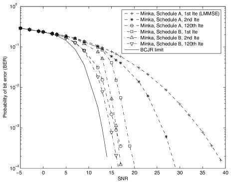
Figure 5: Bit error rate vs. SNR for uncoded binary transmission over FIR channel with transfer function $H(z)=0.227+0.46z^{-1}+0.688z^{-2}+0.46z^{-3}+0.227z^{-4}$.

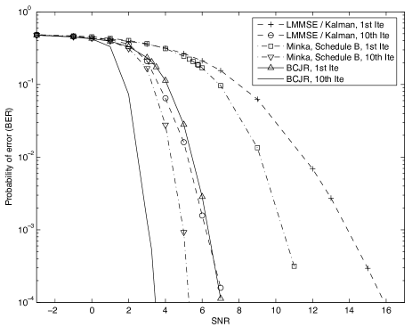
Figure 6: Bit error rate vs. SNR for coded binary transmission over FIR channel.

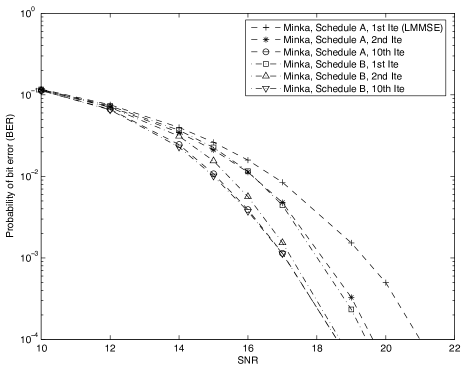
Figure 7: Bit error rate vs. SNR for uncoded binary transmission over IIR channel with transfer function $H(z)=1/(1-0.9z^{-1})$.

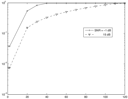
Figure 8: Good sequences for $\alpha$ vs. the iteration number $k$.

VI Conclusion

Elaborating on Minka’s work, we have formulated a general computation rule for lossy messages. An important special case is the conversion of “soft-bit” messages to Gaussian messages. In this case, the resulting Gaussian message is non-trivial even if the “soft-bit” message is neutral. By this method, the performance of a Kalman equalizer is significantly improved.

References

- [1] F. R. Kschischang, B. J. Frey, and H.-A. Loeliger, “Factor graphs and the sum-product algorithm,” IEEE Trans. Information Theory, vol. 47, pp. 498–519, Feb. 2001.
- [2] H.-A. Loeliger, “An introduction to factor graphs,” IEEE Signal Proc. Mag., Jan. 2004, pp. 28–41.
- [3] T. P. Minka, A Family of Algorithms for Approximate Bayesian Inference. PhD thesis, Massachusetts Institute of Technology (MIT), 2001.
- [4] T. P. Minka, “Expectation propagation for approximate Bayesian inference,” in Proceedings of the 17th Annual Conference on Uncertainty in Artificial Intelligence (UAI-01), vol. 17, pp. 362–369, 2001.
- [5] T. Minka and Y. Qi, “Tree-structured approximations by expectation propagation,” in Advances in Neural Information Processing Systems 16, MIT Press, 2003.
- [6] J. Dauwels, H.-A. Loeliger, P. Merkli, and M. Ostojic, “On Markov structured summary propagation and LFSR synchronization,” Proc. 42nd Allerton Conf. on Communication, Control, and Computing, (Allerton House, Monticello, Illinois), Sept. 29–Oct. 1, 2004, pp. 451–460.
- [7] H.-A. Loeliger, J. Hu, S. Korl, and Li Ping, “Gaussian message passing and related topics: an update,” Proc. 4th Int. Symp. on Turbo Codes & Related Topics, Munich, Germany, April 3–7, 2006.
- [8] J. Proakis, Digital Communications. 4th ed., McGraw-Hill, 2001.
- [9] A. Duel-Hallen and C. Heegard, “Delayed decision-feedback sequence estimation,” IEEE Trans. Communications, vol. 37, pp. 428–436, May 1989.