Path-Independent Load Balancing With Unreliable Machines

Abstract

We consider algorithms for load balancing on unreliable machines. The objective is to optimize the two criteria of minimizing the makespan and minimizing job reassignments in response to machine failures. We assume that the set of jobs is known in advance but that the pattern of machine failures is unpredictable. Motivated by the requirements of BGP routing, we consider path-independent algorithms, with the property that the job assignment is completely determined by the subset of available machines and not the previous history of the assignments. We examine first the question of performance measurement of path-independent load-balancing algorithms, giving the measure of makespan and the normalized measure of reassignments cost. We then describe two classes of algorithms for optimizing these measures against an oblivious adversary for identical machines. The first, based on independent random assignments, gives expected reassignment costs within a factor of $2$ of optimal and gives a makespan within a factor of $O(\log m/\log\log m)$ of optimal with high probability, for unknown job sizes. The second, in which jobs are first grouped into bins and at most one bin is assigned to each machine, gives constant-factor ratios on both reassignment cost and makespan, for known job sizes. Several open problems are discussed.

1 Introduction

Given a set of jobs $J=\{1\ldots n\}$ and machines $M=\{1\ldots m\}$, where each job $j$ has a size or processing time $p_{j}$, the problem of load balancing is to construct an assignment $f:J\rightarrow M$ that minimizes the makespan, defined as $C^{\max}=\max_{i\in M}\sum_{j\in f^{-1}(i)}p_{j}$.

We consider a variant of load balancing in which the set of available machines $S$ changes over time. In effect, we are solving a sequence of $P||C^{\max}$ scheduling problems where the set of jobs is fixed but the set of machines varies, and our goal is to minimize both the makespan $C^{\max}$ and the reassignment cost of moving jobs from one machine to another as new machines become available and old machines leave. As a further complication, we restrict ourselves to path-independent algorithms, those that always assign the same jobs to the same machines given a particular set $S$ despite any previous history of assignments. This restriction simplifies the description of an algorithm, since we can just present an assignment for each nonempty set of machines, but it may dramatically increase reassignment costs since we cannot take previous assignments into account. Surprisingly, we show that randomization can lower the expected reassignment cost between any two states of a path-independent algorithm to within a constant factor of optimal, while maintaining a constant approximation ratio to the optimal makespan.

This variant of load-balancing is inspired by the problem of routing among multiple network paths using the Border Gateway Protocol (BGP) [10], the de facto interdomain routing protocol of the Internet. In BGP, the global Internet is divided into multiple autonomous systems (AS). Each AS has several peering ASes, and the ASes export to its peers available routes to destination prefixes (jobs). Each AS maintains a cache (called routing information base) of currently available routes to the destinations exported by its peers, and selects routes to destinations from the routing cache using a route selection algorithm. One major objective of the route selection algorithm is load balancing among multiple peering links (machines) [15]. Figure 1 shows the standard protocol/process model of interdomain route selection of BGP [2, 13, 15].

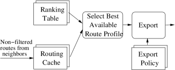
Figure 1: The protocol/process model of route selection for interdomain traffic engineering of BGP.

Because network connections are dynamic, the set of routes that are available at any time may vary. When the set of available routes changes, BGP will re-run the route selection algorithm. If the assignment of the route to a destination is changed, BGP will update its peers, and this update can propagate throughout the global Internet. Thus, it is important to minimize the number of reassignments, since they are expensive operations both in terms of bandwidth and router CPU processing [14].

Naturally, some reassignments are unavoidable: when a peering link goes down, all destination prefixes that previously used that link must be assigned elsewhere, and when new links become available, we cannot refuse to reassign destinations to them without violating our load-balancing criterion. So the number of reassignments performed by an algorithm will need to be measured against an estimate of how many reassignments are necessary, which will be obtained by considering the behavior of an ideal algorithm that maintains perfect load balance with minimal reassignment costs.

A further complication is that routers (e.g., cisco and Juniper routers) implement route selection by assigning priorities (called local preference values) to routes. This means that the assignments of destinations to peering links are unaffected by past history, a property known as path-independence. Thus, we will consider only load-balancing algorithms in which the current assignment is determined only by the current set of available machines. Furthermore, for multihomed stub ASes, such path-independent assignments can guarantee interdomain routing stability [15]. Path-independence is thus a desirable property of load-balancing algorithms for unreliable machines, motivating our study of such algorithms.

Formally, a path-independent load-balancing algorithm is just a function from $2^{M}\setminus\{\emptyset\}$ to $M^{J}$, where the argument represents the (always nonempty) set of available machines and the function value represents an assignment, with the constraint that no job is ever assigned to a machine that is not in the available set. Given such an algorithm $A$, we write $A_{S}$ for the assignment chosen by $A$ for available set $S$ and $A_{S}(j)$ for the machine to which job $j$ is assigned. With this notation, the constraint on $A$ is that $A_{S}(j)\in S$ for all $S$ and $j$.

Because the assignment of jobs to machines is determined by the set of available machines, this set completely determines the state of the system. We thus identify sets of available machines with states of the system and will refer to such sets simply as states hereafter.

1.1 Our results

The paper contains several novel contributions:

• The new problem of path-independent load balancing, motivated by practical issues in BGP routing.

• A measure of reassignment costs that takes into account the difference between small and large changes in the set of available machines. This measure is motivated and described in Section 2. We also show that standard competitive analysis techniques [12] are not useful.

• A simple algorithm, based on independent random machine preferences, that achieves low reassignment costs and $O(\log m/\log\log m)\cdot\mbox{OPT}$ makespan even with unknown job sizes. This algorithm, together with a more general class of preference-based algorithms of which it is a member, is described in Section 3.

• A more sophisticated algorithm BinHash for jobs of known sizes, based on consolidating jobs into a variable number of bins (depending on the number of available machines) and then hashing the bins. This algorithm achieves constant approximation ratios on both reassignment costs and makespan. It is described in Section 4.

Finally, in Section 5 we discuss possibilities for future work.

Because of space limitations, some proofs are sketched or moved to the appendix. Complete proofs can be found in the full paper.

1.2 Related work

It has long been known that a simple greedy algorithm [3] achieves a makespan within a factor of $2$ of optimal on identical machines. Much recent work on the problem has focused on on-line load-balancing, where jobs arrive one at a time; see [1] for an example of the current state of the art. Our work is distinguished from this work by the assumption that jobs are known, but that the set of available machines changes over time.

Kalyanasundaram and Pruhs [5, 6] have considered models of fault-tolerant scheduling for parallel computers; here the issue is that process failure prevents any job assigned to it from being completed and the goal is to maximize the total value of completed jobs subject to release time and completion time constraints. Their results are based on redundant scheduling without pre-emption and are not directly applicable to our problem.

The technique of consolidating jobs in our algorithm for known job sizes is similar to an approach taken by Sibeyn [11] for load-balancing jobs with sizes drawn from a random distribution. Sibeyn’s techniques are intended to reduce the variance in job sizes and do not have the low-reassignment-cost properties of our prefix-based method.

There has been substantial work on load-balancing mechanisms based on the power of two choices, where jobs pick two (or more) machines at random and choose the more lightly-loaded machine. (See [8] for a survey of these results.) We found through experiments that this approach, while producing excellent makespans, does not appear to yield low reassignment costs: the chains of displaced jobs that migrate to less loaded machines when a new machine becomes available are simply too long.

2 Measuring performance

We measure the performance of a path-independent load-balancing algorithm by two criteria: the makespan of $A_{S}$ for each set of available machines $S$, and the reassignment cost paid by $A$ when moving from one assignment $A_{S}$ to a different assignment $A_{T}$.

The makespan was is defined using standard notation as $C^{\max}_{A}(S)=\max_{i\in S}\sum_{j\in A_{S}^{-1}(i)}p_{j}$, the maximum total load on any one machine.

The reassignment cost $r_{A}(S,T)$ is the number of jobs that move from one machine to another between $A_{S}$ and $A_{T}$. Formally, we define $r_{A}(S,T)=|\{j|A_{S}(j)\neq A_{T}(j)\}|$. Note that sizes are not used in computing the reassignment cost; we assume that all jobs incur an equal overhead when reassigned regardless of size. Note also that reassignment cost is symmetric: $r_{A}(S,T)=r_{A}(T,S)$ for all $S$ and $T$.

An execution of a path-independent load-balancing algorithm is specified as a sequence of states $S_{0},S_{1},S_{2},\ldots$, which may or may not be finite. For a finite execution $S_{0}\ldots S_{t}$, the total reassignment cost of an algorithm $A$ is $\sum_{i=0}^{t-1}r_{A}(S_{i},S_{i+1})$. For an infinite execution, the average reassignment cost is defined as $\lim_{t\rightarrow\infty}\frac{1}{t}\sum_{i=0}^{t-1}r_{A}(s_{i},s_{i+1})$. Note that because $r_{A}$ is bounded by $n$ this limit always exists.

Because both makespan and reassignment cost are parameterized by states, an algorithm’s overall performance may depend strongly on the details of a specific execution. To be able to compare algorithms it will be useful to have summary statistics that describe the performance of an algorithm over all possible executions. Worst-case measures are of limited usefulness: the worst-case reassignment cost of any algorithm on two or more machines is $n$ jobs per step, since we may have only a single available machine at each step that alternates between steps, forcing us to always reassign jobs. Similarly, the worst-case makespan which arises when there is only one available machine does not distinguish algorithms in any way. So instead, we must consider measures that take into account the difficulty of particular executions.

We will show first that a traditional competitive analysis approach does not suffice for this purpose, and then propose an alternative method where the cost of an execution is normalized by a straw-man reference cost corresponding to the performance of a particular idealized load-balancing algorithm.

2.1 Impossibility of bicriteria-competitive algorithms

The technique of competitive analysis [12] compares the cost of a candidate on-line algorithm (which receives the input only step-by-step) in a given history against the cost of an optimal off-line algorithm (which sees the entire input in advance and is typically not computationally bounded). A candidate algorithm is said to have competitive ratio $c$ or be $c$-competitive if its cost is at most $c$ times the cost of the optimal algorithm, plus a constant.

For the path-independent load-balancing problem, we are measuring two quantities at each step: the makespan in the new state, and the reassignment cost between the old state and the new state. A natural way to apply competitive analysis to this situation might be to adopt a bicriteria approach and insist that our candidate algorithm be $(\alpha,\beta)$-competitive, where $\alpha$ bounds the ratio between the candidate’s makespan in each state and the optimal algorithm’s makespan in its corresponding state, and $\beta$ bounds the ratio between the candidate’s total reassignment cost over a finite execution and the optimal algorithm’s total reassignment cost. We show below that no such algorithm exists for any finite $\alpha$ and $\beta$ in any system with $n\geq 2$ jobs and $m\geq 2$ machines, even if the jobs have identical sizes.

Theorem 1

Let $A$ be a path-independent load-balancing algorithm for a system with $n\geq 2$ jobs and $m\geq 2$ machines. Then $A$ is not $(\alpha,\beta)$-competitive for any $\alpha$ and $\beta$.

Proof: Without loss of generality, let $m=2$ (we can always make any additional machines permanently unavailable).

Let $A$ be some candidate algorithm. We will show that $A$ is not competitive with respect to reassignment costs regardless of makespan. Let $i\in\{1,2\}$ be such that some job is assigned to machine $i$ in $A_{\{1,2\}}$; let $i^{\prime}$ be the other machine. Now consider an execution in which $S_{t}=\{1,2\}$ when $t$ is even and $S_{t}=\{i^{\prime}\}$ when $t$ is odd. Because there is some job that is assigned to machine $i$ at even times and not odd times, $A$ pays a reassignment cost of at least $1$ per step of the execution. However, an optimal $A^{*}$ that assigns all jobs to machine $i^{\prime}$ in all states pays $0$. No finite $\beta$ nor additive constant is large enough to overcome in the limit the infinite ratio between $A$ and $A^{*}$’s reassignment costs.  

2.2 Normalized reassignment costs

We define the normalized reassignment cost relative to the costs of an ideal algorithm that always maintains perfect balance. We consider first the case of $n=km!$ identical jobs, where $k$ is some integer; the $m!$ factor ensures that the jobs can be equally divided over any subset of the machines. In this case we can directly calculate the reassignment cost when moving from state $S$ to state $T$.

Theorem 2

Consider a system $m$ machines and $n=km!$ identical jobs. Let $A$ be an algorithm that assigns exactly $n/|S|$ jobs to each machine in each state $S$. Then the number of reassignments performed by $A$ going from $S$ to $T$ is at least

$$r^{*}(S,T)=n\cdot\left(1-\frac{|S\cap T|}{\max\left(|S|,|T|\right)}\right).$$ (1)

Proof: Consider the set of jobs assigned to machines in $S\setminus T$ by $A_{S}$; since $A$ assigns exactly $n/|S|$ jobs to each machine in $S\setminus T$, there are $n\cdot|S\setminus T|/|S|$ such jobs total. All of these jobs must be reassigned going from $S$ to $T$.

Conversely, any job assigned to a machine in $T\setminus S$ by $A_{T}$ must also have been reassigned going from $S$ to $T$. Though these two sets of jobs may overlap, $A$ must reassign at least

$$n\cdot\max\left(\frac{|S\setminus T|}{|S|},\frac{|T\setminus S|}{|T|}\right) = n\cdot\max\left(\frac{|S\setminus(S\cap T)|}{|S|},\frac{|T\setminus(S\cap T)|}{|T|}\right)$$

$$= n\cdot\max\left(1-\frac{|S\cap T|}{|S|},1-\frac{|S\cap T|}{|T|}\right)$$

$$= n\cdot\left(1-\frac{|S\cap T|}{\max\left(|S|,|T|\right)}\right).$$

 

We will take $r^{*}$ as the ideal reassignment cost, and measure the reassignment cost of any particular algorithm $A$ as the maximum over all $S$ and $T$ of the ratio of its reassignment cost $r_{A}(S,T)$ to $r^{*}(S,T)$.

A justification for this approach is that the $r^{*}$ lower bound continues to hold in expectation for any algorithm—regardless of whether it distributes jobs evenly or not—provided the machine names are randomly permuted before the algorithm is used and such renaming is undone afterwards. This fact is formally stated in the following theorem. The random permutation of machine names, which is easily implemented by an oblivious adversary, prevents an algorithm from getting lucky by placing all of its jobs on machines that stay available in both $S$ and $T$.

Theorem 3

For any algorithm $A$ that maps states to assignments, choose a permutation $\rho$ uniformly at random. Let $\rho^{-1}A\rho$ be the algorithm that constructs an assignment for $S$ by applying $A$ to $\rho S$ and then undoing the machine renaming. Then the algorithm $\rho^{-1}A\rho$ reassigns at least $n\cdot\left(1-\frac{|S\cap T|}{\max(|S|,|T|)}\right)$ jobs in expectation when moving from state $S$ to state $T$.

The proof is given in Appendix A.

3 Preference-based algorithms

A preference-based algorithm is one in which each job is assigned a permutation of the machines (which may depend on the set of other jobs), and always moves to the first available machine in its permutation. We can think of the operation of a preference-based algorithm as choosing for each job $j$ and state $S$ the machine $i$ in $S$ that minimizes $\sigma_{j}(i)$, where $\sigma_{j}$ is the permutation for job $j$.

We consider first the reassignment costs of preference-based algorithms in general and then the makespan of the simple preference-based algorithm where each $\sigma_{j}$ is a random permutation.

3.1 Reassignment costs

Preference-based algorithms have the desirable property that they achieve close to the minimum reassignment cost against an oblivious adversary, provided the preferences are permuted randomly before the algorithm is used. This fact is stated formally in the following theorem.

Theorem 4

For each job $j$, let $\sigma_{j}$ be a permutation of the machines. Choose a permutation $\rho$ uniformly at random. Then the preference-based algorithm using preferences $\sigma_{j}\rho$ reassigns an expected $n\cdot\left(1-\frac{|S\cap T|}{|S\cup T|}\right)$ jobs when moving from state $S$ to state $T$.

Proof: Fix some particular job $j$. Going from $S$ to $T$, job $j$ stays put just in case $\min_{i\in S}\sigma_{j}\rho(i)=\min_{i\in T}\sigma_{j}\rho(i)$. This occurs precisely when $\min_{i\in S\cup T}\sigma_{j}\rho(i)$ is achieved by some $i$ in $S\cap T$, i.e. when neither $S$ nor $T$ provides a machine that $j$ prefers to the best machine in their intersection. Since $\sigma_{j}\rho$ is a random permutation, the probability that $j$ does not move is thus precisely $|S\cap T|/|S\cup T|$. The expected number of moves is obtained by taking one minus this probability and summing over all $n$ jobs.  

Corollary 5

For any preference-based algorithm $A$ and any states $S$ and $T$, $\mathop{\rm E}\nolimits[r_{A}(S,T)]\leq 2r^{*}(S,T)$, where $r^{*}$ is defined as in Theorem 2.

Sketch of Proof: Follows from showing that $\mathop{\rm E}\nolimits[r_{A}(S,T)]=n\cdot\left(1-\frac{|S\cap T|}{|S\cup T|}\right)\leq 2n\cdot\max\left(\frac{|S\setminus T|}{|S|},\frac{|T\setminus S|}{|T|}\right)=2r^{*}(S,T)$.  

3.2 Makespan for random preferences

A typical case of preference-based algorithms is the random preference algorithm, in which a fixed random permutation of machines is picked independently for each job as its preference list.

This randomization implicitly subsumes the random permutation of machine names assumed in Corollary 5; thus the corollary applies and random preferences yield an expected $2r^{*}(S,T)$ reassignments going from state $S$ to $T$. For identical jobs, the makespan of random preference when all machines are available is $\Theta(\log m/\log\log m)\cdot\mbox{OPT}$ w.h.p. for $n=m$, and is $(n/m)+\Theta\left(\sqrt{(n/m)\log m}\right)=\mbox{OPT}\cdot\left(1+\Theta\left(\sqrt{(m/n)\log m}\right)\right)$ w.h.p. for large $n$, using standard balls-in-bins results (e.g. [9]). Reducing the number of available machines effectively replaces $m$ with $|S|$ in the latter expression.

If the jobs are not identical, we can still argue that the makespan is $O(\log m/\log\log m)\cdot\mbox{OPT}$, using a generalization to weighted balls of the usual balls-in-bins results. Here we assume that we have a bound on both the weight of the largest ball and the expected weight of the balls assigned to any one bin. These quantities are both bounded by the optimal makespan.

Lemma 6

Let $n$ balls with non-negative weights $w_{1},w_{2},\ldots w_{n}$ be distributed independently and uniformly at random into $b\leq m$ bins. Let $W=\max\left(\max(w_{i}),\frac{1}{b}\sum_{i=1}^{n}w_{i}\right).$ Let $X$ be the maximum over all bins of the total weight of the balls in that bin. Then for any fixed $c$, there exists a constant $k$ such that $X\leq kW\lg m/\lg\lg m$ with probability $1-o(m^{-c})$.

The proof, a straightforward application of characteristic functions, is given in Appendix B. Applying Lemma 6 to the random-preference algorithm yields:

Theorem 7

The random-preference algorithm achieves a makespan of $O(\log m/\log\log m)\cdot\mbox{OPT}$ with high probability for any fixed set $S$ of available machines.

Proof: Apply Lemma 6 with $b=|S|$ and $W=\mbox{OPT}$.  

Note that the probability that Theorem 7 fails is polynomial in $m$, while the number of possible subsets of available machines is exponential. So it is possible that the makespan for some particular subset $S$ is much worse. This is not a problem if we assume an oblivious adversary, but may become one if a more powerful adversary can choose $S$ after determining the algorithm’s preference lists—which it can do by observing the algorithm’s behavior.

4 Algorithm based on binning and hashing

In this section, we introduce an algorithm called BinHash which achieves constant approximation ratios for both makespan and reassignment costs. Unlike the random-preference algorithm of Section 3.2, the makespan bound is deterministic and holds in all states. (The reassignment cost bound is still probabilistic.)

The algorithm is based on the observation that if the number of jobs $n\leq\alpha|S|$ for some constant load factor $\alpha$, we can get low reassignment costs and (trivially) optimal makespan by assigning each job to the first empty machine on its preference list. This process—the hashing step—is structurally equivalent to hashing with open addressing, and the number of reassignments caused by adding or removing a job is bounded by the length of chains in the corresponding hashing algorithm, which is a constant for fixed $\alpha$.

However, since we cannot assume $n\leq\alpha|S|$ in general, we add an initial binning step where jobs are assigned to $\max(1,\left\lfloor{\alpha|S|}\right\rfloor)$ bins, which are then hashed to machines. The binning step sorts jobs by size, and then assigns each job to the bin whose index, expressed in binary, is the longest available suffix of the index of the job. This is a form of round-robin assignment that, by spreading the jobs roughly uniformly among the bins, guarantees a constant-factor approximation of the optimal makespan. At the same time, the number of jobs that move when the number of bins changes is small, since in addition to guaranteeing an even spread by size the binning procedure also guarantees an even spread by job count, and adding or deleting a bin only splits some existing bin or combines two previous bins.

We now give a formal definition of the algorithm. Given $n$ jobs with sizes $p_{0}\geq p_{1}\geq\cdots\geq p_{n-1}$, and a set $S\in 2^{[m]}/\{\emptyset\}$ of available machines, BinHash computes an assignment of $n$ jobs to the machines in $S$ in two stages:

1. Binning stage: Let $b=\max\{\lfloor\alpha|S|\rfloor,1\}$, where $\alpha\in(0,1)$ is the load factor parameter of the algorithm. Assign the $n$ jobs to $b$ bins by calling the function $\mathcal{B}(\{p_{0},p_{1},\ldots,p_{n-1}\},b)\mapsto\langle B^{(b)}_{0},B^{(b)}_{1},\ldots,B^{(b)}_{b-1}\rangle$, where $B^{(b)}_{i}$ is computed by

   $$A_{i} \leftarrow \{j=i+k\cdot 2^{\lceil\log{(i+1)}\rceil}\mid k\geq 0\wedge 0\leq j\leq n-1\}$$

   $$B^{(b)}_{i} \leftarrow A_{i}-\bigcup_{l=i+1}^{b-1}B^{(b)}_{l}$$

   for $i=b-1,b-2,\ldots,0$.

   In other words, each bin $B^{(b)}_{i}$ gets precisely those jobs whose binary expansions include the binary expansion of $i$ as a suffix, provided there are no higher-numbered bins that capture them first. It is immediate from the definition of $B^{(b)}_{i}$ that every jobs is assigned to exactly one bin.

2. Hashing stage: The bins are now assigned to the machines in $S$ in order by a uniform hashing function $\mathcal{H}(i,S)$, where for each $i$ from $0$ to $\left\lfloor{\alpha m}\right\rfloor$, bin $i$ is hashed to the first machine in a fixed random permutation of all $m$ machines that is in $S$ and not occupied by a lower-numbered bin.

We now show that the BinHash algorithm achieves low makespan. This follows from the even distribution of the sizes of the bins and the fact that at most one bin is assigned to each machine.

Lemma 8

Assuming that the optimal makespan of assigning $n$ jobs to $|S|$ machines is OPT, then

$$\max_{0\leq i\leq b-1}|B_{i}^{(b)}|\leq\frac{4n}{\alpha|S|}$$

and

$$\max_{0\leq i\leq b-1}{\sum_{j\in B_{i}^{(b)}}p_{j}}\leq(1+2/\alpha)\cdot\mbox{OPT}$$

for $b=\max\{\lfloor\alpha|S|\rfloor,1\}$.

The proof is given in Appendix C.

To show low reassignment costs, we must take into account both reassignments caused by moving bins (when a machine leaves or becomes available) and reassignments caused by moving jobs between bins. The former is bounded by the fact that the number of jobs in each bin is roughly equal. The latter requires an analysis of the hashing step. To simplify the argument, we consider first only the case where a single machine becomes unavailable. The case of a new machine becoming available has the same cost by symmetry, and we will show later in Theorem 10 that the cost of larger transformations can be expressed in terms of these two cases.

Lemma 9

For $T\subset S$, and $|T|=|S|-1$, the algorithm BinHash reassigns at most an expected $\frac{4(2-\alpha)n}{\alpha(1-\alpha)|S|}$ jobs when moving from state $S$ to state $T$.

Proof: The total reassignments can be upper bounded by the sum of reassignments caused by binning and the reassignments caused by bin displacements due to hashing.

According to the definition of binning stage in BinHash, it is easy to verify that for any $b\geq 1$,

$$B^{(b)}_{b-2^{\lfloor\log{b}\rfloor}} = B^{(b+1)}_{b-2^{\lfloor\log{b}\rfloor}}\cup B^{(b+1)}_{b}$$

$$B^{(b)}_{i} = B^{(b+1)}_{i}\mbox{\qquad for }i\neq b-2^{\lfloor\log{b}\rfloor}.$$

Thus the reduction of the last bin is the only case for the reassignments caused by binning process.

For the single machine in $S\backslash T$, there might be a bin $i$ assigned to it in state $S$. When the state changes from $S$ to $T$, bin $i$ will be assigned to some other machine in $T$ by the hashing step. This may lead to a recursive displacement of further bins with larger index than $i$. Since the placement of bin $i$ in $T$ is uncorrelated with the preferences of later bins, the number of such displacements can be bounded by the maximum number of bin displacements caused by inserting an additional bin with an random index into state $T$’s assignment.

Suppose that $n<m$, and let $\Delta(n,m,i)$ denote the expected displacements led by inserting an object with index $i\geq 0$ to a hash table with $m$ slots and $n$ objects by uniform hashing. It is obvious that all objects with priority $h<i$ will not move, therefore it is equivalent to assume that all such objects and their slots are not available to our analysis, thus with probability $\frac{n-i}{m-i}$ object $i$ hits a slot which is occupied by object $i^{\prime}$ where $i^{\prime}>i$, and then triggers an expected $\Delta(n,m,i^{\prime})$ displacements led by inserting object $i^{\prime}$.

$$\Delta(n,m,i)=\left\{\begin{array}[]{lc}1&i=n\\ 1+\frac{n-i}{m-i}\Delta(n,m,i^{\prime})\\ \mbox{\quad\qquad for some }i^{\prime}>i&\mbox{ \emph{o.w.}}.\end{array}\right.$$

By induction, it is easy to show that $\Delta(n,m,i)\leq 1/(1-\frac{n}{m})$ for all $i\geq 0$.

Applying this to the bin assignment, we have at most $\Delta(b-1,|S|-1,i)$ displacements of bins, where $b=\max\{\lfloor\alpha|S|\rfloor,1\}$, therefore,

$$\Delta(b-1,|S|-1,i)\leq\frac{1}{1-\alpha}.$$

The total reassignment costs in terms of jobs is thus bounded from above by $(1+1/(1-\alpha))\max_{0\leq i\leq b-1}|B_{i}^{(b)}|\leq\frac{4(2-\alpha)n}{\alpha(1-\alpha)|S|}$.  

We now combine the results in Lemmas 8 and 9 to obtain the full result:

Theorem 10

The following claims hold for any constant $0<\alpha<1$:

For any $n>0$ and state $S$, assuming that the optimal makespan of assigning $n$ jobs to $|S|$ machines is OPT, then the makespan of the assignment obtained by running BinHash with the $n$ jobs on $S$ is within $(1+2/\alpha)\cdot OPT$.

For any states $S$ and $T$, the expected number of reassignments performed by BinHash going from $S$ to $T$,

$$\mathop{\rm E}\nolimits[r_{B}(S,T)]\leq 2\left(1+\frac{4(2-\alpha)}{\alpha(1-\alpha)}\right)\cdot r^{*}(S,T),$$

where the expectation is taken over the randomness of uniform hashing, and $r^{*}$ is defined as in Theorem 2.

Proof: Since only one bin is assigned to each machine, the upper bound on makespan follows directly from Lemma 8.

For the state transition from $S$ to $T$, where $T\subset S$, according to Lemma 9, we have that

$$\mathop{\rm E}\nolimits[r_{B}(S,T)] \leq \min\left\{n,\frac{4(2-\alpha)n}{\alpha(1-\alpha)}\left(\frac{1}{|S|}+\frac{1}{|S|-1}+\ldots+\frac{1}{|T|+1}\right)\right\}$$

$$\leq \min\left\{n,\frac{4(2-\alpha)n}{\alpha(1-\alpha)}\ln\frac{|S|}{|T|}\right\}$$

$$\leq \left(1+\frac{4(2-\alpha)}{\alpha(1-\alpha)}\right)(1-|T|/|S|)n$$

$$= \left(1+\frac{4(2-\alpha)}{\alpha(1-\alpha)}\right)\cdot r^{*}(S,T).$$

For a general $S$ and $T$, we have that

$$\mathop{\rm E}\nolimits[r_{B}(S,T)] \leq \mathop{\rm E}\nolimits[r_{B}(S,S\cap T)]+\mathop{\rm E}\nolimits[r_{B}(T,s\cap T)]$$

$$\leq \left(1+\frac{4(2-\alpha)}{\alpha(1-\alpha)}\right)(r^{*}(S,S\cap T)+r^{*}(T,S\cap T))$$

$$\leq 2\left(1+\frac{4(2-\alpha)}{\alpha(1-\alpha)}\right)\cdot r^{*}(S,T).$$

 

It is not hard to show that the coefficient on reassignment costs is minimized at $\alpha=2-\sqrt{2}\approx 0.59\ldots$. Here the reassignment costs are bounded by Theorem 2 at approximately $48.6\cdot r^{*}$ and the makespan at $(3+\sqrt{2})\cdot\mbox{OPT}\approx 4.142\cdot\mbox{OPT}$. There are a number of loose inequalities in the proof of Theorem 2, and we believe that a more careful analysis would show that the correct minimum coefficient on reassignment costs is closer to $12$ in most cases.

It is also worth noting that the makespan coefficient $1+2/\alpha$ can be reduced somewhat by increasing $\alpha$. However, this dramatically increases the reassignment costs as $\alpha$ approaches $1$, and the makespan bound never drops below $3\cdot\mbox{OPT}$, which is not much better than the bound for $\alpha=2-\sqrt{2}$. However, it is not out of the question that a more sophisticated algorithm could achieve higher utilization of the available machines without blowing up the reassignment costs.

5 Conclusions and future work

We have described a new problem of path-independent load balancing for unreliable machines, where the goal is to minimize makespan while simultaneously minimizing the cost of reassigning jobs from one machine to another subject to the constraint that assignments cannot depend on the previous history. We have also obtained some initial results showing that it is possible to achieve constant approximation ratios to both the optimal makespan and optimal reassignment costs.

However, much work still needs to be done. The proven constant approximation ratios for the BinHash algorithm—particularly for makespan—are still quite high, and it would be useful to have an algorithm with better constants.

The assumption of identical machines is a strong one. It is not clear whether our results can be generalized to the case of uniform machines (where different machines have different capacities) or to the even more general case of nonuniform machines (where different jobs may have different effective sizes on different machines). This last case may be particularly important in interdomain routing, as particular flows may be forbidden from traveling over certain pipes by contractual requirements or security concerns.

Finally, we have made very generous assumptions about the nature of the jobs and the nature of the adversary. It would be interesting to determine whether it is possible to solve path-independent load balancing with jobs that vary over time or with a more powerful adversary that can observe and respond to the algorithm’s actions.

Appendix A Proof of Theorem 3

Fix some particular job $j$. Let $A_{S}(j)$ be the machine to which $A$ assigns job $j$ in state $S$. Note that $A_{S}(j)\in S$. Observe that:

• For any $\langle U,V\rangle$ where $|U|=|S|$, $|V|=|T|$ and $|U\cap V|=|S\cap T|$, there exists some permutation $\rho$ such that $\langle U,V\rangle=\langle\rho S,\rho T\rangle$.

• There are ${m\choose|S|}{|S|\choose|S\cap T|}{m-|S|\choose|T|-|S\cap T|}$ equivalence classes after applying permutations to $\langle S,T\rangle$, each of which contains $|S\cap T|!(|S|-|S\cap T|)!(|T|-|S\cap T|)!(m-|S\cup T|)!$ permutations. We denote this value as $e(S,T)$.

• Fix $S$ and $T$. For any $\rho S$, the number of $\rho T$ which contain $A_{\rho S}(j)$, i.e., $|\{\rho T\mid A_{\rho S}(j)\in\rho T\}|$ equals ${|S|-1\choose|S\cap T|-1}{m-|S|\choose|T|-|S\cap T|}$.

Then the probability that job $j$ stays while the state going from $S$ to $T$

$$\Pr\rho[A_{\rho S}(j)=A_{\rho T}(j)] = \frac{1}{m!}\sum_{\rho}|\{\rho\mid A_{\rho S}(j)=A_{\rho T}(j)\}|$$

$$= \frac{1}{m!}\sum_{\rho S}|\{\rho T\mid A_{\rho S}(j)=A_{\rho T}(j)\}|\cdot e(S,T)$$

$$\leq \frac{1}{m!}\sum_{\rho S}|\{\rho T\mid A_{\rho S}(j)\in\rho T)\}|\cdot e(S,T)$$

$$= \frac{1}{m!}\sum_{\rho S}{|S|-1\choose|S\cap T|-1}{m-|S|\choose|T|-|S\cap T|}\cdot e(S,T)$$

$$= \frac{|S\cap T|}{|S|}.$$

Symmetrically,

$$\Pr\rho[A_{\rho S}(j)=A_{\rho T}(j)] \leq \frac{|S\cap T|}{|T|}.$$

Therefore, we have $\Pr\rho[A_{\rho S}(j)=A_{\rho T}(j)]\leq\frac{|S\cap T|}{\max(|S|,|T|)}$. The probability that job $j$ is reassigned from $S$ to $T$ is thus lower bounded by $(1-\frac{|S\cap T|}{\max(|S|,|T|)})$. The expected total cost is obtained by summing over all $n$ jobs.

Appendix B Proof of Lemma 6

The proof is a straightforward generalization of the usual argument using characteristic functions for for $n=m$ identical balls.

Let $p=1/b$, $q=1-p$, and $\alpha>0$. Let $X_{i}$ be a random variable representing the weight that the $i$-th ball contributes to some particular bin. Let $S=\sum_{i}X_{i}$. Then

$$\mathop{\rm E}\nolimits\left[e^{\alpha S}\right] = \mathop{\rm E}\nolimits\left[\prod_{i}e^{\alpha X_{i}}\right]$$

$$= \prod_{i}\left(qe^{0}+pe^{\alpha w_{i}}\right)$$

$$\leq \prod_{i}\left(1+pe^{\alpha w_{i}}\right)$$

$$\leq \prod_{i}\exp\left(pe^{\alpha w_{i}}\right)$$

$$= \exp\left(p\sum_{i}e^{\alpha w_{i}}\right).$$

Now apply Markov’s inequality to get

$$\Pr\left[S>t\right] = \Pr\left[e^{\alpha S}>e^{\alpha t}\right]$$

$$< \exp\left(p\sum_{i}e^{\alpha w_{i}}\right)-\exp(\alpha t)$$

$$= \exp\left(p\sum_{i}e^{\alpha w_{i}}-\alpha t\right).$$

We now choose the $w_{i}$ to maximize this quantity subject to the given constraints $w_{i}\leq W$ and $\sum_{i}w_{i}\leq bW$. Observe that this is equivalent to maximizing $\sum_{i}e^{\alpha w_{i}}$. Since $e^{\alpha w_{i}}$ is convex, this is maximized subject to the sum constraint by setting $w_{i}=W$ for $i=1\ldots b$ and $w_{i}=0$ elsewhere. We thus have

$$\Pr\left[S>t\right] < \exp\left(p\sum_{i}e^{\alpha w_{i}}-\alpha t\right)$$

$$\leq \exp\left(pbe^{\alpha W}-\alpha t\right)$$

$$= \exp\left(e^{\alpha W}-\alpha t\right).$$

It is not hard to show that the best choice for $\alpha$ is $\ln(t/W)/W$, giving

$$\Pr\left[S>t\right] < \exp\left(e^{\ln(t/W)}-(t/W)\ln(t/W)\right)$$

$$= \exp\left((t/W)-(t/W)\ln(t/W)\right).$$

$$= \exp\left((t/W)(1-\ln(t/W)\right).$$

Finally, set $t/W=k\ln m/\ln\ln m$ to get

$$\Pr\left[S>t\right] < \exp\left(\frac{k\ln m}{\ln\ln m}\left(1-\ln k-\ln\ln m+\ln\ln\ln m\right)\right)$$

$$= m^{\left\{k\left(\frac{1-\ln k}{\ln\ln m}-1+\frac{\ln\ln\ln m}{\ln\ln m}\right)\right\}}$$

$$= m^{-k(1-o(1))}.$$

So the probability that any of the $b$ bins exceeds $kW\ln m/\ln\ln m$ is at most $bm^{-k(1-o(1))}\leq m^{1-k(1-o(1))}$, which is $o\left(m^{-c}\right)$ for sufficiently large $k$.

Appendix C Proof of Lemma 8

By noting that $B_{i}^{(b)}$ contains all such $j$ whose longest available suffix in binary expansion is $i$, it is easy to verify that,

$$B_{i}^{(b)}\subseteq\{j=i+k\cdot 2^{\lfloor\log{b}\rfloor}\mid k\geq 0\wedge 0\leq j\leq n-1\}.$$ (2)

Therefore, for any $0\leq i\leq b-1$

$$|B_{i}^{(b)}|\leq\lfloor\frac{n}{2^{\lfloor\log{b}\rfloor}}\rfloor\leq\frac{2n}{b}\leq\frac{4n}{\alpha|S|}.$$

As for the loads of bins, note that $OPT\geq\max\{p_{0},\frac{1}{|S|}\sum_{j=0}^{n-1}p_{j}\}$. According to (2) and the non-increasing order of $p_{j}$, we have that, for each $0\leq i\leq b-1$,

$$\sum_{j\in B_{i}^{(b)}}p_{j} \leq \sum_{k\geq 0}p_{i+k\cdot 2^{\lfloor\log{b}\rfloor}}$$

$$= p_{i}+\sum_{k\geq 1}\frac{1}{2^{\lfloor\log{b}\rfloor}}\cdot 2^{\lfloor\log{b}\rfloor}\cdot p_{i+k\cdot 2^{\lfloor\log{b}\rfloor}}$$

$$\leq p_{0}+\sum_{k\geq 1}\frac{1}{2^{\lfloor\log{b}\rfloor}}\sum_{t=0}^{-1+2^{\lfloor\log{b}\rfloor}}p_{i+k\cdot 2^{\lfloor\log{b}\rfloor}-t}$$

$$\leq p_{0}+\frac{1}{2^{\lfloor\log{b}\rfloor}}\sum_{j=0}^{n-1}p_{j}$$

$$\leq p_{0}+\frac{2}{b}\sum_{j=0}^{n-1}p_{j}$$

$$\leq p_{0}+\frac{2}{\alpha|S|}\sum_{j=0}^{n-1}p_{j}$$

$$\leq (1+2/\alpha)\cdot OPT.$$

References

- [1] S. Albers. On randomized online scheduling. In Proceedings of the 34th ACM Symposium on Theory of Computing, pages 134–143, 2002.
- [2] M. Caesar and J. Rexford. BGP routing policies in ISP networks. IEEE Network Magazine, special issue on Interdomain Routing, Nov/Dev 2006.
- [3] R. Graham. Bounds for certain multi-processing anomalies. Bell Systems Technical Journal, 45:1563–1581, 1966.
- [4] R. Graham, E. Lawler, J. Lenstra, and A. Rinnooy Kan. Optimization and approximation in deterministic sequencing and scheduling: A survey. Annals of Discrete Mathematics, 5:287–326, 1979.
- [5] B. Kalyanasundaram and K. Pruhs. Fault-tolerant real-time scheduling. Algorithmica, 28(1):125–144, 2000.
- [6] B. Kalyanasundaram and K. Pruhs. Fault-tolerant scheduling. SIAM J. Comput., 34(3):697–719, 2005.
- [7] J. Y.-T. Leung, editor. Handbook of Scheduling: Algorithms, Models, and Performance Analysis. CRC Press, 2004.
- [8] M. Mitzenmacher, A. W. Richa, and R. Sitaraman. The power of two random choices: A survey of techniques and results. In S. Rajasekaran, P. Pardalos, J. Reif, and J. Rolim, editors, Handbook of Randomized Computing, volume I, pages 255–305. Springer, 2001.
- [9] M. Raab and A. Steger. ”Balls into bins”—a simple and tight analysis. In Randomization and Approximation Techniques in Computer Science, Second International Workshop, RANDOM’98, Barcelona, Spain, October 8-10, 1998, Proceedings, volume 1518 of Lecture Notes in Computer Science, pages 159–170. Springer, 1998.
- [10] Y. Rekhter and T. Li. A Border Gateway Protocol 4 (BGP-4), RFC 1771, Mar. 1995.
- [11] J. F. Sibeyn. The sum of weighted balls. Technical Report RUU-CS-91-37, Department of Computer Science, Utrecht University, 1991.
- [12] D. D. Sleator and R. E. Tarjan. Amortized efficiency of list update and paging rules. Communications of the ACM, 28(2):202–208, Feb. 1985.
- [13] J. L. Sobrinho. Network routing with path vector protocols: Theory and applications. In Proceedings of ACM SIGCOMM ’03, Karlsruhe, Germany, Aug. 2003.
- [14] L. Subramanian, M. Caesar, C. T. Ee, M. Handley, M. Mao, S. Shenker, and I. Stoica. HLP: A next-generation interdomain routing protocol. In Proceedings of ACM SIGCOMM ’05, Philadelphia, PA, Aug. 2005.
- [15] H. Wang, H. Xie, Y. R. Yang, L. E. Li, Y. Liu, and A. Silberschatz. Stable egress route selection for interdomain traffic engineering: Model and analysis. In Proceedings of the 13th International Conference on Network Protocols (ICNP) ’05, Boston, MA, Nov. 2005.