Sparse Matrix Implementation in Octave

Abstract

This paper discusses the implementation of the sparse matrix support with Octave. It address the algorithms that have been used, their implementation, including examples of using sparse matrices in scripts and in dynamically linked code. The octave sparse functions the compared with their equivalent functions with Matlab, and benchmark timings are calculated.

1 Introduction

The size of mathematical problems that can be treated at any particular time is generally limited by the available computing resources. Both the speed of the computer and its available memory place limitations on the problem size.

There are many classes of mathematical problems which give rise to matrices, where a large number of the elements are zero. In this case it makes sense to have a special matrix type to handle this class of problems where only the non-zero elements of the matrix are stored. Not only does this reduce the amount of memory to store the matrix, but it also means that operations on this type of matrix can take advantage of the a-priori knowledge of the positions of the non-zero elements to accelerate their calculations. A matrix type that stores only the non-zero elements is generally called sparse.

This article address the implementation of sparse matrices within Octave [1, 2], including their storage, creation, fundamental algorithms used, their implementations and the basic operations and functions implemented for sparse matrices. Benchmarking of Octave’s implementation of sparse operations compared to their equivalent in Matlab [3] are given and their implications discussed. Furthermore, the method of using sparse matrices with Octave oct-files is discussed.

In order to motivate this use of sparse matrices, consider the image of an automobile crash simulation as shown in Figure 1. This image is generated based on ideas of DIFFCrash [4] – a software package for the stability analysis of crash simulations. Physical bifurcations in automobile design and numerical instabilities in simulation packages often cause extremely sensitive dependencies of simulation results on even the smallest model changes. Here, a prototypic extension of DIFFCrash uses octave’s sparse matrix functions (and large computers with lots of memory) to produce these results.

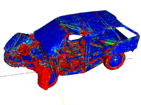
Fig. 1: Image of automobile crash simulation, blue regions indicate rigid-body behaviour. Image courtesy of BMW and Fraunhofer Institute SCAI.

2 Basics

2.1 Storage of Sparse Matrices

It is not strictly speaking necessary for the user to understand how sparse matrices are stored. However, such an understanding will help to get an understanding of the size of sparse matrices. Understanding the storage technique is also necessary for those users wishing to create their own oct-files.

There are many different means of storing sparse matrix data. What all of the methods have in common is that they attempt to reduce the complexity and storage given a-priori knowledge of the particular class of problems that will be solved. A good summary of the available techniques for storing sparse matrix is given by Saad [5]. With full matrices, knowledge of the point of an element of the matrix within the matrix is implied by its position in the computers memory. However, this is not the case for sparse matrices, and so the positions of the non-zero elements of the matrix must equally be stored.

An obvious way to do this is by storing the elements of the matrix as triplets, with two elements being their position in the array (rows and column) and the third being the data itself. This is conceptually easy to grasp, but requires more storage than is strictly needed.

The storage technique used within Octave is the compressed column format. In this format the position of each element in a row and the data are stored as previously. However, if we assume that all elements in the same column are stored adjacent in the computers memory, then we only need to store information on the number of non-zero elements in each column, rather than their positions. Thus assuming that the matrix has more non-zero elements than there are columns in the matrix, we win in terms of the amount of memory used.

In fact, the column index contains one more element than the number of columns, with the first element always being zero. The advantage of this is a simplication in the code, in that their is no special case for the first or last columns. A short example, demonstrating this in C is.

⬇

for (j = 0; j < nc; j++)

for (i = cidx (j); i < cidx(j+1); i++)

printf (”Element (%i,%i) is %d\n”,

ridx(i), j, data(i));

A clear understanding might be had by considering an example of how the above applies to an example matrix. Consider the matrix

1	2	0	0
0	0	0	3
0	0	0	4

The non-zero elements of this matrix are

$$(1,1) = 1$$

$$(1,2) = 2$$

$$(2,4) = 3$$

$$(3,4) = 4$$

This will be stored as three vectors $cidx$, $ridx$ and $data$, representing the column indexing, row indexing and data respectively. The contents of these three vectors for the above matrix will be

$$cidx = [0,1,2,2,4]$$

$$ridx = [0,0,1,2]$$

$$data = [1,2,3,4]$$

Note that this is the representation of these elements with the first row and column assumed to start at zero, while in Octave itself the row and column indexing starts at one. With the above representation, the number of elements in the $i^{th}$ column is given by $cidx(i+1)-cidx(i)$.

Although Octave uses a compressed column format, it should be noted that compressed row formats are equally possible. However,in the context of mixed operations between mixed sparse and dense matrices, it makes sense that the elements of the sparse matrices are in the same order as the dense matrices. Octave stores dense matrices in column major ordering, and so sparse matrices are equally stored in this manner.

A further constraint on the sparse matrix storage used by Octave is that all elements in the rows are stored in increasing order of their row index, which makes certain operations faster. However, it imposes the need to sort the elements on the creation of sparse matrices. Having unordered elements is potentially an advantage in that it makes operations such as concatenating two sparse matrices together easier and faster, however it adds complexity and speed problems elsewhere.

2.2 Creating Sparse Matrices

There are several means to create sparse matrices

• Returned from a function: There are many functions that directly return sparse matrices. These include speye, sprand, spdiag, etc.

• Constructed from matrices or vectors: The function sparse allows a sparse matrix to be constructed from three vectors representing the row, column and data. Alternatively, the function spconvert uses a three column matrix format to allow easy importation of data from elsewhere.

• Created and then filled: The function sparse or spalloc can be used to create an empty matrix that is then filled by the user

• From a user binary program: The user can directly create the sparse matrix within an oct-file.

There are several functions that return specific sparse matrices. For example the sparse identity matrix is often needed. It therefore has its own function to create it as speye$(n)$ or speye$(r,c)$, which creates an $n$-by-$n$ or $r$-by-$c$ sparse identity matrix.

Another typical sparse matrix that is often needed is a random distribution of random elements. The functions sprand and sprandn perform this for uniform and normal random distributions of elements. They have exactly the same calling convention, where sprand$(r,c,d)$, creates an $r$-by-$c$ sparse matrix with a density of filled elements of $d$.

Other functions of interest that directly creates a sparse matrices, are spdiag or its generalization spdiags, that can take the definition of the diagonals of the matrix and create the sparse matrix that corresponds to this. For example

⬇

s = spdiag (sparse(randn(1,n)),-1);

creates a sparse $(n+1)$-by-$(n+1)$ sparse matrix with a single diagonal defined.

The recommended way for the user to create a sparse matrix, is to create two vectors containing the row and column index of the data and a third vector of the same size containing the data to be stored. For example

⬇

function x = foo (r, j)

idx = randperm (r);

x = ([zeros(r-2,1); rand(2,1)])(idx);

endfunction

ri = [];

ci = [];

d = [];

for j=1:c

dtmp = foo (r, j);

idx = find (dtmp != 0.);

ri = [ri; idx];

ci = [ci; j*ones(length(idx),1)];

d = [d; dtmp(idx)];

endfor

s = sparse (ri, ci, d, r, c);

creates an $r$-by-$c$ sparse matrix with a random distribution of 2 elements per row. The elements of the vectors do not need to be sorted in any particular order as Octave will sort them prior to storing the data. However, pre-sorting the data will make the creation of the sparse matrix faster.

The function spconvert takes a three or four column real matrix. The first two columns represent the row and column index, respectively, and the third and four columns, the real and imaginary parts of the sparse matrix. The matrix can contain zero elements and the elements can be sorted in any order. Adding zero elements is a convenient way to define the size of the sparse matrix. For example

⬇

s = spconvert ([1 2 3 4; 1 3 4 4; 1 2 3 0]’)

Compressed Column Sparse (rows=4, …

cols=4, nnz=3)

(1 , 1) -> 1

(2 , 3) -> 2

(3 , 4) -> 3

An example of creating and filling a matrix might be

⬇

k = 5;

nz = r * k;

s = spalloc (r, c, nz)

for j = 1:c

idx = randperm (r);

s (:, j) = [zeros(r - k, 1); …

rand(k, 1)] (idx);

endfor

It should be noted, that due to the way that the Octave assignment functions are written that the assignment will reallocate the memory used by the sparse matrix at each iteration of the above loop. Therefore the spalloc function ignores the nz argument and does not preassign the memory for the matrix. Therefore, code using the above structure should be vectorized to minimize the number of assignments and reduce the number of memory allocations.

The above problem can be avoided in oct-files. However, the construction of a sparse matrix from an oct-file is more complex than can be discussed in this brief introduction, and you are referred to section 6, to have a full description of the techniques involved.

2.3 Sparse Functions in Octave

An important consideration in the use of the sparse functions of Octave is that many of the internal functions of Octave, such as diag, can not accept sparse matrices as an input. The sparse implementation in Octave therefore uses the dispatch function to overload the normal Octave functions with equivalent functions that work with sparse matrices. However, at any time the sparse matrix specific version of the function can be used by explicitly calling its function name.

The table below lists all of the sparse functions of Octave together (with possible future extensions that are currently unimplemented, listed last). Note that in this specific sparse forms of the functions are typically the same as the general versions with a sp prefix. In the table below, and the rest of this article the specific sparse versions of the functions are used.

• Generate sparse matrices: spalloc, spdiags, speye, sprand, sprandn, (sprandsym)

• Sparse matrix conversion: full, sparse, spconvert, spfind

• Manipulate sparse matrices issparse, nnz, nonzeros, nzmax, spfun, spones, spy,

• Graph Theory: etree, etreeplot, gplot, treeplot, (treelayout)

• Sparse matrix reordering: ccolamd, colamd, colperm, csymamd, symamd, randperm, (dmperm, symrcm)

• Linear algebra: matrix_type, spchol, spcholinv, spchol2inv, spdet, spinv, spkron, splchol, splu, (condest, eigs, normest, sprank, svds, spaugment, spqr)

• Iterative techniques: luinc, (bicg, bicgstab, cholinc, cgs, gmres, lsqr, minres, pcg, pcr, qmr, symmlq)

• Miscellaneous: spparms, symbfact, spstats, spprod, spcumsum, spsum, spsumsq, spmin, spmax, spatan2, spdiag

In addition all of the standard Octave mapper functions (ie. basic math functions that take a single argument) such as abs, etc can accept sparse matrices. The reader is referred to the documentation supplied with these functions within Octave itself for further details.

2.4 Sparse Return Types

The two basic reasons to use sparse matrices are to reduce the memory usage and to not have to do calculations on zero elements. The two are closely related and the computation time might be proportional to the number of non-zero elements or a power of the number of non-zero elements depending on the operator or function involved.

Therefore, there is a certain density of non-zero elements of a matrix where it no longer makes sense to store it as a sparse matrix, but rather as a full matrix. For this reason operators and functions that have a high probability of returning a full matrix will always return one. For example adding a scalar constant to a sparse matrix will almost always make it a full matrix, and so the example

⬇

speye(3) + 0

1 0 0

0 1 0

0 0 1

returns a full matrix as can be seen. Additionally all sparse functions test the amount of memory occupied by the sparse matrix to see if the amount of storage used is larger than the amount used by the full equivalent. Therefore speye(2) * 1 will return a full matrix as the memory used is smaller for the full version than the sparse version.

As all of the mixed operators and functions between full and sparse matrices exist, in general this does not cause any problems. However, one area where it does cause a problem is where a sparse matrix is promoted to a full matrix, where subsequent operations would re-sparsify the matrix. Such cases are rare, but can be artificially created, for example (fliplr(speye(3)) + speye(3)) - speye(3) gives a full matrix when it should give a sparse one. In general, where such cases occur, they impose only a small memory penalty.

There is however one known case where this behavior of Octave’s sparse matrices will cause a problem. That is in the handling of the spdiag function. Whether spdiag returns a sparse or full matrix depends on the type of its input arguments. So

⬇

a = diag (sparse([1,2,3]), -1);

should return a sparse matrix. To ensure this actually happens, the sparse function, and other functions based on it like speye, always returns a sparse matrix, even if the memory used will be larger than its full representation.

2.5 Finding out Information about Sparse Matrices

There are a number of functions that allow information concerning sparse matrices to be obtained. The most basic of these is issparse that identifies whether a particular Octave object is in fact a sparse matrix.

Another very basic function is nnz that returns the number of non-zero entries there are in a sparse matrix, while the function nzmax returns the amount of storage allocated to the sparse matrix. Note that Octave tends to crop unused memory at the first opportunity for sparse objects. There are some cases of user created sparse objects where the value returned by nzmaz will not be the same as nnz, but in general they will give the same result. The function spstats returns some basic statistics on the columns of a sparse matrix including the number of elements, the mean and the variance of each column.

When solving linear equations involving sparse matrices Octave determines the means to solve the equation based on the type of the matrix as discussed in section 3. Octave probes the matrix type when the div ($/$) or ldiv ($\backslash$) operator is first used with the matrix and then caches the type. However the matrix_type function can be used to determine the type of the sparse matrix prior to use of the div or ldiv operators. For example

⬇

a = tril (sprandn(1024, 1024, 0.02), -1) …

+ speye(1024);

matrix_type (a);

ans = Lower

show that Octave correctly determines the matrix type for lower triangular matrices. matrix_type can also be used to force the type of a matrix to be a particular type. For example

⬇

a = matrix_type (tril (sprandn (1024, …

1024, 0.02), -1) + speye(1024), ’Lower’);

This allows the cost of determining the matrix type to be avoided. However, incorrectly defining the matrix type will result in incorrect results from solutions of linear equations, and so it is entirely the responsibility of the user to correctly identify the matrix type

There are several graphical means of finding out information about sparse matrices. The first is the spy command, which displays the structure of the non-zero elements of the matrix, as can be seen in Figure 4. More advanced graphical information can be obtained with the treeplot, etreeplot and gplot commands.

One use of sparse matrices is in graph theory, where the interconnections between nodes is represented as an adjacency matrix [6]. That is, if the $i$-th node in a graph is connected to the $j$-th node. Then the $ij$-th node (and in the case of undirected graphs the $ji$-th node) of the sparse adjacency matrix is non-zero. If each node is then associated with a set of co-ordinates, then the gplot command can be used to graphically display the interconnections between nodes.

As a trivial example of the use of gplot, consider the example

⬇

A = sparse([2,6,1,3,2,4,3,5,4,6,1,5],

[1,1,2,2,3,3,4,4,5,5,6,6],1,6,6);

xy = [0,4,8,6,4,2;5,0,5,7,5,7]’;

gplot(A,xy)

which creates an adjacency matrix A where node 1 is connected to nodes 2 and 6, node 2 with nodes 1 and 3, etc. The co-ordinates of the nodes is given in the n-by-2 matrix xy. The output of the gplot command can be seen in Figure 2

Fig. 2: Simple use of the gplot command as discussed in Section 2.5.

The dependences between the nodes of a Cholesky factorization can be calculated in linear time without explicitly needing to calculate the Cholesky factorization by the etree command. This command returns the elimination tree of the matrix and can be displayed grapically by the command treeplot(etree(A)) if A is symmetric or treeplot(etree(A+A’)) otherwise.

2.6 Mathematical Considerations

The attempt has been made to make sparse matrices behave in exactly the same manner as their full counterparts. However, there are certain differences between full and sparse behavior and with the sparse implementations in other software tools.

Firstly, the ./ and .^∧ operators must be used with care. Consider what the examples

$$s = speye(4);$$

$$a1 = s.^{\wedge}2;$$

$$a2 = s.^{\wedge}s;$$

$$a3 = s.^{\wedge}-2;$$

$$a4 = s./2;$$

$$a5 = 2./s;$$

$$a6 = s./s;$$

will give. The first example of $s$ raised to the power of 2 causes no problems. However $s$ raised element-wise to itself involves a a large number of terms 0 .^∧ 0 which is 1. Therefore s .^∧ s is a full matrix.

Likewise s .^∧ -2 involves terms terms like 0 .^∧ -2 which is infinity, and so s .^∧ -2 is equally a full matrix.

For the ./ operator s ./ 2 has no problems, but 2 ./ s involves a large number of infinity terms as well and is equally a full matrix. The case of s ./ s involves terms like 0 ./ 0 which is a NaN and so this is equally a full matrix with the zero elements of $s$ filled with NaN values. The above behavior is consistent with full matrices, but is not consistent with sparse implementations in Matlab [7]. If the user requires the same behavior as in Matlab then for example for the case of 2 ./ s then appropriate code is

⬇

function z = f(x), z = 2 ./ x; endfunction

spfun (@f, s);

and the other examples above can be implemented similarly.

A particular problem of sparse matrices comes about due to the fact that as the zeros are not stored, the sign-bit of these zeros is equally not stored. In certain cases the sign-bit of zero is important [8]. For example

⬇

a = 0 ./ [-1, 1; 1, -1];

b = 1 ./ a

-Inf Inf

Inf -Inf

c = 1 ./ sparse (a)

Inf Inf

Inf Inf

To correct this behavior would mean that zero elements with a negative sign-bit would need to be stored in the matrix to ensure that their sign-bit was respected. This is not done at this time, for reasons of efficiency, and so the user is warned that calculations where the sign-bit of zero is important must not be done using sparse matrices.

In general any function or operator used on a sparse matrix will result in a sparse matrix with the same or a larger number of non-zero elements than the original matrix. This is particularly true for the important case of sparse matrix factorizations. The usual way to address this is to reorder the matrix, such that its factorization is sparser than the factorization of the original matrix. That is the factorization of $LU=PSQ$ has sparser terms $L$ and $U$ than the equivalent factorization $LU=S$.

Several functions are available to reorder depending on the type of the matrix to be factorized. If the matrix is symmetric positive-definite, then symamd or csymamd should be used. Otherwise colamd or ccolamd should be used. For completeness the reordering functions colperm and randperm are also available.

As an example, consider the ball model which is given as an example in the EIDORS project [9, 10], as shown in Figure 3. The structure of the original matrix derived from this problem can be seen with the command spy(A), as seen in Figure 4.

Fig. 3: Geometry of FEM model of phantom ball model from EIDORS project [9, 10]

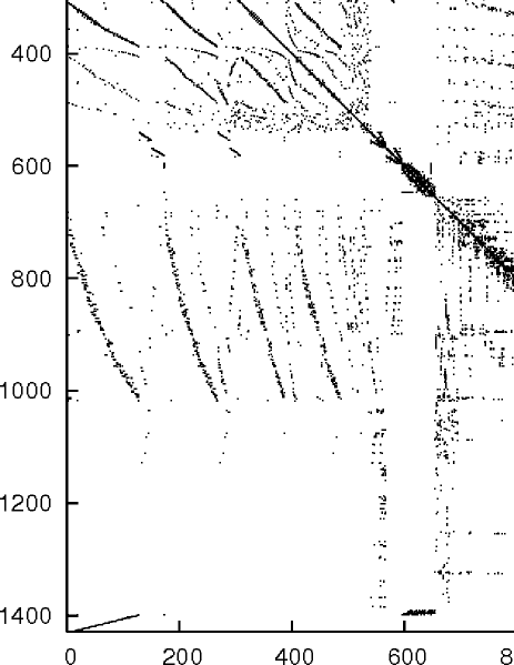
Fig. 4: Structure of the sparse matrix derived from EIDORS phantom ball model [9, 10]

The standard LU factorization of this matrix, with row pivoting can be obtained by the same command that would be used for a full matrix. This can be visualized with the command [l, u, p] = lu(A); spy(l+u); as seen in Figure 5. The original matrix had 17825 non-zero terms, while this LU factorization has 531544 non-zero terms, which is a significant level of fill in of the factorization and represents a large overhead in working with this matrix.

The appropriate sparsity preserving permutation of the original matrix is given by colamd and the factorization using this reordering can be visualized using the command q = colamd(A); [l, u, p] = lu(A(:,q)); spy(l+u). This gives 212044 non-zero terms which is a significant improvement.

Furthermore, the underlying factorization software updates its estimate of the optimal sparsity preserving reordering of the matrix during the factorization, so can return an even sparser factorization. In the case of the LU factorization this might be obtained with a fourth return argument as [l, u, p, q] = lu(A); spy(l+u). This factorization has 143491 non-zero terms, and its structure can be seen in Figure 6.

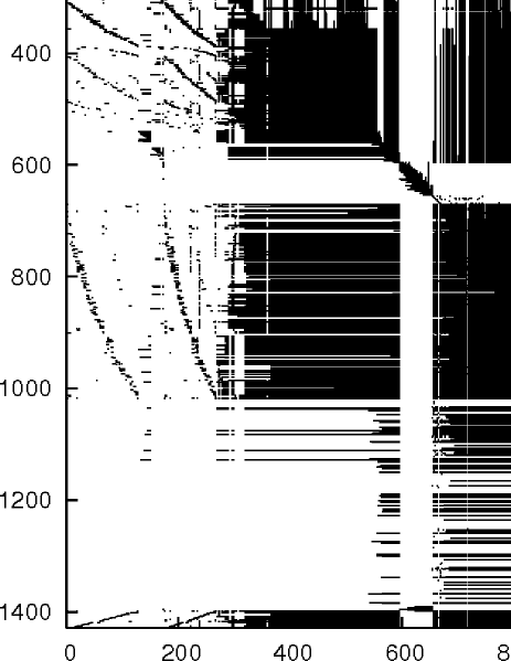
Fig. 5: Structure of the un-permuted LU factorization of EIDORS ball problem

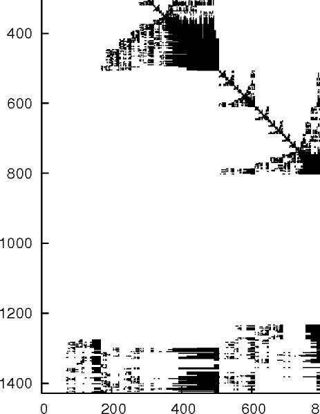
Fig. 6: Structure of the permuted LU factorization of EIDORS ball problem

Finally, Octave implicitly reorders the matrix when using the div ($/$) and ldiv ($\backslash$) operators, and so no the user does not need to explicitly reorder the matrix to maximize performance.

3 Linear Algebra on Sparse Matrices

Octave includes a polymorphic solver for sparse matrices, where the exact solver used to factorize the matrix, depends on the properties of the sparse matrix itself. Generally, the cost of determining the matrix type is small relative to the cost of factorizing the matrix itself, but in any case the matrix type is cached once it is calculated, so that it is not re-determined each time it is used in a linear equation.

Linear equations are solved using the following selection tree

1. If the matrix is not square go to 9.

2. If the matrix is diagonal, solve directly and go to 9

3. If the matrix is a permuted diagonal, solve directly taking into account the permutations. Go to 9

4. If the matrix is banded and if the band density is less than that given by spparms (”bandden”) continue, else go to 5.

   1. If the matrix is tridiagonal and the right-hand side is not sparse continue, else go to 4b.

      1. If the matrix is hermitian, with a positive real diagonal, attempt Cholesky factorization using Lapack xPTSV.

      2. If the above failed, or the matrix is not hermitian, use Gaussian elimination with pivoting using Lapack xGTSV, and go to 9.

   2. If the matrix is hermitian with a positive real diagonal, attempt a Cholesky factorization using Lapack xPBTRF.

   3. if the above failed or the matrix is not hermitian with a positive real diagonal use Gaussian elimination with pivoting using Lapack xGBTRF, and go to 9.

5. If the matrix is upper or lower triangular perform a sparse forward or backward substitution, and go to 9

6. If the matrix is a upper triangular matrix with column permutations or lower triangular matrix with row permutations, perform a sparse forward or backward substitution, and go to 9

7. If the matrix is hermitian with a real positive diagonal, attempt a sparse Cholesky factorization using CHOLMOD [11].

8. If the sparse Cholesky factorization failed or the matrix is not hermitian, perform LU factorization using UMFPACK [12].

9. If the matrix is not square, or any of the previous solvers flags a singular or near singular matrix, find a minimum norm solution.

The band density is defined as the number of non-zero values in the band divided by the number of values in the band. The banded matrix solvers can be entirely disabled by using spparms to set bandden to 1 (i.e. spparms (”bandden”, 1)).

The QR solver factorizes the problem with a Dulmage-Mendhelsohn [13], to seperate the problem into blocks that can be treated as over-determined, multiple well determined blocks, and a final over-determined block. For matrices with blocks of strongly connectted nodes this is a big win as LU decomposition can be used for many blocks. It also significantly improves the chance of finding a solution to ill-conditioned problems rather than just returning a vector of NaN’s.

All of the solvers above, can calculate an estimate of the condition number. This can be used to detect numerical stability problems in the solution and force a minimum norm solution to be used. However, for narrow banded, triangular or diagonal matrices, the cost of calculating the condition number is significant, and can in fact exceed the cost of factoring the matrix. Therefore the condition number is not calculated in these case, and octave relies on simplier techniques to detect sinular matrices or the underlying LAPACK code in the case of banded matrices.

The user can force the type of the matrix with the matrix_type function. This overcomes the cost of discovering the type of the matrix. However, it should be noted incorrectly identifying the type of the matrix will lead to unpredictable results, and so matrix_type should be used with care.

4 Benchmarking of Octave Sparse Matrix Implementation

It is a truism that all benchmarks should be treated with care. The speed of a software package is determined by a large number of factors, including the particular problem treated and the configuration of the machine on which the benchmarks were run. Therefore the benchmarks presented here should be treated as indicative of the speed a user might expect.

That being said we attempt to examine the speed of several fundamental operators for use with sparse matrices. These being the addition (+), multiplication (*) and left-devision ($\backslash$) operators. The basic test code used to perform these tests is given by

⬇

time = 0;

n = 0;

while (time < tmin || n < nrun)

clear a, b;

a = sprand (order, order, density);

t = cputime ();

b = a OP a;

time = time + cputime () - t;

n = n + 1;

end

time = time / n;

where nrun was 5, tmin was 1 second and OP was either +, or *. The left-division operator poses particular problems for benchmarking that will be discussed later.

Although the cputime function only has a resolution of 0.01 seconds, running the command multiple times and limited by the minimum run time of tmin seconds allows this precision to be extended. Running the above code for various matrix orders and densities results in the summary of execution times as seen in Table 1.

Order	Den-	Execution Time for Operator (sec)
	sity	Matlab		Octave
		+	*	+	*
500	1e-02	0.00049	0.00250	0.00039	0.00170
500	1e-03	0.00008	0.00009	0.00022	0.00026
500	1e-04	0.00005	0.00007	0.00020	0.00024
500	1e-05	0.00004	0.00007	0.00021	0.00015
500	1e-06	0.00006	0.00007	0.00020	0.00021
1000	1e-02	0.00179	0.02273	0.00092	0.00990
1000	1e-03	0.00021	0.00027	0.00029	0.00042
1000	1e-04	0.00011	0.00013	0.00023	0.00026
1000	1e-05	0.00012	0.00011	0.00028	0.00023
1000	1e-06	0.00012	0.00010	0.00021	0.00022
2000	1e-02	0.00714	0.23000	0.00412	0.07049
2000	1e-03	0.00058	0.00165	0.00055	0.00135
2000	1e-04	0.00032	0.00026	0.00026	0.00033
2000	1e-05	0.00019	0.00020	0.00022	0.00026
2000	1e-06	0.00018	0.00018	0.00024	0.00023
5000	1e-02	0.05100	3.63200	0.02652	0.95326
5000	1e-03	0.00526	0.03000	0.00257	0.01896
5000	1e-04	0.00076	0.00083	0.00049	0.00074
5000	1e-05	0.00051	0.00051	0.00031	0.00043
5000	1e-06	0.00048	0.00055	0.00028	0.00026
10000	1e-02	0.22200	24.2700	0.10878	6.55060
10000	1e-03	0.02000	0.30000	0.01022	0.18597
10000	1e-04	0.00201	0.00269	0.00120	0.00252
10000	1e-05	0.00094	0.00094	0.00047	0.00074
10000	1e-06	0.00110	0.00098	0.00039	0.00055
20000	1e-03	0.08286	2.65000	0.04374	1.71874
20000	1e-04	0.00944	0.01923	0.00490	0.01500
20000	1e-05	0.00250	0.00258	0.00092	0.00149
20000	1e-06	0.00189	0.00161	0.00058	0.00121
50000	1e-04	0.05500	0.39400	0.02794	0.28076
50000	1e-05	0.00823	0.00877	0.00406	0.00767
50000	1e-06	0.00543	0.00610	0.00154	0.00332

Table 1: Benchmark of basic operators on Matlab R14sp2 against Octave 2.9.5, on a Pentium 4M 1.6GHz machine with 1GB of memory.

The results for the small low density problems in Table 1 are interesting (cf. Matrix order of 500, with densities lower than 1e-03), as they seem to indicate that there is a small incompressible execution time for both Matlab and Octave. This is probably due to the overhead associated with the parsing of the language and the calling of the underlying function responsible for the operator. On the test machine this time was approximately 200 $\mu$s for Octave for both operators, while for Matlab this appears to be 70 and 40 $\mu$s for the * and + operators respectively. So in this class of problems Matlab outperforms Octave for both operators. However, when the matrix order or density increases it can be seen that Octave significantly out-performs Matlab for both operators.

When considering the left-division operator, we can not use randomly created matrices. The reason is that the fill-in, or rather the potential to reduce the fill-in with appropriate matrix re-ordering, during matrix factorization is determined by the structure of the matrix imposed by the problem it represents. As random matrices have no structure, factorization of random matrices results in extremely large levels of matrix fill-in, even with matrix re-ordering. Therefore, to benchmark the left-division ($\backslash$) operator, we have selected a number of test matrices that are publicly available [14], and modify the benchmark code as

⬇

time = 0;

n = 0;

while (time < tmin || n < nrun)

clear a, b;

load test.mat % Get matrix ’a’

x = ones(order,1);

t = cputime ();

b = a \ x;

time = time + cputime () - t;

n = n + 1;

end

time = time / n;

All the the matrices in the University of Florida Sparse Matrix [14] that met the following criteria were used

• Has real or complex data available, and not just the structure,

• Has between 10,000 and 1,000,000 non-zero element,

• Has equal number of rows and columns,

• The solution did not require more than 1GB of memory, to avoid issues with memory.

When comparing the benchmarks for the left-division operator it must be considered that the matrices in the collection used represent an arbitrary sampling of the available sparse matrix problems. It is therefore difficult to treat the data in aggregate, and so we present the raw data below so that the reader might compare the benchmark for a particular matrix class that interests them.

The performance of the Matlab and Octave left-division operators is affected by the spparms function. In particular the density of terms in a banded matrix that is needed to force the solver to use the LAPACK banded solvers rather than the generic solvers is determined by the command spparms(’bandden’,val). The default density of 0.5 was used for both Matlab and Octave.

Five classes of problems were represented in the matrices treated. These are

• Banded positive definite and factorized with the LAPACK xPBTRF function,

• General banded matrix and factorized with the LAPACK xGBTRF function,

• Positive definite and treated by the Cholesky solvers of Matlab and Octave,

• Sparse LU decomposition with UMFPACK, and

• Singular matrices that were treated via QR decomposition.

Also, it should be noted that the LAPACK solvers, and dense BLAS kernels of the UMFPACK and CHOLMOD solvers were accelerated using the ATLAS [15] versions of the LAPACK and BLAS functions. The exact manner in which the ATLAS library is compiled might have an affect on the performance, and therefore the benchmarks might measure the relative performance of the different versions of ATLAS rather than the performance of Octave and Matlab. To avoid this issue Octave was forced to use the Matlab ATLAS libraries with the use of the Unix LD_PRELOAD command.

Matrix	Order	NNZ	S†	Execution Time		Matrix	Order	NNZ	S†	Execution Time
				for Operator (sec)						for Operator (sec)
				Matlab	Octave					Matlab	Octave
Bai/dw1024	2048	10114	8	0.05000	0.03585	HB/nos3	960	15844	7	0.04417	0.01050
Boeing/bcsstm38	8032	10485	9	0.04333	0.02490	Bai/rbsa480	480	17088	8	0.05000	0.02905
Zitney/extr1	2837	10967	8	0.03846	0.02052	Bai/rbsb480	480	17088	8	0.04545	0.02575
vanHeukelum/cage8	1015	11003	8	0.07714	0.05039	Hollinger/g7jac010	2880	18229	8	0.18000	0.13538
FIDAP/ex32	1159	11047	8	0.04333	0.02354	Hollinger/g7jac010sc	2880	18229	8	0.15600	0.13778
Sandia/adder_dcop_05	1813	11097	8	0.03000	0.01693	Mallya/lhr01	1477	18427	8	0.05667	0.02982
Sandia/adder_dcop_04	1813	11107	8	0.02889	0.01680	HB/bcsstk09	1083	18437	7	0.05778	0.02012
Sandia/adder_dcop_03	1813	11148	8	0.03059	0.01690	FIDAP/ex21	656	18964	8	0.03846	0.02390
Sandia/adder_dcop_01	1813	11156	8	0.02941	0.01670	Wang/wang1	2903	19093	8	0.23400	0.14818
Sandia/init_adder1	1813	11156	8	0.02889	0.01667	Wang/wang2	2903	19093	8	0.22800	0.14798
Sandia/adder_dcop_06	1813	11224	8	0.02833	0.01693	Brethour/coater1	1348	19457	9	0.19000	0.07413
Sandia/adder_dcop_07	1813	11226	8	0.02889	0.01670	HB/bcsstm12	1473	19659	7	0.07000	0.01037
Sandia/adder_dcop_10	1813	11232	8	0.03000	0.01670	Hamm/add32	4960	19848	8	0.06500	0.03869
Sandia/adder_dcop_09	1813	11239	8	0.02889	0.01706	Bai/olm5000	5000	19996	4d	0.00463	0.00546
Sandia/adder_dcop_08	1813	11242	8	0.03118	0.01696	Gset/G57	5000	20000	8	0.15800	0.09332
Sandia/adder_dcop_11	1813	11243	8	0.02889	0.01693	HB/sherman3	5005	20033	8	0.12200	0.07285
Sandia/adder_dcop_13	1813	11245	8	0.02889	0.01751	Shyy/shyy41	4720	20042	8	0.08833	0.05149
Sandia/adder_dcop_19	1813	11245	8	0.02889	0.01693	Bai/rw5151	5151	20199	8	0.21600	0.13078
Sandia/adder_dcop_44	1813	11245	8	0.02889	0.01713	Oberwolfach/t3dl_e	20360	20360	4c	0.00105	0.00327
Sandia/adder_dcop_02	1813	11246	8	0.03059	0.01769	Boeing/bcsstm35	30237	20619	9	0.09333	0.05429
Sandia/adder_dcop_12	1813	11246	8	0.02889	0.01606	Grund/bayer08	3008	20698	8	0.09667	0.05766
Sandia/adder_dcop_14	1813	11246	8	0.02889	0.01683	Grund/bayer05	3268	20712	8	0.02125	0.00998
Sandia/adder_dcop_15	1813	11246	8	0.02833	0.01676	Grund/bayer06	3008	20715	8	0.10000	0.05799
Sandia/adder_dcop_16	1813	11246	8	0.02778	0.01683	HB/sherman5	3312	20793	8	0.09333	0.05259
Sandia/adder_dcop_17	1813	11246	8	0.02889	0.01727	Wang/swang1	3169	20841	8	0.08500	0.04817
Sandia/adder_dcop_18	1813	11246	8	0.02889	0.01703	Wang/swang2	3169	20841	8	0.08500	0.04808
Sandia/adder_dcop_20	1813	11246	8	0.02889	0.01680	Grund/bayer07	3268	20963	8	0.01923	0.01010
Sandia/adder_dcop_21	1813	11246	8	0.02778	0.01686	HB/bcsstm13	2003	21181	9	0.10200	0.06949
Sandia/adder_dcop_22	1813	11246	8	0.03000	0.01700	Bomhof/circuit_2	4510	21199	8	0.04250	0.02395
Sandia/adder_dcop_23	1813	11246	8	0.03059	0.01690	Boeing/bcsstk34	588	21418	7	0.09333	0.01539
Sandia/adder_dcop_24	1813	11246	8	0.02889	0.01727	TOKAMAK/utm1700b	1700	21509	8	0.08143	0.05009
Sandia/adder_dcop_25	1813	11246	8	0.03000	0.01693	HB/bcsstk10	1086	22070	7	0.11800	0.00826
Sandia/adder_dcop_26	1813	11246	8	0.03000	0.01700	HB/bcsstm10	1086	22092	8	0.14000	0.02008
Sandia/adder_dcop_27	1813	11246	8	0.02889	0.01713	Hamrle/Hamrle2	5952	22162	8	0.11000	0.06299
Sandia/adder_dcop_28	1813	11246	8	0.02889	0.01680	FIDAP/ex33	1733	22189	7	0.06875	0.01205
Sandia/adder_dcop_29	1813	11246	8	0.02789	0.01680	HB/saylr4	3564	22316	8	0.18000	0.11338
Sandia/adder_dcop_30	1813	11246	8	0.02889	0.01680	FIDAP/ex22	839	22460	8	0.04154	0.02234
Sandia/adder_dcop_31	1813	11246	8	0.02889	0.01693	Zitney/hydr1	5308	22680	8	0.09000	0.04972
Sandia/adder_dcop_32	1813	11246	8	0.02941	0.01693	HB/sherman2	1080	23094	8	0.08500	0.05379
Sandia/adder_dcop_33	1813	11246	8	0.02833	0.01710	Gset/G40	2000	23532	8	1.05000	0.90126
Sandia/adder_dcop_34	1813	11246	8	0.02833	0.01690	Gset/G39	2000	23556	8	1.03400	0.82907
Sandia/adder_dcop_35	1813	11246	8	0.02889	0.01693	Gset/G42	2000	23558	8	1.06200	0.85347
Sandia/adder_dcop_36	1813	11246	8	0.02889	0.01683	Gset/G41	2000	23570	8	0.99200	0.83307
Sandia/adder_dcop_37	1813	11246	8	0.03000	0.01693	FIDAP/ex29	2870	23754	8	0.08143	0.04754
Sandia/adder_dcop_38	1813	11246	8	0.02737	0.01703	Boeing/bcsstm34	588	24270	8	0.05556	0.06349
Sandia/adder_dcop_39	1813	11246	8	0.02778	0.01789	FIDAP/ex25	848	24369	8	0.05000	0.02679
Sandia/adder_dcop_40	1813	11246	8	0.02889	0.01738	HB/mcfe	765	24382	8	0.06500	0.03473
Sandia/adder_dcop_41	1813	11246	8	0.02941	0.01686	Gset/G56	5000	24996	9	4.56000	5.42238
Sandia/adder_dcop_42	1813	11246	8	0.03059	0.01693	Shen/shermanACa	3432	25220	8	0.14200	0.11558
Sandia/adder_dcop_43	1813	11246	8	0.03118	0.01696	Grund/meg4	5860	25258	8	0.09667	0.05359
Sandia/adder_dcop_45	1813	11246	8	0.02941	0.01713	HB/lns_3937	3937	25407	8	0.18800	0.12218
Sandia/adder_dcop_46	1813	11246	8	0.02889	0.01700	HB/lnsp3937	3937	25407	8	0.19800	0.12238
Sandia/adder_dcop_47	1813	11246	8	0.02833	0.01713	Boeing/msc01050	1050	26198	7	0.09167	0.01307
Sandia/adder_dcop_48	1813	11246	8	0.02889	0.01703	HB/bcsstk21	3600	26600	7	0.10800	0.03778
Sandia/adder_dcop_49	1813	11246	8	0.02941	0.01713	Bai/qc324	324	26730	4d	0.02125	0.02182
Sandia/adder_dcop_50	1813	11246	8	0.02889	0.01670	FIDAP/ex2	441	26839	8	0.02889	0.01900
Sandia/adder_dcop_51	1813	11246	8	0.02889	0.01670	Gset/G62	7000	28000	8	0.24600	0.15178
Sandia/adder_dcop_52	1813	11246	8	0.02833	0.01673	Hohn/fd12	7500	28462	8	0.21600	0.14018
Sandia/adder_dcop_53	1813	11246	8	0.02889	0.01693	Grund/bayer03	6747	29195	8	0.12600	0.07170
Sandia/adder_dcop_54	1813	11246	8	0.02833	0.01683	Bai/rdb5000	5000	29600	8	0.18400	0.11418
Sandia/adder_dcop_55	1813	11246	8	0.02889	0.01693	DRIVCAV/cavity06	1182	29675	8	0.05667	0.03111
Sandia/adder_dcop_56	1813	11246	8	0.02889	0.01686	DRIVCAV/cavity08	1182	29675	8	0.05778	0.02982
Sandia/adder_dcop_57	1813	11246	8	0.02941	0.01673	Lucifora/cell1	7055	30082	8	0.20000	0.11298
Sandia/adder_dcop_58	1813	11246	8	0.02889	0.01686	Lucifora/cell2	7055	30082	8	0.20000	0.11338
Sandia/adder_dcop_59	1813	11246	8	0.02833	0.01686	HB/bcsstk26	1922	30336	7	0.13600	0.01638
Sandia/adder_dcop_60	1813	11246	8	0.03000	0.01690	FIDAP/ex4	1601	31849	8	0.09333	0.05009
Sandia/adder_dcop_61	1813	11246	8	0.02889	0.01696	Gset/G65	8000	32000	8	0.28600	0.18157
Sandia/adder_dcop_62	1813	11246	8	0.02889	0.01676	HB/plat1919	1919	32399	7	0.12800	0.02359
Sandia/adder_dcop_63	1813	11246	8	0.02889	0.01686	DRIVCAV/cavity05	1182	32632	8	0.06500	0.03433
Sandia/adder_dcop_64	1813	11246	8	0.02889	0.01686	Rajat/rajat03	7602	32653	8	0.16800	0.09932
Sandia/adder_dcop_65	1813	11246	8	0.02889	0.01683	DRIVCAV/cavity07	1182	32702	8	0.05778	0.03206
Sandia/adder_dcop_66	1813	11246	8	0.02889	0.01696	DRIVCAV/cavity09	1182	32702	8	0.06111	0.03206
Sandia/adder_dcop_67	1813	11246	8	0.02833	0.01670	Grund/poli_large	15575	33033	8	0.04333	0.02625
Sandia/adder_dcop_68	1813	11246	8	0.02889	0.01686	HB/gemat12	4929	33044	8	0.09167	0.05109
Sandia/adder_dcop_69	1813	11246	8	0.02941	0.01676	HB/gemat11	4929	33108	8	0.09333	0.05099
HB/watt_1	1856	11360	8	0.06000	0.03649	Hollinger/jan99jac020	6774	33744	8	0.24200	0.15978
HB/watt_2	1856	11550	8	0.07000	0.04015	Hollinger/jan99jac020sc	6774	33744	8	0.24800	0.16877
Grund/bayer09	3083	11767	8	0.03714	0.01969	HB/bcsstk11	1473	34241	7	0.11000	0.01710
Bai/rdb2048	2048	12032	8	0.05889	0.03486	HB/bcsstk12	1473	34241	7	0.11200	0.01716
Rajat/rajat12	1879	12818	8	0.03125	0.01726	Gset/G61	7000	34296	9	11.28600	13.77691
HB/bcsstk08	1074	12960	7	0.05556	0.01723	Boeing/msc00726	726	34518	7	0.19200	0.05269
MathWorks/Pd	8081	13036	8	0.01786	0.00994	Bomhof/circuit_1	2624	35823	8	0.11200	0.05309
Hamm/add20	2395	13151	8	0.04500	0.02485	Gset/G66	9000	36000	8	0.33000	0.21097
Zitney/radfr1	1048	13299	8	0.02684	0.01375	Mallya/lhr02	2954	36875	8	0.11800	0.06399
HB/orsreg_1	2205	14133	8	0.10000	0.05932	Oberwolfach/t2dal_a	4257	37465	8	0.13800	0.09099
Sandia/adder_trans_01	1814	14579	8	0.03643	0.02104	FIDAP/ex27	974	37652	8	0.07143	0.03814
Sandia/adder_trans_02	1814	14579	8	0.03400	0.02000	Gset/G10	800	38352	8	0.53800	0.42993
Bai/pde2961	2961	14585	8	0.07000	0.03807	Gset/G6	800	38352	8	0.53600	0.42454
HB/bcsstm25	15439	15439	4c	0.00075	0.00248	Gset/G7	800	38352	8	0.54600	0.44433
Boeing/bcsstm37	25503	15525	9	0.06875	0.02833	Gset/G8	800	38352	8	0.60000	0.42714

Table 2: Benchmark of left-division operator on Matlab R14sp2 against Octave 2.9.5, on a Pentium 4M 1.6GHz machine with 1GB of memory. † The solver used for the problem, as given in section 3

Matrix	Order	NNZ	S†	Execution Time		Matrix	Order	NNZ	S†	Execution Time
				for Operator (sec)						for Operator (sec)
				Matlab	Octave					Matlab	Octave
Gset/G9	800	38352	8	0.61400	0.42054	Zitney/rdist1	4134	94408	8	0.16600	0.08565
Boeing/nasa1824	1824	39208	8	0.21000	0.06166	Averous/epb1	14734	95053	8	0.56600	0.34515
Nasa/nasa1824	1824	39208	7	0.16000	0.02590	GHS_indef/linverse	11999	95977	4d	0.01378	0.01686
Gset/G27	2000	39980	8	2.88000	2.85177	IBM_Austin/coupled	11341	97193	8	0.44000	0.23836
Gset/G28	2000	39980	8	3.33200	3.14972	Langemyr/comsol	1500	97645	8	0.15200	0.08449
Gset/G29	2000	39980	8	2.76000	3.07973	Boeing/msc04515	4515	97707	7	0.53200	0.07527
Gset/G30	2000	39980	8	3.07600	3.08493	FIDAP/ex15	6867	98671	7	0.32800	0.07899
Gset/G31	2000	39980	8	3.58000	3.06333	Hamm/memplus	17758	99147	8	0.74200	0.38054
Gset/G67	10000	40000	8	0.38200	0.25376	FIDAP/ex9	3363	99471	7	0.21800	0.04690
HB/mbeause	496	41063	9	0.20000	0.20537	Nasa/nasa4704	4704	104756	7	0.65000	0.10938
vanHeukelum/cage9	3534	41594	8	0.89800	0.69909	Boeing/crystm01	4875	105339	7	0.62800	0.11798
Bai/dw4096	8192	41746	8	0.34400	0.89946	Hollinger/mark3jac040	18289	106803	8	14.30200	7.98099
TOKAMAK/utm3060	3060	42211	8	0.17000	0.13018	Hollinger/mark3jac040sc	18289	106803	8	68.61400	8.17816
Hollinger/g7jac020	5850	42568	8	0.65800	0.55212	Hollinger/g7jac040	11790	107383	8	22.41200	3.04114
Hollinger/g7jac020sc	5850	42568	8	0.67800	0.56011	Hollinger/g7jac040sc	11790	107383	8	23.25000	3.05234
Alemdar/Alemdar	6245	42581	8	0.31400	0.23416	Hollinger/jan99jac060	20614	111903	8	6.11600	1.06424
FIDAP/ex23	1409	42760	8	0.08500	0.04745	Hollinger/jan99jac060sc	20614	111903	8	6.38000	1.09163
Hohn/fd15	11532	44206	8	0.39200	0.26476	HB/bcsstk15	3948	117816	7	7.43600	0.27576
Boeing/msc01440	1440	44998	7	0.17600	0.03992	Pothen/bodyy4	17546	121550	7	3.64800	0.22437
HB/bcsstk23	3134	45178	7	1.09800	0.22817	Okunbor/aft01	8205	125567	9	1.91600	0.31035
FIDAP/ex7	1633	46626	8	0.15600	0.08449	Okunbor/aft02	8184	127762	8	3.32000	0.54072
Boeing/bcsstm39	46772	46772	4c	0.00269	0.00723	GHS_indef/aug3dcqp	35543	128115	8	12.09600	7.07892
FIDAP/ex24	2283	47901	8	0.11800	0.07086	Pothen/bodyy5	18589	128853	7	0.78400	0.24776
Bomhof/circuit_3	12127	48137	8	0.15200	0.08749	Simon/raefsky6	3402	130371	8	0.01667	0.03353
Rajat/rajat13	7598	48762	8	0.11400	0.06874	Schenk_ISEI/igbt3	10938	130500	8	0.66000	0.44173
FIDAP/ex6	1651	49062	9	0.15400	0.08899	DRIVCAV/cavity17	4562	131735	8	0.32400	0.18137
GHS_indef/tuma2	12992	49365	8	0.48000	0.33155	DRIVCAV/cavity19	4562	131735	8	0.32400	0.18177
HB/mbeacxc	496	49920	9	0.24400	0.29795	DRIVCAV/cavity21	4562	131735	8	0.32600	0.18097
HB/mbeaflw	496	49920	9	0.26000	0.29715	DRIVCAV/cavity23	4562	131735	8	0.32600	0.18137
FIDAP/ex3	1821	52685	7	0.11200	0.02291	DRIVCAV/cavity25	4562	131735	8	0.32600	0.18157
Hollinger/mark3jac020	9129	52883	8	1.68600	1.53417	Pothen/bodyy6	19366	134208	7	0.78800	0.26776
Hollinger/mark3jac020sc	9129	52883	8	1.73200	1.57276	DRIVCAV/cavity16	4562	137887	8	0.32400	0.17857
FIDAP/ex36	3079	53099	8	0.13800	0.07727	DRIVCAV/cavity18	4562	138040	8	0.33000	0.18337
Shen/shermanACd	6136	53329	8	0.40000	0.21697	DRIVCAV/cavity20	4562	138040	8	0.33000	0.18337
GHS_indef/ncvxqp9	16554	54040	8	0.53400	0.35535	DRIVCAV/cavity22	4562	138040	8	0.33000	0.18337
FIDAP/ex10	2410	54840	7	0.11200	0.01973	DRIVCAV/cavity24	4562	138040	8	0.33000	0.18377
HB/bcsstk27	1224	56126	7	0.14200	0.01996	DRIVCAV/cavity26	4562	138040	8	0.32800	0.18337
HB/bcsstm27	1224	56126	8	0.19400	0.08242	GHS_indef/stokes64	12546	140034	9	2.61000	1.72634
Zitney/rdist2	3198	56834	8	0.10000	0.04981	GHS_indef/stokes64s	12546	140034	8	1.25600	0.97105
FIDAP/ex10hs	2548	57308	7	0.14400	0.02171	Cote/mplate	5962	142190	8	40.58600	42.15619
Grund/meg1	2904	58142	8	0.09333	0.04549	Shen/shermanACb	18510	145149	8	0.78200	0.53212
Gset/G59	5000	59140	8	11.19600	10.23964	Hollinger/g7jac050sc	14760	145157	8	6.51400	6.19726
GHS_indef/sit100	10262	61046	8	1.49000	1.36959	HB/bcsstk18	11948	149090	7	2.42600	0.32115
Zitney/rdist3a	2398	61896	8	0.10000	0.05229	GHS_indef/bloweya	30004	150009	8	1.96200	0.85407
Grund/bayer02	13935	63307	8	0.31200	0.18137	vanHeukelum/cage10	11397	150645	8	33.07600	29.87406
Hohn/fd18	16428	63406	8	0.61800	0.45653	Hollinger/jan99jac080	27534	151063	8	1.85400	1.49017
HB/bcsstk14	1806	63454	7	0.24600	0.03861	Hollinger/jan99jac080sc	27534	151063	8	2.07400	1.63735
LiuWenzhuo/powersim	15838	64424	8	0.19200	0.12058	Mallya/lhr07	7337	154660	8	0.52600	0.28616
FIDAP/ex14	3251	65875	8	0.31600	0.24336	Mallya/lhr07c	7337	156508	8	0.51600	0.27816
Brunetiere/thermal	3456	66528	8	0.17800	0.10398	HB/bcsstk24	3562	159910	7	0.97600	0.10058
FIDAP/ex37	3565	67591	8	0.13800	0.08127	Hollinger/mark3jac060	27449	160723	8	17.15400	16.08276
FIDAP/ex20	2203	67830	8	0.15800	0.16557	Hollinger/mark3jac060sc	27449	160723	8	18.11400	16.52869
GHS_indef/dtoc	24993	69972	9	0.09500	5.36218	Zhao/Zhao1	33861	166453	8	6.74400	5.26940
GHS_indef/aug3d	24300	69984	9	0.09667	64.24463	Zhao/Zhao2	33861	166453	8	9.35200	159.26146
Gaertner/nopoly	10774	70842	8	0.44800	0.16218	Simon/raefsky5	6316	167178	8	0.18400	0.04908
Grund/bayer10	13436	71594	8	0.34800	0.20257	GHS_indef/bratu3d	27792	173796	8	36.78000	45.28932
DRIVCAV/cavity11	2597	71601	8	0.16800	0.09015	Nasa/nasa2910	2910	174296	7	0.62800	0.08749
DRIVCAV/cavity13	2597	71601	8	0.16800	0.08982	Averous/epb2	25228	175027	8	1.64800	1.02364
DRIVCAV/cavity15	2597	71601	8	0.16600	0.08999	Oberwolfach/t2dah_a	11445	176117	8	0.62800	0.39514
FIDAP/ex18	5773	71701	8	0.22200	0.13758	Oberwolfach/t2dah_e	11445	176117	7	0.80800	0.18037
Nasa/nasa2146	2146	72250	7	0.23000	0.04572	Wang/wang3	26064	177168	8	15.15800	11.87799
Cannizzo/sts4098	4098	72356	7	0.39800	0.06010	Wang/wang4	26068	177196	8	14.13600	11.04592
Hollinger/jan99jac040	13694	72734	8	0.71600	0.57891	GHS_indef/brainpc2	27607	179395	8	2.68000	1.11383
Hollinger/jan99jac040sc	13694	72734	8	0.77800	0.60211	Hollinger/g7jac060	17730	183325	8	10.86600	9.09742
GHS_indef/ncvxqp1	12111	73963	8	17.04400	18.67276	Hollinger/g7jac060sc	17730	183325	8	9.77600	8.89745
FIDAP/ex26	2163	74464	8	0.26400	0.14978	Hollinger/jan99jac100	34454	190224	8	2.93600	2.18767
FIDAP/ex13	2568	75628	7	0.15600	0.03250	Hollinger/jan99jac100sc	34454	190224	8	2.97400	2.25206
DRIVCAV/cavity10	2597	76171	8	0.17200	0.09032	Sandia/mult_dcop_03	25187	193216	8	0.90600	0.49852
DRIVCAV/cavity12	2597	76258	8	0.17200	0.09165	Sandia/mult_dcop_01	25187	193276	8	1.15400	0.64150
DRIVCAV/cavity14	2597	76258	8	0.17200	0.09149	Sandia/mult_dcop_02	25187	193276	8	0.93800	0.50692
GHS_indef/aug2d	29008	76832	9	0.11400	6.86396	GHS_psdef/obstclae	40000	197608	7	1.42800	0.49213
FIDAP/ex28	2603	77031	8	0.16800	0.09832	GHS_psdef/torsion1	40000	197608	7	1.45800	0.49013
FIDAP/ex12	3973	79077	9	0.34200		GHS_psdef/jnlbrng1	40000	199200	7	1.57600	0.48233
Gaertner/pesa	11738	79566	8	0.35400	0.20497	GHS_psdef/minsurfo	40806	203622	7	1.61200	0.50152
GHS_indef/aug2dc	30200	80000	9	0.11800	7.55005	GHS_indef/mario001	38434	204912	8	1.82400	1.20382
Mallya/lhr04	4101	81057	8	0.26400	0.13998	Schenk_IBMSDS/2D_27628_bjtcai	27628	206670	8	1.73400	1.25181
Mallya/lhr04c	4101	82682	8	0.27000	0.14638	Brethour/coater2	9540	207308	9	4.70200	13.37617
Gset/G64	7000	82918	8	26.86200	27.66939	Hollinger/mark3jac080	36609	214643	8	35.83200	33.37233
TOKAMAK/utm5940	5940	83842	8	0.42400	0.33275	Hollinger/mark3jac080sc	36609	214643	8	34.32800	32.84181
HB/bcsstk13	2003	83883	7	0.78600	0.12238	HB/bcsstk28	4410	219024	7	1.57000	0.12458
Garon/garon1	3175	84723	8	0.26400	0.14938	ATandT/onetone2	36057	222596	8	1.05600	0.69449
Norris/fv1	9604	85264	7	0.38000	0.11138	FIDAP/ex35	19716	227872	8	0.75400	0.48453
Grund/bayer04	20545	85537	9	0.64800	0.37454	Mallya/lhr10	10672	228395	8	0.78800	0.44173
Norris/fv2	9801	87025	7	0.51000	0.11518	Hollinger/jan99jac120	41374	229385	8	3.56400	3.27050
Norris/fv3	9801	87025	7	0.52400	0.11498	Hollinger/jan99jac120sc	41374	229385	8	3.80200	3.36849
GHS_indef/tuma1	22967	87760	8	1.15000	0.93586	GHS_indef/spmsrtls	29995	229947	4d	0.04167	0.04316
HB/orani678	2529	90158	8	0.15400	0.08242	Mallya/lhr11	10964	231806	9	1.31800	1.41498
FIDAP/ex8	3096	90841	8	0.30600	0.17917	Mallya/lhr10c	10672	232633	8	0.71400	0.43193
FIDAP/ex31	3909	91223	8	0.32400	0.17777	Mallya/lhr11c	10964	233741	8	0.80600	0.46233
Gaertner/big	13209	91465	8	0.44400	0.28516	Schenk_ISEI/nmos3	18588	237130	8	1.76200	1.25961

Table 3: Benchmark of left-division operator on Matlab R14sp2 against Octave 2.9.5, on a Pentium 4M 1.6GHz machine with 1GB of memory. † The solver used for the problem, as given in section 3.

Matrix	Order	NNZ	S†	Execution Time		Matrix	Order	NNZ	S†	Execution Time
				for Operator (sec)						for Operator (sec)
				Matlab	Octave					Matlab	Octave
HB/bcsstk25	15439	252241	7	4.33800	0.64130	Nemeth/nemeth12	9506	446818	4d	1.26000	0.12823
GHS_indef/a5esindl	60008	255004	8	6.65000	2.84177	FIDAP/ex40	7740	456188	8	10.35600	1.55876
FIDAP/ex19	12005	259577	8	0.54000	0.31515	Bai/af23560	23560	460598	8	5.89000	4.56431
Hollinger/g7jac080	23670	259648	8	18.99200	18.32181	Bai/qc2534	2534	463360	4d	0.91600	0.93286
Hollinger/g7jac080sc	23670	259648	8	18.56000	18.23663	Averous/epb3	84617	463625	8	3.63400	2.49002
Hollinger/mark3jac100	45769	268563	8	36.84000	35.18085	GHS_psdef/wathen100	30401	471601	7	3.16800	0.58271
Hollinger/mark3jac100sc	45769	268563	8	35.15400	33.50571	Nemeth/nemeth13	9506	474472	4d	0.13400	0.12898
Grund/bayer01	57735	275094	8	1.41000	0.85467	GHS_indef/c-59	41282	480536	8	14.85000	20.50428
Hohn/sinc12	7500	283992	8	22.16000	21.10159	Schenk_IBMSDS/2D_54019_highK	54019	486129	8	5.37800	3.79222
Schenk_IBMSDS/3D_28984_Tetra	28984	285092	9	69.97200	231.32383	Hollinger/g7jac140	41490	488633	8	46.23200	45.04975
HB/bcsstk16	4884	290378	7	3.80600	0.36494	Hollinger/g7jac140sc	41490	488633	8	42.14800	42.86328
Simon/raefsky1	3242	293409	8	2.09000	1.61095	Norris/lung2	109460	492564	8	1.65200	1.12763
Simon/raefsky2	3242	293551	8	1.93600	1.55796	Nemeth/nemeth14	9506	496144	4d	0.10600	0.14248
GHS_indef/dixmaanl	60000	299998	8	43.68600	2.24486	Oberwolfach/t3dl_a	20360	509866	8	38.20000	70.31051
Cote/vibrobox	12328	301700	9	65.21000	628.86960	GHS_psdef/gridgena	48962	512084	7	5.88000	1.10463
FEMLAB/waveguide3D	21036	303468	8	7.07400	6.10327	Hamm/hcircuit	105676	513072	8	2.47333	1.55656
Mallya/lhr14	14270	305750	9	1.82400	2.11008	Schenk_IBMNA/c-67	57975	530229	8	4.88333	2.67899
Bomhof/circuit_4	80209	307604	8	6.63400	3.35369	Schenk_IBMSDS/3D_51448_3D	51448	537038	8	35.05333	30.47137
Mallya/lhr14c	14270	307858	8	1.03000	0.62830	Schenk_IBMSDS/ibm_matrix_2	51448	537038	8	35.02667	30.68494
Boeing/crystk01	4875	315891	8	4.25400	0.92006	Nemeth/nemeth15	9506	539802	4d	0.14250	0.17264
Boeing/bcsstm36	23052	320606	9	1.76000	1.40079	HB/psmigr_2	3140	540022	8	15.96000	15.07951
Hollinger/mark3jac120	54929	322483	8	56.95800	58.56690	HB/psmigr_1	3140	543160	8	13.55333	11.82780
Hollinger/mark3jac120sc	54929	322483	8	54.82000	49.60506	HB/psmigr_3	3140	543160	8	13.55667	11.81980
Boeing/crystm02	13965	322905	7	7.49000	1.15942	Hohn/sinc15	11532	551184	8	74.47667	76.96890
Goodwin/goodwin	7320	324772	8	1.10400	1.82432	GHS_indef/c-58	37595	552551	8	18.32333	17.36596
Shyy/shyy161	76480	329762	8	3.04600	1.86832	Shen/e40r0100	17281	553562	8	2.46333	1.90291
Graham/graham1	9035	335472	8	3.63400	1.21661	GHS_indef/c-62ghs	41731	559339	8	118.40667	191.48309
ATandT/onetone1	36057	335552	8	4.42400	4.15777	GHS_indef/k1_san	67759	559774	9	62.08000	203.85401
Hollinger/g7jac100	29610	335972	8	129.29400	26.32780	Hollinger/g7jac160	47430	564952	8	54.45333	54.55504
Hollinger/g7jac100sc	29610	335972	8	23.99000	24.64405	Hollinger/g7jac160sc	47430	564952	8	52.34667	50.83061
Oberwolfach/gyro_m	17361	340431	7	1.74600	0.20337	GHS_psdef/wathen120	36441	565761	7	3.65333	0.72822
GHS_indef/a2nnsnsl	80016	347222	8	11.87000	5.25320	GHS_indef/c-68	64810	565996	8	64.63667	105.85824
GHS_indef/ncvxbqp1	50000	349968	8	14.00200	57.09932	Boeing/crystm03	24696	583770	7	15.32667	2.95222
GHS_psdef/cvxbqp1	50000	349968	7	288.96000	1.81272	Nemeth/nemeth16	9506	587012	4d	0.15000	0.17631
FEMLAB/poisson3Da	13514	352762	8	9.34600	7.84581	Mulvey/finan512	74752	596992	7	60.97333	1.66041
GHS_indef/a0nsdsil	80016	355034	8	11.69200	5.56075	GHS_indef/c-69	67458	623914	8	20.12000	21.79102
Boeing/bcsstk38	8032	355460	7	4.43000	0.31395	Nemeth/nemeth17	9506	629620	4d	0.15750	0.17564
Garon/garon2	13535	373235	8	1.72400	1.19242	GHS_indef/blockqp1	60012	640033	8	19.80667	7.89080
Hamm/bcircuit	68902	375558	8	1.68000	1.46478	Hollinger/g7jac180	53370	641290	8	69.42000	73.73179
Hollinger/mark3jac140	64089	376395	8	117.82000	117.09100	Hollinger/g7jac180sc	53370	641290	8	64.18667	67.95934
Hollinger/mark3jac140sc	64089	376395	8	221.90400	112.53149	GHS_indef/c-70	68924	658986	8	21.58000	22.26295
Cunningham/k3plates	11107	378927	8	0.93400	0.60891	Norris/heart2	2339	680341	8	1.47667	1.05984
Mallya/lhr17	17576	379761	9	2.02800	2.72539	Norris/heart3	2339	680341	8	1.46333	1.05284
Sanghavi/ecl32	51993	380415	8	328.74800	282.02393	Nemeth/nemeth18	9506	695234	4d	0.21333	0.18231
Mallya/lhr17c	17576	381975	8	1.29800	0.81428	GHS_indef/c-72	84064	707546	8	17.22667	19.39872
Nemeth/nemeth02	9506	394808	8	0.54600	0.32155	Schenk_IBMNA/c-64	51035	707985	8	7.26667	4.05572
Nemeth/nemeth03	9506	394808	8	0.58000	0.32115	ACUSIM/Pres_Poisson	14822	715804	7	7.04667	1.13183
Nemeth/nemeth04	9506	394808	8	0.54800	0.34095	Hollinger/g7jac200	59310	717620	8	81.66000	82.95206
Nemeth/nemeth05	9506	394808	8	0.58200	0.32015	Hollinger/g7jac200sc	59310	717620	8	76.65333	78.69804
Nemeth/nemeth06	9506	394808	8	0.57800	0.33935	Nemeth/nemeth01	9506	725054	4d	0.24000	0.22097
Nemeth/nemeth07	9506	394812	8	0.58200	0.33715	GHS_indef/olesnik0	88263	744216	8	42.14000	42.00061
Nemeth/nemeth08	9506	394816	8	0.58000	0.33455	Mallya/lhr34	35152	746972	9	3.12333	4.82847
Nemeth/nemeth09	9506	395506	8	0.57400	0.32995	GHS_indef/copter2	55476	759952	8	37.76333	197.47398
Nemeth/nemeth10	9506	401448	8	0.56400	0.32135	Andrews/Andrews	60000	760154	7	NC	60.61812
GHS_indef/c-55	32780	403450	8	55.78800	72.13503	Mallya/lhr34c	35152	764014	8	3.39000	1.81506
Nemeth/nemeth11	9506	408264	4d	0.56600	0.12723	Nemeth/nemeth19	9506	818302	4d	0.28333	0.20064
Hollinger/g7jac120	35550	412306	8	188.60800	50.74469	FEMLAB/sme3Da	12504	874887	8	2.57667	2.17434
Hollinger/g7jac120sc	35550	412306	8	46.90000	49.04154	Schenk_IBMSDS/matrix-new_3	125329	893984	8	65.39000	58.33580
GHS_indef/ncvxqp5	62500	424966	8	537.44800	337.53729	Kim/kim1	38415	933195	8	15.63333	13.86589
GHS_indef/helm3d01	32226	428444	8	25.22600	60.50040	Hohn/sinc18	16428	948696	8	580.02000	221.20670
HB/bcsstk17	10974	428650	7	5.04200	0.41694	Hamm/scircuit	170998	958936	8	6.67000	6.49701
GHS_indef/c-63	44234	434704	8	9.09400	10.47781	Boeing/crystk02	13965	968583	8	36.66333	12.20081
GHS_indef/cont-201	80595	438795	8	70.84000	11.44966	Nemeth/nemeth20	9506	971870	4d	0.27000	0.24696
Schenk_IBMNA/c-66	49989	444853	8	51.27200	4.57051	GHS_indef/cont-300	180895	988195	8	35.95333	34.57574

Table 4: Benchmark of left-division operator on Matlab R14sp2 against Octave 2.9.5, on a Pentium 4M 1.6GHz machine with 1GB of memory. † The solver used for the problem, as given in section 3.

For the banded problems both Octave and Matlab perform similarly, with only minor differences, probably due to the fact that the same ATLAS library was used. Matlab is slightly faster for problems with very short run times, probably for similar reasons as for small multiplications and additions.

One class of problems where the speed of Octave significantly exceeds that of Matlab are the positive definite matrices that are not solved with the LAPACK banded solvers (xPTSV or xPBTRF). This is due in large part to the use of CHOLMOD [11] together with the use of METIS [16] for the graph partitioning. As CHOLMOD will become the sparse Cholesky solver in future versions of Matlab  this situation is a temporary advantage for Octave. The worst case for this is the Andrews/Andrews matrix, where Matlab did not complete the solution due to a lack of memory. Once Matlab uses CHOLMOD, it might be expected that in this case as well similar speeds might be expected.

The differences in the problems solved via LU decomposition using UMFPACK are harder to explain. There are a couple of very large discrepancies in the results, with Octave winning in some cases (cf. Hollinger/g7jac100) and Matlab in others (cf Zhao/Zhao2).

Both Octave and Matlab use recent versions of UMFPACK, with Octave using a slightly newer version to allow the use of C99 compatible complex numbers where the real and imaginary parts are stored together. There are however no changes between the versions of UMFPACK used that would explain any performance differences. Octave has a slight advantage when the arguments are complex, due it is use of C99 compatible complex as it is this format that is used internally to UMFPACK. Another possible source of differences is that UMFPACK calls internally a column reordering routine, and Octave uses this functionality Perhaps Matlab attempts to independently guess an initial column reordering. In any case, in 11 of the cases where UMFPACK was used the speed of Matlab exceeded the speed of Octave, while in 267 of the cases the speed of Octave exceeded the speed of Matlab, with the mean speed of Octave being 12% above that of Matlab.

Finally, there are significant differences between the results for Octave and Matlab for singular matrices. The major difference is that Matlab uses Given’s rotations whereas Octave uses Householder reflections. Given’s rotations of Matlab allow row reordering to be performed to reduce the amount of work to below that of a Householder transformation. However, the underlying code used in Octave uses Householder transformation to allow the eventual use of multi-frontal techniques to the QR factorization, and so this option is not available to Octave currently.

Furthermore, Octave uses a Dulmage-Mendelsohn factorization of the matrix to allow the problems to be solved as a combination of over-determined, well-determined and under-determined parts. The advantage of this is the potential for significantly better performance and more stable results for over-determined problems. However, it is possible that the Dulmage-Mehdelsohn factorization identifies no useful structure. A case where this occurs is the GHS_indef/dtoc matrix where 3 times the computation time of a straight QR solution is needed.

The Dulmage-Mendelsohn solver can be bypassed with code like

⬇

[c,r] = qr(a,b);

x = r\c;

It should be noted that both Octave and Matlab use accelerated algorithms for the left-division operator for triangular, permuted triangular and tridiagonal matrices, as discussed in section 3, and that these cases are not treated in the matrices from the University of Florida collection used here. These are trivial cases, but important in that they should not be solved with generic code.

5 Use of Octave Sparse Matrices in Real Life Example

A common application for sparse matrices is in the solution of Finite Element Models. Finite element models allow numerical solution of partial differential equations that do not have closed form solutions, typically because of the complex shape of the domain.

In order to motivate this application, we consider the boundary value Laplace equation. This system can model scalar potential fields, such as heat or electrical potential. Given a medium $\Omega$ with boundary $\partial\Omega$. At all points on the $\partial\Omega$ the boundary conditions are known, and we wish to calculate the potential in $\Omega$. Boundary conditions may specify the potential (Dirichlet boundary condition), its normal derivative across the boundary (Neumann boundary condition), or a weighted sum of the potential and its derivative (Cauchy boundary condition).

In a thermal model, we want to calculate the temperature in $\Omega$ and know the boundary temperature (Dirichlet condition) or heat flux (from which we can calculate the Neumann condition by dividing by the thermal conductivity at the boundary). Similarly, in an electrical model, we want to calculate the voltage in $\Omega$ and know the boundary voltage (Dirichlet) or current (Neumann condition after diving by the electrical conductivity). In an electrical model, it is common for much of the boundary to be electrically isolated; this is a Neumann boundary condition with the current equal to zero.

The simplest finite element models will divide $\Omega$ into simplexes (triangles in 2D, pyramids in 3D). A 3D example is shown in Figure 3, and represents a cylindrical liquid filled tank with a small non-conductive ball [9, 10]. This is model is designed to reflect an application of electrical impedance tomography, where current patterns are applied to such a tank in order to image the internal conductivity distribution. In order to describe the FEM geometry, we have a matrix of vertices nodes and simplices elems.

The following example creates a simple rectangular 2D electrically conductive medium with 10 V and 20 V imposed on opposite sides (Dirichlet boundary conditions). All other edges are electrically isolated.

⬇

node_y= [1;1.2;1.5;1.8;2]*ones(1,11);

node_x= ones(5,1)*[1,1.05,1.1,1.2, …

1.3,1.5,1.7,1.8,1.9,1.95,2];

nodes= [node_x(:), node_y(:)];

[h,w]= size(node_x);

elems= [];

for idx= 1:w-1

widx= (idx-1)*h;

elems= [elems; …

widx+[(1:h-1);(2:h);h+(1:h-1)]’; …

widx+[(2:h);h+(2:h);h+(1:h-1)]’ ];

endfor

E= size(elems,1); # No. of simplices

N= size(nodes,1); # No. of vertices

D= size(elems,2); # dimensions+1

This creates a $N{\times}2$ matrix nodes and a $E\times 3$ matrix elems with values, which define finite element triangles:

⬇

nodes(1:7,:)’

1.00 1.00 1.00 1.00 1.00 1.05 1.05 …

1.00 1.20 1.50 1.80 2.00 1.00 1.20 …

elems(1:7,:)’

1 2 3 4 2 3 4 …

2 3 4 5 7 8 9 …

6 7 8 9 6 7 8 …

Using a first order FEM, we approximate the electrical conductivity distribution in $\Omega$ as constant on each simplex (represented by the vector conductivity). Based on the finite element geometry, we first calculate a system (or stiffness) matrix for each simplex (represented as $3\times 3$ elements on the diagonal of the element-wise system matrix SE. Based on SE and a $N{\times}DE$ connectivity matrix C, representing the connections between simplices and vectices, the global connectivity matrix S is calculated.

⬇

# Element conductivity

conductivity= [1*ones(1,16), …

2*ones(1,48), 1*ones(1,16)];

# Connectivity matrix

C = sparse ((1:D*E), reshape (elems’, …

D*E, 1), 1, D*E, N);

# Calculate system matrix

Siidx = floor ([0:D*E-1]’/D) * D * …

ones(1,D) + ones(D*E,1)*(1:D) ;

Sjidx = [1:D*E]’*ones(1,D);

Sdata = zeros(D*E,D);

dfact = factorial(D-1);

for j=1:E

a = inv([ones(D,1), …

nodes(elems(j,:), :)]);

const = conductivity(j) * 2 / …

dfact / abs(det(a));

Sdata(D*(j-1)+(1:D),:) = const * …

a(2:D,:)’ * a(2:D,:);

endfor

# Element-wise system matrix

SE= sparse(Siidx,Sjidx,Sdata);

# Global system matrix

S= C’* SE *C;

The system matrix acts like the conductivity $S$ in Ohm’s law $SV=I$. Based on the Dirichlet and Neumann boundary conditions, we are able to solve for the voltages at each vertex $V$.

⬇

# Dirichlet boundary conditions

D_nodes=[1:5, 51:55];

D_value=[10*ones(1,5), 20*ones(1,5)];

V= zeros(N,1);

V(D_nodes) = D_value;

idx = 1:N; # vertices without Dirichlet

# boundary condns

idx(D_nodes) = [];

# Neumann boundary conditions. Note that

# N_value must be normalized by the

# boundary length and element conductivity

N_nodes=[];

N_value=[];

Q = zeros(N,1);

Q(N_nodes) = N_value;

V(idx) = S(idx,idx) \ ( Q(idx) - …

S(idx,D_nodes) * V(D_nodes));

Finally, in order to display the solution, we show each solved voltage value in the z-axis for each simplex vertex in Figure 7.

⬇

elemx = elems(:,[1,2,3,1])’;

xelems = reshape (nodes(elemx, 1), 4, E);

yelems = reshape (nodes(elemx, 2), 4, E);

velems = reshape (V(elemx), 4, E);

plot3 (xelems,yelems,velems,’k’);

print (’grid.eps’);

Fig. 7: Example finite element model the showing triangular elements. The height of each vertex corresponds to the solution value

6 Using Sparse Matrices in Oct-Files

An oct-file is a means of writing an Octave function in a compilable language like C++, rather than as a script file. This can result in a significant acceleration in the code. It is not the purpose of this section to discuss how to write an oct-file, or discuss what they are. Users wishing to find out more about oct-files themselves are referred to the articles by Cristophe Spiel [17] and Paul Thomas [18]. Users who are not familiar with oct-files are urged to read these references to fully understand this section. The examples discussed here assume that the oct-file is written entirely in C++.

There are three classes of sparse objects that are of interest to the user.

• SparseMatrix - double precision sparse matrix class

• SparseComplexMatrix - Complex sparse matrix class

• SparseBoolMatrix - boolean sparse matrix class

All of these classes inherit from the Sparse$<$T$>$ template class, and so all have similar capabilities and usage. The Sparse$<$T$>$ class was based on Array$<$T$>$ class, and so users familiar with Octave’s array classes will be comfortable with the use of the sparse classes.

The sparse classes will not be entirely described in this section, due to their similar with the existing array classes. However, there are a few differences due the different nature of sparse objects, and these will be described. Firstly, although it is fundamentally possible to have N-dimensional sparse objects, the Octave sparse classes do not allow them at this time. So all operations of the sparse classes must be 2-dimensional. This means that in fact SparseMatrix is similar to Octave’s Matrix class rather than its NDArray class.

6.1 Differences between the Array and Sparse Classes

The number of elements in a sparse matrix is considered to be the number of non-zero elements rather than the product of the dimensions. Therefore

⬇

SparseMatrix sm;

…

int nel = sm.nelem ();

returns the number of non-zero elements. If the user really requires the number of elements in the matrix, including the non-zero elements, they should use numel rather than nelem. Note that for very large matrices, where the product of the two dimensions is larger than the representation of the an octave_idx_type, then numel can overflow. An example is speye(1e6) which will create a matrix with a million rows and columns, but only a million non-zero elements. Therefore the number of rows by the number of columns in this case is more than two hundred times the maximum value that can be represented by an unsigned int on a 32-bit platform. The use of numel should therefore be avoided useless it is known it won’t overflow.

Extreme care must be taken with the elem method and the () operator, which perform basically the same function. The reason is that if a sparse object is non-const, then Octave will assume that a request for a zero element in a sparse matrix is in fact a request to create this element so it can be filled. Therefore a piece of code like

⬇

SparseMatrix sm;

…

for (int j = 0; j < nc; j++)

for (int i = 0; i < nr; i++)

std::cerr << ” (” << i << ”,”

<< j << ”): ” << sm(i,j)

<< std::endl;

is a great way of turning the sparse matrix into a dense one, and a very slow way at that since it reallocates the sparse object at each zero element in the matrix.

An easy way of preventing the above from happening is to create a temporary constant version of the sparse matrix. Note that only the container for the sparse matrix will be copied, while the actual representation of the data will be shared between the two versions of the sparse matrix. So this is not a costly operation. For example, the above would become

⬇

SparseMatrix sm;

…

const SparseMatrix tmp (sm);

for (int j = 0; j < nc; j++)

for (int i = 0; i < nr; i++)

std::cerr << ” (” << i << ”,”

<< j << ”): ” << tmp(i,j)

<< std::endl;

Finally, as the sparse types aren’t just represented as a contiguous block of memory, the fortran_vec method of the Array$<$T$>$ class is not available. It is however replaced by three separate methods ridx, cidx and data, that access the raw compressed column format that the Octave sparse matrices are stored in. Additionally, these methods can be used in a manner similar to elem, to allow the matrix to be accessed or filled. However, in that case it is up to the user to respect the sparse matrix compressed column format discussed previous.

6.2 Creating Spare Matrices in Oct-Files

The user has several alternatives in how to create a sparse matrix. They can first create the data as three vectors representing the row and column indexes and the data, and from those create the matrix. Or alternatively, they can create a sparse matrix with the appropriate amount of space and then fill in the values. Both techniques have their advantages and disadvantages.

An example of how to create a small sparse matrix with the first technique might be seen the example

⬇

int nz = 4, nr = 3, nc = 4;

ColumnVector ridx (nz);

ColumnVector cidx (nz);

ColumnVector data (nz);

ridx(0) = 0; ridx(1) = 0;

ridx(2) = 1; ridx(3) = 2;

cidx(0) = 0; cidx(1) = 1;

cidx(2) = 3; cidx(3) = 3;

data(0) = 1; data(1) = 2;

data(2) = 3; data(3) = 4;

SparseMatrix sm(data, ridx, cidx, nr, nc);

which creates the matrix given in section 2.1. Note that the compressed matrix format is not used at the time of the creation of the matrix itself, however it is used internally.

As previously mentioned, the values of the sparse matrix are stored in increasing column-major ordering. Although the data passed by the user does not need to respect this requirement, the pre-sorting the data significantly speeds up the creation of the sparse matrix.

The disadvantage of this technique of creating a sparse matrix is that there is a brief time where two copies of the data exists. Therefore for extremely memory constrained problems this might not be the right technique to create the sparse matrix.

The alternative is to first create the sparse matrix with the desired number of non-zero elements and then later fill those elements in. The easiest way to do this is

⬇

int nz = 4, nr = 3, nc = 4;

SparseMatrix sm (nr, nc, nz);

sm(0,0) = 1; sm(0,1) = 2;

sm(1,3) = 3; sm(2,3) = 4;

That creates the same matrix as previously. Again, although it is not strictly necessary, it is significantly faster if the sparse matrix is created in this manner that the elements are added in column-major ordering. The reason for this is that if the elements are inserted at the end of the current list of known elements then no element in the matrix needs to be moved to allow the new element to be inserted. Only the column indexes need to be updated.

There are a few further points to note about this technique of creating a sparse matrix. Firstly, it is not illegal to create a sparse matrix with fewer elements than are actually inserted in the matrix. Therefore

⬇

int nz = 4, nr = 3, nc = 4;

SparseMatrix sm (nr, nc, 0);

sm(0,0) = 1; sm(0,1) = 2;

sm(1,3) = 3; sm(2,3) = 4;

is perfectly legal, but will be very slow. The reason is that as each new element is added to the sparse matrix the space allocated to it is increased by reallocating the memory. This is an expensive operation, that will significantly slow this means of creating a sparse matrix. Furthermore, it is not illegal to create a sparse matrix with too much storage, so having nz above equaling 6 is also legal. The disadvantage is that the matrix occupies more memory than strictly needed.

It is not always easy to know the number of non-zero elements prior to filling a matrix. For this reason the additional storage for the sparse matrix can be removed after its creation with the maybe_compress function. Furthermore, maybe_compress can deallocate the unused storage, but it can equally remove zero elements from the matrix. The removal of zero elements from the matrix is controlled by setting the argument of the maybe_compress function to be ’true’. However, the cost of removing the zeros is high because it implies resorting the elements. Therefore, if possible it is better is the user doesn’t add the zeros in the first place. An example of the use of maybe_compress is

⬇

int nz = 6, nr = 3, nc = 4;

SparseMatrix sm1 (nr, nc, nz);

sm1(0,0) = 1; sm1(0,1) = 2;

sm1(1,3) = 3; sm1(2,3) = 4;

// No zero elements were added

sm1.maybe_compress ();

SparseMatrix sm2 (nr, nc, nz);

sm2(0,0) = 1; sm2(0,1) = 2;

sm2(0,2) = 0; sm2(1,2) = 0;

sm2(1,3) = 3; sm2(2,3) = 4;

// Zero elements were added

sm2.maybe_compress (true);

The maybe_compress function should be avoided if possible, as it will slow the creation of the matrices.

A third means of creating a sparse matrix is to work directly with the data in compressed row format. An example of this technique might be

⬇

octave_value arg;

…

// Assume we know the max no nz

int nz = 6, nr = 3, nc = 4;

SparseMatrix sm (nr, nc, nz);

Matrix m = arg.matrix_value ();

int ii = 0;

sm.cidx (0) = 0;

for (int j = 1; j < nc; j++)

{

for (int i = 0; i < nr; i++)

{

double tmp = foo (m(i,j));

if (tmp != 0.)

{

sm.data(ii) = tmp;

sm.ridx(ii) = i;

ii++;

}

}

sm.cidx(j+1) = ii;

}

// Don’t know a-priori the final no of nz.

sm.maybe_compress ();

which is probably the most efficient means of creating the sparse matrix.

Finally, it might sometimes arise that the amount of storage initially created is insufficient to completely store the sparse matrix. Therefore, the method change_capacity exists to reallocate the sparse memory. The above example would then be modified as

⬇

octave_value arg;

…

// Assume we know the max no nz

int nz = 6, nr = 3, nc = 4;

SparseMatrix sm (nr, nc, nz);

Matrix m = arg.matrix_value ();

int ii = 0;

sm.cidx (0) = 0;

for (int j = 1; j < nc; j++)

{

for (int i = 0; i < nr; i++)

{

double tmp = foo (m(i,j));

if (tmp != 0.)

{

if (ii == nz)

{

// Add 2 more elements

nz += 2;

sm.change_capacity (nz);

}

sm.data(ii) = tmp;

sm.ridx(ii) = i;

ii++;

}

}

sm.cidx(j+1) = ii;

}

// Don’t know a-priori the final no of nz.

sm.maybe_compress ();

Note that both increasing and decreasing the number of non-zero elements in a sparse matrix is expensive, as it involves memory reallocation. Also as parts of the matrix, though not its entirety, exist as the old and new copy at the same time, additional memory is needed. Therefore, if possible this should be avoided.

6.3 Using Sparse Matrices in Oct-Files

Most of the same operators and functions on sparse matrices that are available from the Octave are equally available with oct-files. The basic means of extracting a sparse matrix from an octave_value and returning them as an octave_value, can be seen in the following example

⬇

octave_value_list retval;

SparseMatrix sm =

args(0).sparse_matrix_value ();

SparseComplexMatrix scm =

args(1).sparse_complex_matrix_value ();

SparseBoolMatrix sbm =

args(2).sparse_bool_matrix_value ();

…

retval(2) = sbm;

retval(1) = scm;

retval(0) = sm;

The conversion to an octave-value is automatically handled by the sparse octave_value constructors, and so no special care is needed.

7 Conclusion

This paper has presented the implementation of sparse matrices with recent versions of Octave. Their storage, creation, fundamental algorithms used, their implementations and basic operations were also discussed. Important considerations for the use of sparse matrices were discussed include efficient manners to create and use them as well as the return types of several operatoons.

Furthermore, the Octave sparse matrix implementation in Octave version 2.9.5 was compared against Matlab version R14sp2 for the fundamental addition, multiplication adn left-division operators. It was found that Octave out-performed Matlab in most cases, with the exceptions often being for smaller, lower density problems. The efficiency of the basic Octave sparse matrix implementation has therefore been demonstrated.

Furthermore, we discussed the use of the Octave sparse matrix type in the context of a real finite element model. The case of a boundary value Laplace equation, treating the case of a 2D electrically conductive strip.

Finally, we discussed the use of Octave’s sparse matrices from within Octave’s dynamically loadable oct-files. The passing, means of creating, manipulating and returning sparse matrices within Octave were discussed. The differences withe Octave’s Array$<$T$>$ were discussed.

References

- [1] John Eaton, “Octave - A high-level interactive language for numerical computations,” http://www.octave.org.
- [2] John Eaton, “Ten years of Octave - Recent developments and plans for the future,” in Proceedings of the 2nd International Workshop on Distributed Statistical Computing, Vienna, Austria, March 2003, number ISSN 1609-395X.
- [3] Mathworks, Getting Started with MATLAB, The Mathworks, Natick NA, 7 edition, 2005.
- [4] Clemens-August Thole and Liquan Mel, “Reasons for scatter in crash simulation results,” in NAFEMS Workshop on Use of Stochastics in FEM Analysis, Wiesbaden, Germany, May 2003.
- [5] Youcef Saad, “SPARSKIT: A basic tool kit for sparse matrix computation,” Tech. Rep. version 2, Computer Science Department, University of Minnesota, Minneapolis, MN 55455, June 1994.
- [6] J. A. Bondy and U. S. R. Murty, Graph theory with applications, MacMillan, 1972.
- [7] John R. Gilbert, Cleve Moler, and Robert Schreiber, “Sparse matrices in MATLAB: Design and implementation,” SIAM Journal on Matrix Analysis and Applications, vol. 13, no. 1, pp. 333–356, 1992.
- [8] William Kahan, Branch Cuts for Complex Elementary Functions, or Much Ado About Nothing’s Sign Bit, chapter 7, The State of the Art in Numerical Analysis. Clarendon Press, Oxford, 1987.
- [9] Andy Adler, William Lionheart, and Nick Polydorides, “EIDORS - Electrical impedance tomography and diffuse optical tomography reconstruction software,” http://eidors3d.sourceforge.net/.
- [10] Andy Adler and William R B Lionheart, “Uses and abuses of eidors: An extensible software base for EIT,” Physiological Measurement, 2006, in press.
- [11] Tim Davis, “CHOLMOD, a sparse cholesky factorization and modification package,” ACM Trans. Math. Software, 2006, in preparation.
- [12] Tim Davis, “UMFPACK - an unsymmetric-pattern multifrontal method with a column pre-ordering strategy,” ACM Trans. Math. Software, vol. 30, no. 2, pp. 196–199, 2004.
- [13] Cleve Ashcraft and Joseph W. H. Liu, “Applications of Dulmage-Mendelsohn decomposition and network flow to graph bisection improvement,” Tech. Rep. CS-96-05, Dept. of Computer Science, York University, North York, Ontario, Canada, 1996.
- [14] Tim Davis, “University of florida sparse matrix collection,” NA Digest, vol. 97, no. 23, June 1997, http://www.cise.ufl.edu/research/sparse/matrices.
- [15] R. Clint Whaley and Jack J. Dongarra, “Automatically tuned linear algebra software,” Tech. Rep. UT-CS-97-366, 1997.
- [16] G. Karypis and V. Kumar, “”Metis: A software package for partitioning unstructured graphs, partitioning meshes, and computing fill-reducing orderings of sparse matrices,” http://wwwusers.cs.umn.edu/ karypis/metis/metis.html, 1998.
- [17] Cristophe Spiel, “Del Coda al Fine - pushing Octave’s limits,” http://octave.sourceforge.net/coda/coda.pdf.
- [18] Paul Thomas, “Dal Segno al Coda - the Octave dynamically linked function cookbook,” http://perso.wanadoo.fr/prthomas/intro.html.