Multiterminal Source Coding With Two Encoders–I: A Computable Outer Bound

Abstract

In this first part, a computable outer bound is proved for the multiterminal source coding problem, for a setup with two encoders, discrete memoryless sources, and bounded distortion measures.

Index terms: multiterminal source coding, distributed source coding, network source coding, rate-distortion theory, rate-distortion with side information, network information theory.

I Introduction

I-A The Problem of Multiterminal Source Coding

Consider two dependent sources $X$ and $Y$, with joint distribution $p(xy)$. These sources are to be encoded by two separate encoders, each of which observes only one of them, and are to be decoded by a single joint decoder. $X$ is encoded at rate $R_{1}$ and with average distortion $D_{1}$, and $Y$ is encoded at rate $R_{2}$ and with average distortion $D_{2}$. This setup is illustrated in Fig. 1.

Figure 1: System setup for multiterminal source coding.

In the classical multiterminal source coding problem, as formulated in [4, 19], the goal is to determine the region of all achievable rate-distortion tuples $(R_{1},R_{2},D_{1},D_{2})$. Although relatively simple to describe (a formal description is given later), the multiterminal source coding problem was one of the long-standing open problems in information theory – see, e.g., [12, pg. 443]. Furthermore, besides its historical interest, this problem also comes up naturally in the context of a sensor networking problem of interest to us [3].

Multiterminal source coding has rich history, among which fundamental contributions, in chronological order, are the works of: a) Dobrushin-Tsybakhov [15], with the first rate-distortion problem with a Markov chain constraint; b) Slepian-Wolf [18], with the formulation and solution to the first distributed source coding problem, and Cover [11], with a simpler proof of the Slepian-Wolf result, a proof method widely in use today; c) Ahlswede-Körner [1] and Wyner [22], with the first use of an auxiliary random variable to describe the rate region of a source coding problem, and with it the need to introduce proof methods to bound their cardinality; d) Wyner-Ziv [23], with the first characterization of a multiterminal rate-distortion function; e) Berger-Tung [4, 19], with the first formulation and partial results on the multiterminal source coding problem as formulated in Fig. 1; and f) Berger-Yeung [7, 24], with a complete solution to a more general form of the Wyner-Ziv problem. For details on these, and on many more important contributions, as well as for historical information on the problem, the reader is referred to [6].

The setup of Fig. 1 represents what we feel was the simplest yet unsolved instance of a multiterminal source coding problem. The problem of Fig. 1, and the CEO problem [8] are, to the best of our knowledge, the last two known special cases of the general entropy characterization of problem of Csiszár and Körner [13] that remained unsolved. This hierarchy of problems is illustrated in Fig. 2.

Figure 2: A hierarchy of problems in multiterminal source coding with two encoders and one decoder: an arrow from problem X to problem Y indicates that X is a special case of Y, in the sense that a solution to Y automatically provides a solution to X. Abbreviations – SC: two-terminal lossless source coding; RD: two-terminal rate-distortion [17]; SW: distributed coding of dependent sources [18]; AK/W: source coding with side information [1, 22]; WZ: rate-distortion with side information [23]; BY: the Berger-Yeung extension of WZ theory [7]; DT: rate-distortion with a remote source [15]; BHOTW: a rate-distortion formulation of the Ahlswede-Körner-Wyner problem [5]; CEO: the CEO problem [8]; MTRD: the problem setup of Fig. 1; EC: the entropy characterization problem [13]. Asterisks are used to indicate problems whose solution was previously known.

It should be pointed out though that the setup of Fig. 1 is by no means the most general formulation of a multiterminal source coding problem we could have given, there are many other ways in which we could have chosen to formulate these problems: we could have chosen a network with $M$ encoders and a single decoder which attempts to reconstruct $L$ different functions of the sources, we could have considered continuous-alphabet and/or general ergodic sources, we could have considered feedback and interactive communication, we could have studied how this problem relates to the network coding problem, and we could have considered network topologies with multiple decoders as well. All these alternative possible formulations are discussed in detail in [6].

I-B Difficulties in Proving a Converse

Among the limited number of references mentioned above, we included the Berger-Tung bounds [4, 19]. These bounds do provide the best known descriptions of the region of achievable rates for the problem setup of Fig. 1, and so we elaborate on those now.

Proposition 1 (Berger-Tung Bounds)

Fix $(D_{1},D_{2})$. Let $X$ and $Y$ be two sources out of which pairs of sequences $\big{(}X^{n},Y^{n}\big{)}$ are drawn i.i.d. $\sim p(xy)$; and let $U$ and $V$ be auxiliary variables defined over alphabets $\mathcal{U}$ and $\mathcal{V}$, such that there exist functions $\gamma_{1}:\mathcal{U}\times\mathcal{V}\to\hat{\mathcal{X}}$ and $\gamma_{2}:\mathcal{U}\times\mathcal{V}\to\hat{\mathcal{Y}}$, for which $\operatorname{E}\left[d_{1}\big{(}X,\gamma_{1}(UV)\big{)}\right]\leq D_{1}$ and $\operatorname{E}\left[d_{2}\big{(}Y,\gamma_{2}(UV)\big{)}\right]\leq D_{2}$. Consider rates $(R_{1},R_{2})$, such that $R_{1}\geq I(XY\wedge U|V)$, $R_{2}\geq I(XY\wedge V|U)$, and $R_{1}+R_{2}\geq I(XY\wedge UV)$, for some joint distribution $p(xyuv)$. Now:

• for any $p(xyuv)$ that satisfies a Markov chain of the form $U-X-Y-V$, all rates $(R_{1},R_{2})$ obtained for any such $p$ are achievable;

• if there exists a $p(xyuv)$ that satisfies two Markov chains of the form $U-X-Y$ and $X-Y-V$, then if we consider the union of the set of rates defined for each such $p(xyuv)$, we must have that any achievable rates are included in that union;

that is, the first condition defines an inner bound, and the second an outer bound to the rate region. $\square$

The regions defined by these bounds, when regarded as images of maps that transform probability distributions into rate pairs, have a property that is a source of many difficulties: the mutual information expressions that define the inner and the outer bounds are identical, it is only the domains of the two maps that differ; as such, comparing the resulting regions is difficult. This difference between the inner and outer bounds has been the state of affairs in multiterminal source coding, since 1978.

A close examination of these distributions suggested to us that the gap might not be due to a suboptimal coding strategy used in the inner bound, but instead that perhaps the outer bound allows for the inclusion of dependencies that cannot be physically realized by any distributed code. Consider these distributions:

• For the inner bound, $p(xyuv)$ = $p(xy)p(u|x)p(v|y)$.

• For the outer bound, $p(xyuv)$ = $p(xy)p(u|x)p(v|y\underline{xu})$ = $p(xy)p(v|y)p(u|x\underline{yv})$.

If we choose to interpret $U$ and $V$ as instantaneous descriptions of encodings of $X$ and $Y$, then we see that the outer bound says that the encoding $V$ is allowed to contain information about $X$ beyond that which can be extracted from $Y$, and likewise for $U$ and $Y$. Motivated by this observation, in the first part of this work we set ourselves the goal of finding a new outer bound.

I-C An Interpretation of Distributed Rate-Distortion Codes as Constrained Source Covers

In Part I of this paper we present a finitely parameterized outer bound for the region of achievable rates of the multiterminal source coding problem of Fig. 1, based on what we believe is an original proof technique. Some highlights of that proof method, formally developed in later sections, are provided here.

I-C1 Rate-Distortion Codes $\equiv$ Source Covers

Our proof tightens existing converses by means of identifying a constraint that all codes are subject to, but that is not captured by any existing outer bound. To explain what the constraint is, the easiest way to get started is by drawing an analogy to classical, two-terminal rate-distortion codes.

In the standard, two-terminal rate-distortion problem, a generic code consists of the following elements:

• A block length $n$.

• A cover $\big{\{}\mathbf{S}_{i}\;:\;i=1...2^{nR}\big{\}}$ of the source $\mathcal{X}^{n}$.

• A reconstruction sequence $\hat{\mathbf{x}}^{n}(i)$, associated to each cover element $\mathbf{S}_{i}$.

Given this description, an encoder $f:\mathcal{X}^{n}\to\{1...2^{nR}\}$ makes $f\big{(}\mathbf{x}^{n}\big{)}=i$ for some source sequence $\mathbf{x}^{n}$ and some index $i$, if $\mathbf{x}^{n}\in\mathbf{S}_{i}$, with ties broken arbitrarily; a decoder $g:\{1...2^{nR}\}\to\hat{\mathcal{X}}^{n}$ simply maps $g(i)=\hat{\mathbf{x}}^{n}(i)$. And we say that the encoder/decoder pair $(f,g)$ satisfies a distortion constraint $D$ if, roughly, $P\Big{(}d\big{(}\mathbf{x}^{n},g(f(\mathbf{x}^{n}))\big{)}\leq D\Big{)}\approx 1$, for all $n$ large enough. Such a representation is illustrated in Fig. 3.

Figure 3: Cover-based representation of a classical rate-distortion code.

In an analogous manner, we specify an arbitrary distributed rate-distortion code as follows:

• A block length $n$.

• Two covers:

  • A cover $\big{\{}\mathbf{S}_{1,i}\;:\;i=1...2^{nR_{1}}\big{\}}$ of the source $\mathcal{X}^{n}$.

  • A cover $\big{\{}\mathbf{S}_{2,j}\;:\;j=1...2^{nR_{2}}\big{\}}$ of the source $\mathcal{Y}^{n}$.

  Indirectly, these two covers specify a cover $\mathbf{S}_{ij}\;\triangleq\;\big{\{}\mathbf{S}_{1,i}\times\mathbf{S}_{2,j}:i=1...2^{nR_{1}},j=1...2^{nR_{2}}\big{\}}$ of the product alphabet $\mathcal{X}^{n}\times\mathcal{Y}^{n}$.

• For each cover element $\mathbf{S}_{ij}$, we specify two reconstruction sequences $\big{(}\hat{\mathbf{x}}^{n}(ij),\hat{\mathbf{y}}^{n}(ij)\big{)}$.

Given this description, an encoder $f_{1}:\mathcal{X}^{n}\to\{1...2^{nR_{1}}\}$ for node 1 makes $f_{1}\big{(}\mathbf{x}^{n}\big{)}=i$ for some source sequence $\mathbf{x}^{n}$ and some index $i$, if $\mathbf{x}^{n}\in\mathbf{S}_{1,i}$, with ties broken arbitrarily (and similarly for an encoder $f_{2}$ at node 2); a decoder $g:\{1...2^{nR_{1}}\}\times\{1...2^{nR_{2}}\}\to\hat{\mathcal{X}}^{n}\times\hat{\mathcal{Y}}^{n}$ simply maps $g(i,j)=\big{(}\hat{\mathbf{x}}^{n}(ij),\hat{\mathbf{y}}^{n}(ij)\big{)}$. And we say that the distributed code $(f_{1},f_{2},g)$ satisfies two distortion constraints $D_{1}$ and $D_{2}$ if, roughly, $P\Big{(}d_{1}\big{(}\mathbf{x}^{n},\hat{\mathbf{x}}^{n}\big{)}\leq D_{1}\mbox{ and }d_{2}\big{(}\mathbf{y}^{n},\hat{\mathbf{y}}^{n}\big{)}\leq D_{2}\Big{)}\approx 1$, for all $n$ large enough, and for $\big{(}\hat{\mathbf{x}}^{n}\hat{\mathbf{y}}^{n}\big{)}=g\big{(}f_{1}(\mathbf{x}^{n}),f_{2}(\mathbf{y}^{n})\big{)}$. Such a representation is illustrated in Fig. 4.

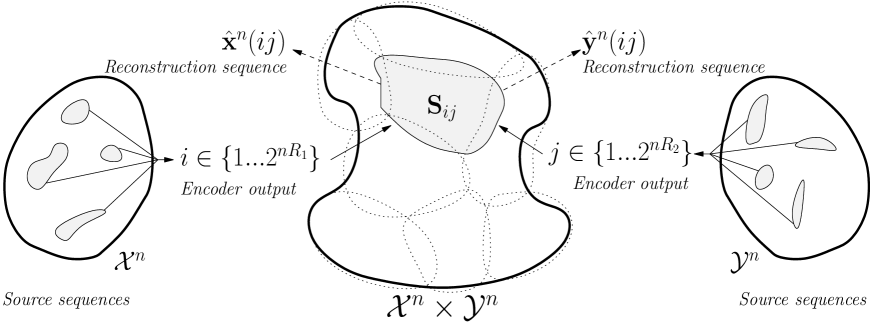
Figure 4: Cover-based representation of a distributed rate-distortion code.

I-C2 Constraints on the Structure of Source Covers

Our main insight is that, whereas in the classical problem any arbitrary cover defines a valid rate-distortion code, in multiterminal source coding this is no longer the case: covers of the product source $\mathcal{X}^{n}\times\mathcal{Y}^{n}$ only of the form $\mathbf{S}_{ij}=\mathbf{S}_{1,i}\times\mathbf{S}_{2,j}$ can be realized by distributed codes. The significance of this requirement is illustrated with an example in Fig. 5.

         

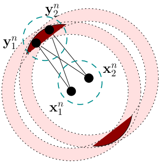
Figure 5: An example, to illustrate the significance of the requirement that cover elements $\mathbf{S}_{ij}$ take a product form. Let $\mathcal{X}=\mathcal{Y}=\{0,1\}$, and $p(xy)=p(x)p(y|x)$ specified by a $p(x)$ such that $P(X=0)=P(X=1)=\frac{1}{2}$, and $p(y|x)$ a binary symmetric channel with crossover probability $p_{c}$. Left: for each typical $\mathbf{x}^{n}$, there is a “ring” of $\mathbf{y}^{n}$’s jointly typical with it, centered at $\mathbf{x}^{n}$ and of radius $\approx np_{c}$. Right: consider pairs $\big{(}\mathbf{x}_{1}^{n}\mathbf{y}_{1}^{n}\big{)}$ and $\big{(}\mathbf{x}_{2}^{n}\mathbf{y}_{2}^{n}\big{)}$ in $\mathbf{S}_{ij}$; dashed circles denote distortion balls centered at $\hat{\mathbf{x}}^{n}(ij)$ and $\hat{\mathbf{y}}^{n}(ij)$ (with the centers omitted, for clarity), and dark shaded regions denote the intersection of two rings. Suppose now that all four pairs $(\mathbf{x}_{1}^{n}\mathbf{y}_{1}^{n})$, $(\mathbf{x}_{1}^{n}\mathbf{y}_{2}^{n})$ $(\mathbf{x}_{2}^{n}\mathbf{y}_{1}^{n})$, and $(\mathbf{x}_{2}^{n}\mathbf{y}_{2}^{n})$ are in $T_{\epsilon}^{n}\big{(}XY\big{)}$. Because $\mathbf{S}_{ij}=\mathbf{S}_{1,i}\times\mathbf{S}_{2,j}$, all four pairs must be in $\mathbf{S}_{ij}$ as well: the decoder does not have enough information to discriminate among these pairs. No such constraint exists with a centralized encoder.

From the informal argument of Fig. 5, we see how the fact that distributed codes produce covers only of the form $\mathbf{S}_{ij}=\mathbf{S}_{1,i}\times\mathbf{S}_{2,j}$ results in constraints on the sets used to cover the typical set $T_{\epsilon}^{n}\big{(}XY\big{)}$: there are certain groups of typical sequences that cannot be broken, in the sense that either all of them appear together in a cover element $\mathbf{S}_{ij}$, or none of them appear. We believe this is significant for two main reasons:

• If we compare to a classical rate-distortion code, this constraint is clearly not there. Provided the distortion constraints are met, a classical code would be able to split the typical set into distortion balls, without any further constraints.

• More fundamentally though, we view this constraint as a form of “independence,” reminiscent to us of the extra independence assumption required by the long Markov chain used in the definition of the Berger-Tung inner bound, which is not there in the definition of the outer bound, as highlighted in Section I-B earlier.

This latter observation is perhaps the strongest piece of evidence that suggested to us that the Berger-Tung inner bound might be tight.

I-D Main Contributions and Organization of the Paper

The main contribution presented in Part I of this paper is the development of an outer bound to the region of achievable rates for multiterminal source coding. This outer bound has two salient properties that distinguish it from existing bounds in the literature:

• it is based on explicitly modeling a constraint on the structure of codes that, as we understand things, had not been captured by any previously developed bound;

• and also unlike existing bounds, it is finitely parameterized.

We believe that this outer bound coincides with the set of achievable rates defined by the Berger-Tung inner bound. This issue is thoroughly explored in Part II of this paper, in the context of our study of algorithmic issues involved in the effective computation of this bound.

The rest of this paper is organized as follows. In Section II we define our notation, and state our main result. In Section III we state and prove some auxiliary lemmas that greatly simplify the proof of the main theorem, a proof that is fully developed in Section IV. The paper concludes with an extensive discussion on our main result and its implications, in Section V.

II Preliminaries

II-A Definitions and Notation

First, a word about notation. Random variables are denoted with capital letters, e.g., $X$. Realizations of these variables are denoted with lower case letters: e.g., $X=x$ means that the random variable $X$ takes on the value $x$. Script letters are typically used to denote alphabets, e.g., the random variable $X$ takes values on an alphabet $\mathcal{X}$. The alphabets of all random variables considered in this work are always assumed finite. Sets in general are denoted by capital boldface symbols, e.g., $\mathbf{S}$. The size of a set is denoted by $\big{|}\mathbf{S}\big{|}$. A probability mass function on $\mathcal{X}$ is denoted by $p_{X}(x)$, or simply $p(x)$ when the variable that it applies to is clear from the context. Sequences of elements from an alphabet $\mathcal{X}$ are denoted by boldface symbols $\mathbf{x}^{n}$, and its $i$-th element by $\mathbf{x}_{i}$; this sequence is an element of the extension alphabet $\mathcal{X}^{n}$. The expression $\mathbf{x}_{i}^{j,n}$ denotes a subsequence of $\mathbf{x}^{n}$ consisting of the elements $[\mathbf{x}_{i},\mathbf{x}_{i+1},...,\mathbf{x}_{j}]$, whenever $i\leq j$, otherwise it denotes an empty sequence; also, sometimes the length $n$ of the sequence will be clear from the context, and then we simply write $\mathbf{x}_{i}^{j}$ instead of $\mathbf{x}_{i}^{j,n}$, whenever this does not cause confusion. The expression $\mathbf{x}^{-i,n}$ denotes the sequence $[\mathbf{x}_{1},...,\mathbf{x}_{i-1},\mathbf{x}_{i+1},...,\mathbf{x}_{n}]$, and again, we write this as $\mathbf{x}^{-i}$ whenever $n$ is clear from the context. The same conventions are followed for sequences of random variables.

Given a boolean predicate $b(\mathbf{x})$ depending on a variable $\mathbf{x}$, we write $1_{\{b(\mathbf{x})\}}$ to denote the indicator function for the predicate: this is a function that takes the value 1 whenever $b(\mathbf{x})$ is true, and 0 whenever it is false. Given a sequence $\mathbf{x}^{n}\in\mathcal{X}^{n}$, and an element $x\in\mathcal{X}$, we denote by $N(x;\mathbf{x}^{n})$ the type of $\mathbf{x}^{n}$, defined as $N(x;\mathbf{x}^{n})=\sum_{i=1}^{n}1_{\{\mathbf{x}_{i}=x\}}$. Then, for any random variable $X$, any real number $\epsilon>0$, and any integer $n>0$, we denote by $T_{\epsilon}^{n}(X)$ the strongly typical set of $X$ with parameters $n$ and $\epsilon$, defined as

$$T_{\epsilon}^{n}(X)\;\;=\;\;\Big{\{}\mathbf{x}^{n}\in\mathcal{X}^{n}\;\Big{|}\;\forall x\in\mathcal{X}:\big{|}\mbox{$\frac{1}{n}$}N(x;\mathbf{x}^{n})-p_{X}(x)\big{|}<\mbox{$\frac{\epsilon}{|\mathcal{X}|}$}\Big{\}}.$$

In some situations, we need to compare typical sets defined for the same set of variables, but induced by different distributions on these variables. To resolve this ambiguity, we denote by $T_{\epsilon}^{n}\big{(}X\big{)}[p_{X}]$ the typical set corresponding to a distribution $p_{X}$. The same convention is followed when there is similar ambiguity in the evaluation of entropies (denoted $H\big{(}X\big{)}[p_{X}]$), and mutual information expressions (denoted $I\big{(}X\wedge Y\big{)}[p_{XY}]$).

Vector extensions $N(xy;\mathbf{x}^{n}\mathbf{y}^{n})$, $T_{\epsilon}^{n}(XY)$, etc., are defined by considering the same definitions as above, over a suitable product alphablet $\mathcal{X}\times\mathcal{Y}$. Similarly, given two random variables $X$ and $Y$, a joint probability mass function $p_{XY}(xy)$, and a sequence $\mathbf{y}^{n}$, we denote by $T_{\epsilon}^{n}(X|\mathbf{y}^{n})$ the conditional typical set of $X$ given $\mathbf{y}^{n}$, defined as

$$T_{\epsilon}^{n}\big{(}X\big{|}\mathbf{y}^{n}\big{)}\;\;=\;\;\Big{\{}\mathbf{x}^{n}\in\mathcal{X}^{n}\;\Big{|}\;\forall x\in\mathcal{X},y\in\mathcal{Y}:\big{|}\mbox{$\frac{1}{n}$}N(xy;\mathbf{x}^{n}\mathbf{y}^{n})-p_{XY}(xy)\big{|}<\mbox{$\frac{\epsilon}{|\mathcal{X}||\mathcal{Y}|}$}\Big{\}}.$$

We will also consider situations where we need to refer to the set of all typical sequences which are jointly typical with at least one of a group. In that case, for a set $\mathbf{S}\subseteq\mathcal{Y}^{n}$, we write

$$T_{\epsilon}^{n}\big{(}X\big{|}\mathbf{S}\big{)}\;\;=\;\;\bigcup_{\mathbf{y}^{n}\in\mathbf{S}}T_{\epsilon}^{n}\big{(}X\big{|}\mathbf{y}^{n}\big{)}.$$

Given any $\epsilon>0$, many times we require to make reference to quantities which are deterministic functions of $\epsilon$, having the property that as $\epsilon\to 0$, these quantities also vanish. Such small quantities are denoted by $\epsilon_{1}$, $\epsilon_{2}$, $\dot{\epsilon}$, $\ddot{\epsilon}$, $\epsilon^{\prime}$, $\epsilon^{\prime\prime}$, etc.; and the value of $\epsilon$ on which they depend is either mentioned explicitly or should be clear from the context.

Consider two random variables $X$ and $Y$ with joint distribution $p(xy)$. $T_{\epsilon}^{n}\big{(}X)$ is the usual typical set. Sometimes we also need to consider the set $S_{\epsilon,Y}^{n}(X)\triangleq\Big{\{}\mathbf{x}^{n}\,\Big{|}\,T_{\epsilon}^{n}\big{(}Y\big{|}\mathbf{x}^{n}\big{)}\neq\emptyset\Big{\}}$. Clearly, $S_{\epsilon,Y}^{n}(X)\subseteq T_{\epsilon}^{n}\big{(}X)$. But we also know from [25, Ch. 5], that $\Big{|}\frac{1}{n}\log\big{|}S_{\epsilon,Y}^{n}(X)\big{|}-H(X)\Big{|}<\dot{\epsilon}$. That is, although there may exist strongly typical sequences $\mathbf{x}^{n}$ for which there are no sequences $\mathbf{y}^{n}$ jointly typical with them, these $\mathbf{x}^{n}$’s form a set of vanishing measure.

Some standard operations on sets are intersection ($\mathbf{A}\cap\mathbf{B}$), union ($\mathbf{A}\cup\mathbf{B}$), complementation ($\mathbf{A}^{c}$) and difference ($\mathbf{A}\backslash\mathbf{B}$). The set of all subsets of $\mathbf{S}$ is denoted by $2^{\mathbf{S}}$. The convex closure of $\mathbf{S}$ is denoted by $\overline{\mathbf{S}}=\bigcap\big{\{}\mathbf{S}^{\prime}\;\big{|}\;\mathbf{S}\subseteq\mathbf{S}^{\prime}\,\wedge\,\mathbf{S}^{\prime}\mbox{ is closed and convex}\big{\}}$. Given a set $\mathbf{S}$, a cover of size $N$ of $\mathbf{S}$ is a collection of sets $\mathcal{S}=\big{\{}\mathbf{S}_{i}:i=1...N\big{\}}$, such that $\mathbf{S}\subseteq\bigcup_{i=1}^{N}\mathbf{S}_{i}$. If a cover further satisfies that $\mathbf{S}_{i}\cap\mathbf{S}_{j}=\emptyset$ ($1\leq i\neq j\leq N$), and that $\mathbf{S}=\bigcup_{i=1}^{N}\mathbf{S}_{i}$, then we say that $\mathcal{S}$ is a partition of $\mathbf{S}$.

Consider two sets, $\mathbf{A}$ and $\mathbf{B}$, for which $P\big{(}\mathbf{B}\big{|}\mathbf{A}\big{)}=1$: clearly, $P\big{(}\mathbf{A}\cap\mathbf{B}\big{)}=P\big{(}\mathbf{A}\big{)}$, and hence $\mathbf{A}\subseteq\mathbf{B}$, except perhaps for a set of measure zero. If instead we have a slightly weaker condition, namely that $P\big{(}\mathbf{B}\big{|}\mathbf{A}\big{)}>1-\epsilon$, then we say that $\mathbf{A}$ is weakly included in $\mathbf{B}$, and we denote this by $\mathbf{A}\subseteq_{\epsilon}\mathbf{B}$.

II-B Distributed Rate-Distortion Codes

Consider two sources $X$ and $Y$, out of which random pairs of sequences $\big{(}X^{n},Y^{n}\big{)}$ are drawn i.i.d. $\sim p(xy)$ from two finite alphabets, denoted $\mathcal{X}$ and $\mathcal{Y}$, and reproduced with elements of two other alphabets $\hat{\mathcal{X}}$ and $\hat{\mathcal{Y}}$. The two sources $X$ and $Y$ are processed by two separate encoders. The encoders are two functions:

$$f_{1}:\;\mathcal{X}^{n}\;\;\to\;\;\big{\{}1,2,\dots,2^{nR_{1}}\big{\}}\mbox{\hskip 28.45274ptand\hskip 28.45274pt}f_{2}:\;\mathcal{Y}^{n}\;\;\to\;\;\big{\{}1,2,\dots,2^{nR_{2}}\big{\}}.$$

These encoding functions map a block of $n$ source symbols to discrete indices. The decoder is a function

$$g:\;\big{\{}1,2,\dots,2^{nR_{1}}\big{\}}\times\big{\{}1,2,\dots,2^{nR_{2}}\big{\}}\;\;\to\;\;\hat{\mathcal{X}}^{n}\times\hat{\mathcal{Y}}^{n},$$

which maps a pair of indices into two blocks of reconstructed source sequences.

Two distortion measures $d_{1}:\mathcal{X}\times\hat{\mathcal{X}}\to[0,\infty)$ and $d_{2}:\mathcal{Y}\times\hat{\mathcal{Y}}\to[0,\infty)$ are used to define reconstruction quality. Since $\infty$ is not in their range and the alphabets are finite, these distortion measures are necessarily bounded, so we denote these largest values by $\max\limits_{x\in\mathcal{X},\hat{x}\in\hat{\mathcal{X}}}d_{1}(x,\hat{x})\triangleq d_{1,\mbox{\tiny MAX}}$, $\max\limits_{y\in\mathcal{Y},\hat{y}\in\hat{\mathcal{Y}}}d_{2}(y,\hat{y})\triangleq d_{2,\mbox{\tiny MAX}}$, and $\max\big{(}d_{1,\mbox{\tiny MAX}},d_{2,\mbox{\tiny MAX}}\big{)}\triangleq d_{\mbox{\tiny MAX}}<\infty$. $d_{1}^{n}\big{(}\mathbf{x}^{n},\hat{\mathbf{x}}^{n}\big{)}\triangleq\frac{1}{n}\sum_{i=1}^{n}d_{1}\big{(}x_{i},\hat{x}_{i}\big{)}$ and $d_{2}^{n}\big{(}\mathbf{y}^{n},\hat{\mathbf{y}}^{n}\big{)}\triangleq\frac{1}{n}\sum_{i=1}^{n}d_{2}\big{(}y_{i},\hat{y}_{i}\big{)}$ denote the corresponding extensions to blocks. Oftentimes, the symbols $d_{1}$ and $d_{2}$ are used for both the single-letter and the block extensions; which is the intended meaning should be clear from the context. For any distortion measure $d:\mathcal{X}^{n}\times\hat{\mathcal{X}}^{n}\to[0,\infty)$, an element $\hat{\mathbf{x}}^{n}\in\hat{\mathcal{X}}^{n}$ and a number $D\geq 0$, a “ball” of radius $D$ centered at $\hat{\mathbf{x}}^{n}$ is the set $B\big{(}\hat{\mathbf{x}}^{n},D\big{)}=\big{\{}\mathbf{x}^{n}\in\mathcal{X}^{n}\,\big{|}\,d\big{(}\mathbf{x}^{n},\hat{\mathbf{x}}^{n}\big{)})<D\big{\}}$ (and similarly for a ball $B\big{(}\hat{\mathbf{y}}^{n},D\big{)}$). For any $D$, $D^{+}$ is shorthand for $D+\dot{\epsilon}$, for an $\epsilon$ that is always clear from the context.

Fix now encoders and decoder $(f_{1},f_{2},g)$ operating on blocks of length $n$, and a real number $\epsilon>0$. If we have that

$$P\Big{(}\Big{\{}\big{(}\mathbf{x}^{n}\mathbf{y}^{n}\big{)}\;\Big{|}\;\big{(}\hat{\mathbf{x}}^{n}\hat{\mathbf{y}}^{n}\big{)}=g\big{(}f_{1}(\mathbf{x}^{n}),f_{2}(\mathbf{y}^{n})\big{)}\,\wedge\,d_{1}\big{(}\mathbf{x}^{n},\hat{\mathbf{x}}^{n}\big{)}<D_{1}^{+}\,\wedge\,d_{2}\big{(}\mathbf{y}^{n},\hat{\mathbf{y}}^{n}\big{)}<D_{2}^{+}\Big{\}}\Big{)}\;\;\geq\;\;1-\dot{\epsilon},$$ (1)

then we say that $(f_{1},f_{2},g)$ satisfies the $(\epsilon,D_{1},D_{2})$-distortion constraint.

II-C Achievable Rates

A $\big{(}2^{nR_{1}},2^{nR_{2}},n,\epsilon,D_{1},D_{2}\big{)}$ distributed rate-distortion code is defined by a block length $n$, a parameter $\epsilon>0$, two encoding functions $f_{1}$ and $f_{2}$ with ranges of size $2^{nR_{1}}$ and $2^{nR_{2}}$, and a decoding function $g$, such that $(f_{1},f_{2},g)$ satisfies the $\big{(}\epsilon,D_{1},D_{2}\big{)}$-distortion constraints.

We say that the rate-distortion tuple $(R_{1},R_{2},D_{1},D_{2})$ is $\epsilon$-achievable if a $\big{(}2^{nR_{1}},2^{nR_{2}},n,\epsilon,D_{1},D_{2}\big{)}$ distributed code exists; for fixed parameters $\big{(}\epsilon,D_{1},D_{2}\big{)}$, we denote the set of all $\epsilon$-achievable pairs $(R_{1},R_{2})$ by $\mathcal{R}_{\epsilon}(D_{1},D_{2})$. Then, the rate region ${\cal R}^{*}(D_{1},D_{2})$ of the two sources is defined by

$$\mathcal{R}^{*}(D_{1},D_{2})\;\;\triangleq\;\;\bigcap_{\epsilon>0}\,\mathcal{R}_{\epsilon}(D_{1},D_{2}).$$

Now we are going to describe a different set of rates. Define $\mathbb{P}_{\mbox{\tiny LB}}$ to be the set of all probability distributions $p(xy\hat{x}\hat{y})$ over $\mathcal{X}\times\mathcal{Y}\times\hat{\mathcal{X}}\times\hat{\mathcal{Y}}$, such that:

• $p(xy\hat{x}\hat{y})=p(\hat{x}\hat{y})p(x|\hat{x}\hat{y})p(y|\hat{x}\hat{y})$ (that is, $X-\hat{X}\hat{Y}-Y$ forms a Markov chain);

• $p_{XY}=\sum_{\hat{x}\hat{y}}p(\hat{x}\hat{y})p(x|\hat{x}\hat{y})p(y|\hat{x}\hat{y})$ ($p_{XY}$ is the source);

• and $\operatorname{E}\left[d_{1}\big{(}X,\hat{X}\big{)}\right]\leq D_{1}$ and $\operatorname{E}\left[d_{2}\big{(}Y,\hat{Y}\big{)}\right]\leq D_{2}$.

Then, for each $p\in\mathbb{P}_{\mbox{\tiny LB}}$, define

$$\mathcal{R}\big{(}D_{1},D_{2},p\big{)}\;\;\triangleq\;\;\left\{(R_{1},R_{2})\;\left|\;\begin{array}[]{rcl}R_{1}&\geq&I\big{(}X\wedge\hat{X}\hat{Y}\big{|}Y\big{)}[p]\\ R_{2}&\geq&I\big{(}Y\wedge\hat{X}\hat{Y}\big{|}X\big{)}[p]\\ R_{1}+R_{2}&\geq&I\big{(}XY\wedge\hat{X}\hat{Y}\big{)}[p]\end{array}\right.\right\},$$

and define also $\mathcal{R}^{o}(D_{1},D_{2})\triangleq\bigcup_{p\in\mathbb{P}_{\mbox{\tiny LB}}}\mathcal{R}\big{(}D_{1},D_{2},p\big{)}$. Now we are ready to state our outer bound.

II-D Statement of an Outer Bound

Theorem 1

$$\mathcal{R}^{*}\big{(}D_{1},D_{2}\big{)}\;\;\subseteq\;\;\overline{\mathcal{R}^{o}(D_{1},D_{2})}.$$ $\square$

The proof of this theorem is given in Section IV. Before that, and next in Section III, we develop a number of observations and auxliary results to be used in the main proof.

III Some Useful Observations and Auxiliary Results

III-A Distributed Rate-Distortion Codes as Constrained Source Covers

III-A1 Distributed Source Covers

An equivalent representation for a generic $(2^{nR_{1}},2^{nR_{2}},n,\epsilon,D_{1},D_{2})$ code is given as follows:

• Two covers: $\mathcal{S}_{1}=\big{\{}\mathbf{S}_{1,i}:i=1...2^{nR_{1}}\big{\}}$ of $\mathcal{X}^{n}$, and $\mathcal{S}_{2}=\big{\{}\mathbf{S}_{2,j}:j=1...2^{nR_{2}}\big{\}}$ of $\mathcal{Y}^{n}$. Any code with encoders $f_{1}$ and $f_{2}$ can be represented in terms of two such covers, by considering $f_{1}^{-1}(i)=\mathbf{S}_{1,i}$ and $f_{2}^{-1}(j)=\mathbf{S}_{2,j}$.
  (Note: these two covers define a cover $\mathcal{S}=\big{(}\mathcal{S}_{1},\mathcal{S}_{2}\big{)}$ of $\mathcal{X}^{n}\times\mathcal{Y}^{n}$, with elements $\mathbf{S}_{ij}\;=\;\mathbf{S}_{1,i}\times\mathbf{S}_{2,j}$, for $(i,j)\in\{1...2^{nR_{1}}\}\times\{1...2^{nR_{2}}\}$.)

• A pair of reconstruction sequences $\big{(}\hat{\mathbf{x}}^{n}(ij),\hat{\mathbf{y}}^{n}(ij)\big{)}=g(i,j)$ associated to each cover element $\mathbf{S}_{ij}$ of the product source, for all $(i,j)\in\{1...2^{nR_{1}}\}\times\{1...2^{nR_{2}}\}$.

In general, whenever we refer to a distributed rate-distortion code, we use interchangeably the earlier representation in terms of two encoders and one decoder, and this representation in terms of covers.

III-A2 Distributed Typical Sets

As highlighted in the Introduction, it turns out that covers $\mathbf{S}_{ij}$ of the product source $\mathcal{X}^{n}\times\mathcal{Y}^{n}$ are constrained beyond the requirements imposed by the fidelity criteria. That “extra” structure is described by Proposition 2.

Proposition 2

For any cover $\mathcal{S}$ of $\mathcal{X}^{n}\times\mathcal{Y}^{n}$ defined by some $(2^{nR_{1}},2^{nR_{2}},n,\epsilon,D_{1},D_{2})$ distributed rate-distortion code, and for any $(i,j)\in\{1...2^{nR_{1}}\}\times\{1...2^{nR_{2}}\}$, $\mathbf{x}^{n}\in\mathbf{S}_{1,i}$ and $\mathbf{y}^{n}\in\mathbf{S}_{2,j}$, then it must be the case that either $(\mathbf{x}^{n}\mathbf{y}^{n})\in\mathbf{S}_{ij}\cap T_{\epsilon}^{n}\big{(}XY\big{)}$ or $(\mathbf{x}^{n}\mathbf{y}^{n})\not\in T_{\epsilon}^{n}\big{(}XY\big{)}$. $\square$

Proof. This is rather straightforward. Take any $\mathbf{x}^{n}\in\mathbf{S}_{1,i}$ and $\mathbf{y}^{n}\in\mathbf{S}_{2,j}$. Then:

• by construction, $\big{(}\mathbf{x}^{n}\mathbf{y}^{n}\big{)}\in\mathbf{S}_{ij}$;

• either $\big{(}\mathbf{x}^{n}\mathbf{y}^{n}\big{)}\in T_{\epsilon}^{n}\big{(}XY\big{)}$ or $\big{(}\mathbf{x}^{n}\mathbf{y}^{n}\big{)}\not\in T_{\epsilon}^{n}\big{(}XY\big{)}$ – a tautology;

• if $\big{(}\mathbf{x}^{n}\mathbf{y}^{n}\big{)}\in T_{\epsilon}^{n}\big{(}XY\big{)}$, then $\big{(}\mathbf{x}^{n}\mathbf{y}^{n}\big{)}\in\mathbf{S}_{ij}\cap T_{\epsilon}^{n}\big{(}XY\big{)}$, and therefore the proposition is proved;

• and if instead, $\big{(}\mathbf{x}^{n}\mathbf{y}^{n}\big{)}\not\in T_{\epsilon}^{n}\big{(}XY\big{)}$, then the proposition is proved too. $\blacksquare$

Proposition 2 formally states the property of covers arising from distributed codes discussed informally in the Introduction (cf. Sec. I-C1): all combinations of an $\mathbf{x}^{n}$ sequence in $\mathbf{S}_{1,i}$ and a $\mathbf{y}^{n}$ sequence in $\mathbf{S}_{2,j}$, if they are jointly typical, must appear in $\mathbf{S}_{ij}\cap T_{\epsilon}^{n}\big{(}XY\big{)}$ – the decoder does not have enough information to discriminate among such pairs.

We now introduce a new definition. Consider any subset $\mathbf{S}\subseteq T_{\epsilon}^{n}\big{(}XY\big{)}$ for which, for any $(\mathbf{x}^{n},\mathbf{y}_{1}^{n})\in\mathbf{S}$ and $(\mathbf{x}_{1}^{n},\mathbf{y}^{n})\in\mathbf{S}$, we have that either $(\mathbf{x}^{n}\mathbf{y}^{n})\in\mathbf{S}$ or $(\mathbf{x}^{n}\mathbf{y}^{n})\not\in T_{\epsilon}^{n}\big{(}XY\big{)}$ – that is, the property of Prop. 2 holds for $\mathbf{S}$. In this case, we say that $\mathbf{S}$ is is a distributed typical set.

Clearly there are “interesting” distributed typical sets, the concept is not vacuous:

• all sets of the form $\mathbf{S}=\{(\mathbf{x}^{n}\mathbf{y}^{n})\}$, with $(\mathbf{x}^{n}\mathbf{y}^{n})\in T_{\epsilon}^{n}\big{(}XY\big{)}$, are distributed typical sets;

• for any $\mathbf{S}_{1}\subseteq\mathcal{X}^{n}$ and any $\mathbf{S}_{2}\subseteq\mathcal{Y}^{n}$, $\mathbf{S}\triangleq\big{[}\mathbf{S}_{1}\!\times\!\mathbf{S}_{2}\big{]}\cap T_{\epsilon}^{n}\big{(}XY\big{)}$ is a distributed typical set.

The last example provides a natural way of systematically constructing distributed typical sets.

III-A3 Source Covers Made of Distributed Typical Sets

We show next that in multiterminal source coding, the source must be covered with distributed typical sets in which each of the two components of the set gets specified by a different encoder.

Consider a length $n$ $\big{(}f_{1},f_{2},g\big{)}$ code, satisfying the $(\epsilon,D_{1},D_{2})$-distortion constraint of eqn. (1):

$$P\Big{(}\Big{\{}\big{(}\mathbf{x}^{n}\mathbf{y}^{n}\big{)}\;\Big{|}\;\big{(}\hat{\mathbf{x}}^{n}\hat{\mathbf{y}}^{n}\big{)}=g\big{(}f_{1}(\mathbf{x}^{n}),f_{2}(\mathbf{y}^{n})\big{)}\,\wedge\,d_{1}\big{(}\mathbf{x}^{n},\hat{\mathbf{x}}^{n}\big{)}<D_{1}^{+}\,\wedge\,d_{2}\big{(}\mathbf{y}^{n},\hat{\mathbf{y}}^{n}\big{)}<D_{2}^{+}\Big{\}}\Big{)}$$

$$\stackrel{{\scriptstyle(a)}}{{=}} P\Big{(}\Big{\{}\big{(}\mathbf{x}^{n}\mathbf{y}^{n}\big{)}\;\Big{|}\;\big{(}\hat{\mathbf{x}}^{n}\hat{\mathbf{y}}^{n}\big{)}=g\big{(}f_{1}(\mathbf{x}^{n}),f_{2}(\mathbf{y}^{n})\big{)}\,\wedge\,d_{1}\big{(}\mathbf{x}^{n},\hat{\mathbf{x}}^{n}\big{)}<D_{1}^{+}\,\wedge\,d_{2}\big{(}\mathbf{y}^{n},\hat{\mathbf{y}}^{n}\big{)}<D_{2}^{+}\Big{\}}\cap\bigcup_{(i,j)}\mathbf{S}_{ij}\Big{)}$$

$$= P\Big{(}\bigcup_{(i,j)}\Big{\{}\big{(}\mathbf{x}^{n}\mathbf{y}^{n}\big{)}\;\Big{|}\;\big{(}\hat{\mathbf{x}}^{n}\hat{\mathbf{y}}^{n}\big{)}=g\big{(}f_{1}(\mathbf{x}^{n}),f_{2}(\mathbf{y}^{n})\big{)}\,\wedge\,d_{1}\big{(}\mathbf{x}^{n},\hat{\mathbf{x}}^{n}\big{)}<D_{1}^{+}\,\wedge\,d_{2}\big{(}\mathbf{y}^{n},\hat{\mathbf{y}}^{n}\big{)}<D_{2}^{+}\Big{\}}\cap\mathbf{S}_{ij}\Big{)}$$

$$\stackrel{{\scriptstyle(b)}}{{=}} P\Big{(}\bigcup_{(i,j)}\Big{\{}\big{(}\mathbf{x}^{n}\mathbf{y}^{n}\big{)}\;\Big{|}\;d_{1}\big{(}\mathbf{x}^{n},\hat{\mathbf{x}}^{n}(ij)\big{)}<D_{1}^{+}\,\wedge\,\mathbf{x}^{n}\in\mathbf{S}_{1,i}\,\wedge\,d_{2}\big{(}\mathbf{y}^{n},\hat{\mathbf{y}}^{n}(ij)\big{)}<D_{2}^{+}\,\wedge\,\mathbf{y}_{2}^{n}\in\mathbf{S}_{2,j}\Big{\}}\Big{)}$$

$$= P\Big{(}\bigcup_{(i,j)}\big{[}\mathbf{S}_{1,i}\!\times\!\mathbf{S}_{2,j}\big{]}\cap\big{[}B\big{(}\hat{\mathbf{x}}^{n}(ij),D_{1}^{+}\big{)}\!\times\!B\big{(}\hat{\mathbf{y}}^{n}(ij),D_{2}^{+}\big{)}\big{]}\,\Big{)}$$

$$\stackrel{{\scriptstyle(c)}}{{\geq}} 1-\dot{\epsilon},$$

where (a) follows from $\big{\{}\big{(}\mathbf{x}^{n}\mathbf{y}^{n}\big{)}\,\Big{|}\,\big{(}\hat{\mathbf{x}}^{n}\hat{\mathbf{y}}^{n}\big{)}=g\big{(}f_{1}(\mathbf{x}^{n}),f_{2}(\mathbf{y}^{n})\big{)}\,\wedge\,d_{1}\big{(}\mathbf{x}^{n},\hat{\mathbf{x}}^{n}\big{)}<D_{1}^{+}\,\wedge\,d_{2}\big{(}\mathbf{y}^{n},\hat{\mathbf{y}}^{n}\big{)}<D_{2}^{+}\big{\}}\;\subseteq\;\mathcal{X}^{n}\times\mathcal{Y}^{n}\;\subseteq\;\bigcup_{(i,j)}\mathbf{S}_{ij}$; (b) follows from $\mathbf{S}_{ij}=\mathbf{S}_{1,i}\times\mathbf{S}_{2,j}$; and (c) follows from the fact that the code under consideration satisfies the distortion constraint of eqn. (1). We also know, from basic properties of typical sets, that

$$P\Big{(}T_{\epsilon}^{n}\big{(}XY\big{)}\Big{)}\;\;\geq\;\;1-\epsilon,$$

and so, if we define $\tilde{\mathbf{S}}_{ij}\triangleq\big{[}\mathbf{S}_{1,i}\times\mathbf{S}_{2,j}\big{]}\cap T_{\epsilon}^{n}\big{(}XY\big{)}$, we see that

$$P\Big{(}\bigcup_{(i,j)}\big{[}\mathbf{S}_{1,i}\!\times\!\mathbf{S}_{2,j}\big{]}\cap\big{[}B\big{(}\hat{\mathbf{x}}^{n}(ij),D_{1}^{+}\big{)}\!\times\!B\big{(}\hat{\mathbf{y}}^{n}(ij),D_{2}^{+}\big{)}\big{]}\cap T_{\epsilon}^{n}\big{(}XY\big{)}\,\Big{)}$$ (2)

$$= P\left(\bigcup_{(i,j)}\tilde{\mathbf{S}}_{ij}\cap\big{[}B\big{(}\hat{\mathbf{x}}^{n}(ij),D_{1}^{+}\big{)}\!\times\!B\big{(}\hat{\mathbf{y}}^{n}(ij),D_{2}^{+}\big{)}\big{]}\right)$$

$$\geq 1-\ddot{\epsilon};$$

that is, since $\tilde{\mathbf{S}}_{ij}$ is a distributed typical set, the source must be covered with the fraction of such sets contained in pairs of balls centered at the reconstruction sequences; furthermore, we note that each component of the distributed typical set must be specified completely by each encoder.

III-B The “Reverse” Markov Lemma

III-B1 The Standard Form

Lemma 1 is the Markov lemma as stated in [4, pg. 202], in our own notation.

Lemma 1 (Markov)

Consider a Markov chain of the form $X-Z-Y$. Then, for all $\epsilon>0$,

$$\lim_{n\to\infty}P\Big{(}\big{(}X^{n},\mathbf{y}^{n}\big{)}\in T_{\epsilon}^{n}\big{(}XY\big{)}\;\Big{|}\;\big{(}Z^{n},\mathbf{y}^{n}\big{)}\in T_{\epsilon}^{n}\big{(}ZY\big{)}\Big{)}\;\;=\;\;1,$$

for any sequence $\mathbf{y}^{n}\in\mathcal{Y}^{n}$. $\square$

The lemma says that for every $\mathbf{y}^{n}\in\mathcal{Y}^{n}$, if the random vector $\big{(}Z^{n},\mathbf{y}^{n}\big{)}\in T_{\epsilon}^{n}\big{(}ZY\big{)}$, then the random vector $\big{(}X^{n},\mathbf{y}^{n}\big{)}\in T_{\epsilon}^{n}\big{(}XY\big{)}$, with high probability. This is not true in general: if we have two pairs of sequences $\big{(}\mathbf{x}^{n}\mathbf{z}^{n}\big{)}\in T_{\epsilon}^{n}\big{(}XZ\big{)}$ and $\big{(}\mathbf{z}^{n}\mathbf{y}^{n}\big{)}\in T_{\epsilon}^{n}\big{(}ZY\big{)}$, it is not always the case that $\big{(}\mathbf{x}^{n}\mathbf{z}^{n}\mathbf{y}^{n}\big{)}\in T_{\epsilon}^{n}\big{(}XZY\big{)}$, and therefore that $\big{(}\mathbf{x}^{n}\mathbf{y}^{n}\big{)}\in T_{\epsilon}^{n}\big{(}XY\big{)}$; that is, joint typicality is not a transitive relation. However, if $X-Z-Y$ forms a Markov chain, and then only in a high probability sense, said transitivity property holds.

III-B2 A Converse Statement

We are interested in a converse form of the Markov lemma. Suppose we are given an arbitrary distribution $p(xyz)$, whose typical sets satisfy the constraints imposed by the Markov lemma: can we say that $p$ itself must be a Markov chain? It turns out the answer is almost yes – if some arbitrary distribution $p$ induces typical sets like those of a Markov chain, then there must exist a Markov chain $p^{\prime}$ within $L_{1}$ distance $2\epsilon$ of $p$. This statement is made precise in the following lemma.

Lemma 2 (Reverse Markov)

Fix $n$, $\epsilon>0$. Consider any distribution $p(xyz)$ for which, for some $\mathbf{z}^{n}$, $$T_{\epsilon}^{n}\big{(}X\big{|}\mathbf{z}^{n}\big{)}[p]\times T_{\epsilon}^{n}\big{(}Y\big{|}\mathbf{z}^{n}\big{)}[p]\;\;=\;\;T_{\epsilon}^{n}\big{(}XY\big{|}\mathbf{z}^{n}\big{)}[p].$$ Define a Markov chain $p^{\prime}(xyz)=p(z)p(x|z)p(y|z)$, with the components $p(z)$, $p(x|z)$ and $p(y|z)$ taken from the given $p(xyz)$. Then, $\big{|}\big{|}p-p^{\prime}\big{|}\big{|}_{1}\,<\,2\epsilon$. $\square$

Proof. Consider any $\mathbf{z}^{n}$ for which $T_{\epsilon}^{n}\big{(}XY\big{|}\mathbf{z}^{n}\big{)}[p]\neq\emptyset$. Since $p^{\prime}$ is a Markov chain, from the direct form of the Markov lemma we know that

$$T_{\epsilon}^{n}\big{(}X\big{|}\mathbf{z}^{n}\big{)}[p^{\prime}]\times T_{\epsilon}^{n}\big{(}Y\big{|}\mathbf{z}^{n}\big{)}[p^{\prime}]\;\;\subseteq_{\epsilon^{\prime}}\;\;T_{\epsilon}^{n}\big{(}XY\big{|}\mathbf{z}^{n}\big{)}[p^{\prime}];$$

and clearly, $\emptyset\neq T_{\epsilon}^{n}\big{(}XY\big{|}\mathbf{z}^{n}\big{)}[p]=T_{\epsilon}^{n}\big{(}X\big{|}\mathbf{z}^{n}\big{)}[p]\times T_{\epsilon}^{n}\big{(}Y\big{|}\mathbf{z}^{n}\big{)}[p]=T_{\epsilon}^{n}\big{(}X\big{|}\mathbf{z}^{n}\big{)}[p^{\prime}]\times T_{\epsilon}^{n}\big{(}Y\big{|}\mathbf{z}^{n}\big{)}[p^{\prime}]$, since we choose $p^{\prime}$ to coincide with $p$ on the corresponding marginals, and from our choice of $\mathbf{z}^{n}$. So, this last inclusion can be written as

$$T_{\epsilon}^{n}\big{(}X\big{|}\mathbf{z}^{n}\big{)}[p]\times T_{\epsilon}^{n}\big{(}Y\big{|}\mathbf{z}^{n}\big{)}[p]\;\;\subseteq_{\epsilon^{\prime}}\;\;T_{\epsilon}^{n}\big{(}XY\big{|}\mathbf{z}^{n}\big{)}[p^{\prime}],$$

and therefore we see that

$$\emptyset\;\;\neq\;\;T_{\epsilon}^{n}\big{(}X\big{|}\mathbf{z}^{n}\big{)}[p]\times T_{\epsilon}^{n}\big{(}Y\big{|}\mathbf{z}^{n}\big{)}[p]\;\;\subseteq_{\epsilon^{\prime}}\;\;T_{\epsilon}^{n}\big{(}XY\big{|}\mathbf{z}^{n}\big{)}[p]\cap T_{\epsilon}^{n}\big{(}XY\big{|}\mathbf{z}^{n}\big{)}[p^{\prime}];$$

thus, there must exist at least one triplet of sequences $\big{(}\mathbf{x}^{n}\mathbf{y}^{n}\mathbf{z}^{n}\big{)}$ that is jointly typical under both $p$ and $p^{\prime}$. So for these particular sequences, it follows from the definition of strong typicality that both

$$\forall xyz:\big{|}\mbox{$\frac{1}{n}$}N\big{(}xyz;\mathbf{x}^{n}\mathbf{y}^{n}\mathbf{z}^{n}\big{)}-p(xyz)\big{|}\,<\,\mbox{$\frac{\epsilon}{|\mathcal{X}||\mathcal{Y}||\mathcal{Z}|}$}\;\textrm{ and }\;\forall xyz:\big{|}\mbox{$\frac{1}{n}$}N\big{(}xyz;\mathbf{x}^{n}\mathbf{y}^{n}\mathbf{z}^{n}\big{)}-p^{\prime}(xyz)\big{|}\,<\,\mbox{$\frac{\epsilon}{|\mathcal{X}||\mathcal{Y}||\mathcal{Z}|}$},$$

and therefore the $L_{1}$ norm of $p-p^{\prime}$ can be written as

$$\big{|}\big{|}p^{\prime}-p\big{|}\big{|}_{1} = \sum_{xyz}\big{|}p(xyz)-p^{\prime}(xyz)\big{|}$$

$$= \sum_{xyz}\big{|}p(xyz)-\mbox{$\frac{1}{n}$}N\big{(}xyz;\mathbf{x}^{n}\mathbf{y}^{n}\mathbf{z}^{n}\big{)}+\mbox{$\frac{1}{n}$}N\big{(}xyz;\mathbf{x}^{n}\mathbf{y}^{n}\mathbf{z}^{n}\big{)}-p^{\prime}(xyz)\big{|}$$

$$\leq \sum_{xyz}\big{|}\mbox{$\frac{1}{n}$}N\big{(}xyz;\mathbf{x}^{n}\mathbf{y}^{n}\mathbf{z}^{n}\big{)}-p(xyz)\big{|}+\sum_{xyz}\big{|}\mbox{$\frac{1}{n}$}N\big{(}xyz;\mathbf{x}^{n}\mathbf{y}^{n}\mathbf{z}^{n}\big{)}-p^{\prime}(xyz)\big{|}$$

$$< 2\epsilon,$$

thus proving the lemma. $\blacksquare$

Our interest in this question stems from the fact that, from the requirement to cover a product source with distributed typical sets, we do get constraints on the shape of various typical sets. So we need to characterize what distributions can give rise to those sets, and this lemma plays an important role in that.

III-C Upper Bounds on the Size of Distributed Typical Cover Elements

Lemma 3

Consider any $\big{(}2^{nR_{1}},2^{nR_{2}},n,\epsilon,D_{1},D_{2}\big{)}$ distributed rate-distortion code, represented by a cover $\mathcal{S}$. Then, there exists a distribution $\pi\in\mathbb{P}_{\mbox{\tiny LB}}$ such that, for all $(i,j)\in\{1...2^{nR_{1}}\}\times\{1...2^{nR_{2}}\}$ and all $\epsilon>0$, $$\big{|}\mathbf{S}_{ij}\,\cap\,T_{\epsilon}^{n}\big{(}XY\big{)}\big{|}\;\;\leq\;\;2^{n(H(XY|\hat{X}\hat{Y})[\pi]+\ddot{\epsilon})},$$ provided $n$ is large enough. Furthermore, for all $\mathbf{y}^{n}\in\mathcal{Y}^{n}$, $$\big{|}\mathbf{S}_{1,i}\cap T_{\epsilon}^{n}\big{(}X\big{|}\mathbf{y}^{n}\big{)}\big{|}\;\;\leq\;\;2^{n(H(X|\hat{X}\hat{Y}Y)[\pi]+\ddot{\epsilon}^{\prime})},$$ and similarly for all $\mathbf{x}^{n}\in\mathcal{X}^{n}$, $$\big{|}\mathbf{S}_{2,j}\cap T_{\epsilon}^{n}\big{(}Y\big{|}\mathbf{x}^{n}\big{)}\big{|}\;\;\leq\;\;2^{n(H(Y|\hat{X}\hat{Y}X)[\pi]+\ddot{\epsilon}^{\prime\prime})},$$ also provided $n$ is large enough. $\square$

Proof. From the two-terminal rate-distortion theorem [14, Thm. 2.2.3], we know there exists a distribution $p(xy\hat{x}\hat{y})=p(xy)p(\hat{x}\hat{y}|xy)$, with $p(xy)$ the given source, $\operatorname{E}\left[d_{1}\big{(}X,\hat{X}\big{)}\right]\leq D_{1}$ and $\operatorname{E}\left[d_{2}\big{(}Y,\hat{Y}\big{)}\right]\leq D_{2}$, and sequences $\hat{\mathbf{x}}^{n}(ij)$ and $\hat{\mathbf{y}}^{n}(ij)$ such that, for all $(i,j)\in\{1...2^{nR_{1}}\}\times\{1...2^{nR_{2}}\}$ and all $\epsilon>0$,

$$\tilde{\mathbf{S}}_{ij}\;\;\subseteq\;\;T_{\epsilon}^{n}\big{(}XY\big{|}\hat{\mathbf{x}}^{n}(ij)\hat{\mathbf{y}}^{n}(ij)\big{)},$$ (3)

provided $n$ is large enough. But since for distributed codes we have $\tilde{\mathbf{S}}_{ij}=\big{[}\mathbf{S}_{1,i}\times\mathbf{S}_{2,j}\big{]}\cap T_{\epsilon}^{n}\big{(}XY\big{)}$, it follows from standard properties of typical sets that

$$\mathbf{S}_{1,i}\cap T_{\epsilon}^{n}\big{(}X\big{|}\mathbf{S}_{2,j}\big{)}\;\;\subseteq\;\;T_{\epsilon}^{n}\big{(}X\big{|}\hat{\mathbf{x}}^{n}(ij)\hat{\mathbf{y}}^{n}(ij)\big{)}\mbox{\hskip 28.45274ptand\hskip 28.45274pt}\mathbf{S}_{2,j}\cap T_{\epsilon}^{n}\big{(}Y\big{|}\mathbf{S}_{1,i}\big{)}\;\;\subseteq\;\;T_{\epsilon}^{n}\big{(}Y\big{|}\hat{\mathbf{x}}^{n}(ij)\hat{\mathbf{y}}^{n}(ij)\big{)}.$$

Consider now a new cover $\mathcal{S}^{\prime}$, having the property that

$$\mathbf{S}^{\prime}_{1,i}\cap T_{\epsilon}^{n}\big{(}X\big{|}\mathbf{S}^{\prime}_{2,j}\big{)}\;\;=\;\;T_{\epsilon}^{n}\big{(}X\big{|}\hat{\mathbf{x}}^{n}(ij)\hat{\mathbf{y}}^{n}(ij)\big{)}\mbox{\hskip 28.45274ptand\hskip 28.45274pt}\mathbf{S}^{\prime}_{2,j}\cap T_{\epsilon}^{n}\big{(}X\big{|}\mathbf{S}^{\prime}_{1,i}\big{)}\;\;=\;\;T_{\epsilon}^{n}\big{(}Y\big{|}\hat{\mathbf{x}}^{n}(ij)\hat{\mathbf{y}}^{n}(ij)\big{)}.$$

A simple expression for the cover element $\mathbf{S}^{\prime}_{1,i}$ is obtained as follows. Fix an index $i\in\{1...2^{nR_{1}}\}$:

$$\begin{array}[]{lrcl}&\forall k:\mathbf{S}^{\prime}_{1,i}\cap T_{\epsilon}^{n}\big{(}X\big{|}\mathbf{S}^{\prime}_{2,k}\big{)}&=&T_{\epsilon}^{n}\big{(}X\big{|}\hat{\mathbf{x}}^{n}(ik)\hat{\mathbf{y}}^{n}(ik)\big{)}\\ \Rightarrow&\bigcup_{k=1}^{2^{nR_{2}}}\mathbf{S}^{\prime}_{1,i}\cap T_{\epsilon}^{n}\big{(}X\big{|}\mathbf{S}^{\prime}_{2,k}\big{)}&=&\bigcup_{k=1}^{2^{nR_{2}}}T_{\epsilon}^{n}\big{(}X\big{|}\hat{\mathbf{x}}^{n}(ik)\hat{\mathbf{y}}^{n}(ik)\big{)}\\ \Rightarrow&\mathbf{S}^{\prime}_{1,i}\cap\bigcup_{k=1}^{2^{nR_{2}}}T_{\epsilon}^{n}\big{(}X\big{|}\mathbf{S}^{\prime}_{2,k}\big{)}&=&\bigcup_{k=1}^{2^{nR_{2}}}T_{\epsilon}^{n}\big{(}X\big{|}\hat{\mathbf{x}}^{n}(ik)\hat{\mathbf{y}}^{n}(ik)\big{)}\\ \Rightarrow&\mathbf{S}^{\prime}_{1,i}\cap S_{\epsilon,Y}^{n}\big{(}X\big{)}&=&\bigcup_{k=1}^{2^{nR_{2}}}T_{\epsilon}^{n}\big{(}X\big{|}\hat{\mathbf{x}}^{n}(ik)\hat{\mathbf{y}}^{n}(ik)\big{)},\end{array}$$

and since $P\big{(}S_{\epsilon,Y}^{n}\big{(}X\big{)}\big{)}>1-\dot{\epsilon}$, $\mathbf{S}^{\prime}_{1,i}$ is determined up to a set of vanishing measure; similarly, fixing $j\in\{1...2^{nR_{2}}\}$, we get $\mathbf{S}^{\prime}_{2,j}\cap S_{\epsilon,X}^{n}\big{(}Y\big{)}=\bigcup_{l=1}^{2^{nR_{1}}}T_{\epsilon}^{n}\big{(}Y\big{|}\hat{\mathbf{x}}^{n}(lj)\hat{\mathbf{y}}^{n}(lj)\big{)}$.

The new cover $\mathcal{S}^{\prime}$ has some useful properties:

• for all $(i,j)$, $\mathbf{S}_{1,i}\cap S_{\epsilon,Y}^{n}\big{(}X\big{)}\subseteq\mathbf{S}^{\prime}_{1,i}\cap S_{\epsilon,Y}^{n}\big{(}X\big{)}$ and $\mathbf{S}_{2,j}\cap S_{\epsilon,X}^{n}\big{(}Y\big{)}\subseteq\mathbf{S}^{\prime}_{2,j}\cap S_{\epsilon,X}^{n}\big{(}Y\big{)}$, and therefore $\tilde{\mathbf{S}}_{ij}\subseteq\tilde{\mathbf{S}}^{\prime}_{ij}$ as well, by construction;

• for all $\big{(}\mathbf{x}^{n}\mathbf{y}^{n}\big{)}\in\tilde{\mathbf{S}}^{\prime}_{ij}$, $d_{1}\big{(}\mathbf{x}^{n},\hat{\mathbf{x}}^{n}(ij)\big{)}<D_{1}^{+}$ and $d_{2}\big{(}\mathbf{y}^{n},\hat{\mathbf{y}}^{n}(ij)\big{)}<D_{2}^{+}$, from the joint typicality conditions defining $\mathbf{S}^{\prime}_{1,i}$ and $\mathbf{S}^{\prime}_{2,j}$;

• and $P\Big{(}\bigcup_{ij}\tilde{\mathbf{S}}^{\prime}_{ij}\Big{)}\geq P\Big{(}\bigcup_{ij}\tilde{\mathbf{S}}_{ij}\Big{)}>1-\dot{\epsilon}$;

so, $\mathcal{S}^{\prime}$ “dominates” $\mathcal{S}$ (in that every element in $\mathcal{S}$ is contained in one element of $\mathcal{S}^{\prime}$), and $\mathcal{S}^{\prime}$ satisfies the same distortion constraints that $\mathcal{S}$ does. Therefore, an upper bound on the size of the elements in the new cover $\mathcal{S}^{\prime}$ is also an upper bound on the size of the elements in the given cover $\mathcal{S}$.

Next we observe that new cover element $\tilde{\mathbf{S}}^{\prime}_{ij}$ can be “sandwiched” in between two other terms:

$$\Big{[}T_{\epsilon}^{n}\big{(}X\big{|}\hat{\mathbf{x}}^{n}(ij)\hat{\mathbf{y}}^{n}(ij)\big{)}\times T_{\epsilon}^{n}\big{(}Y\big{|}\hat{\mathbf{x}}^{n}(ij)\hat{\mathbf{y}}^{n}(ij)\big{)}\Big{]}\cap T_{\epsilon}^{n}\big{(}XY\big{)} \stackrel{{\scriptstyle(a)}}{{\subseteq}} \big{[}\mathbf{S}^{\prime}_{1,i}\times\mathbf{S}^{\prime}_{2,j}\big{]}\cap T_{\epsilon}^{n}\big{(}XY\big{)}$$

$$\stackrel{{\scriptstyle(b)}}{{\subseteq}} T_{\epsilon}^{n}\big{(}XY\big{|}\hat{\mathbf{x}}^{n}(ij)\hat{\mathbf{y}}^{n}(ij)\big{)},$$

where (a) follows from our choice of $\mathbf{S}^{\prime}_{1,i}$ and $\mathbf{S}^{\prime}_{2,j}$, and from elementary algebra of sets; and (b) follows from eqn. (3), and from the product form of distributed covers. So, since the other inclusion always holds,

$$\Big{[}T_{\epsilon}^{n}\big{(}X\big{|}\hat{\mathbf{x}}^{n}(ij)\hat{\mathbf{y}}^{n}(ij)\big{)}\times T_{\epsilon}^{n}\big{(}Y\big{|}\hat{\mathbf{x}}^{n}(ij)\hat{\mathbf{y}}^{n}(ij)\big{)}\Big{]}\cap T_{\epsilon}^{n}\big{(}XY\big{)}\;\;=\;\;T_{\epsilon}^{n}\big{(}XY\big{|}\hat{\mathbf{x}}^{n}(ij)\hat{\mathbf{y}}^{n}(ij)\big{)}$$

is a necessary condition on any suitable distribution $p(xy\hat{x}\hat{y})$ whose typical sets can be used to construct the cover $\mathcal{S}^{\prime}$; or equivalently, since this must hold for every $(i,j)$,

$$\Big{[}T_{\epsilon}^{n}\big{(}X\big{|}\hat{\mathbf{x}}^{n}\hat{\mathbf{y}}^{n}\big{)}\times T_{\epsilon}^{n}\big{(}Y\big{|}\hat{\mathbf{x}}^{n}\hat{\mathbf{y}}^{n}\big{)}\Big{]}\cap T_{\epsilon}^{n}\big{(}XY\big{)}\;\;=\;\;T_{\epsilon}^{n}\big{(}XY\big{|}\hat{\mathbf{x}}^{n}\hat{\mathbf{y}}^{n}\big{)},$$

for any sequences $\hat{\mathbf{x}}^{n}$ and $\hat{\mathbf{y}}^{n}$ such that $T_{\epsilon}^{n}\big{(}XY\big{|}\hat{\mathbf{x}}^{n}\hat{\mathbf{y}}^{n}\big{)}\neq\emptyset$. Finally we note that this last condition is equivalent to

$$T_{\epsilon}^{n}\big{(}X\big{|}\hat{\mathbf{x}}^{n}\hat{\mathbf{y}}^{n}\big{)}\times T_{\epsilon}^{n}\big{(}Y\big{|}\hat{\mathbf{x}}^{n}\hat{\mathbf{y}}^{n}\big{)}\;\;=\;\;T_{\epsilon}^{n}\big{(}XY\big{|}\hat{\mathbf{x}}^{n}\hat{\mathbf{y}}^{n}\big{)}.$$ (4)

This is because this last equality already forces any $\mathbf{x}^{n}\in T_{\epsilon}^{n}\big{(}X\big{|}\hat{\mathbf{x}}^{n}\hat{\mathbf{y}}^{n}\big{)}$ and $\mathbf{y}^{n}\in T_{\epsilon}^{n}\big{(}Y\big{|}\hat{\mathbf{x}}^{n}\hat{\mathbf{y}}^{n}\big{)}$ to be jointly typical. Therefore, from the reverse Markov lemma, we conclude there exists a distribution $\pi(xy\hat{x}\hat{y})$, which satisfies a Markov chain of the form $X-\hat{X}\hat{Y}-Y$, such that $\big{|}\big{|}p-\pi\big{|}\big{|}_{1}<2\epsilon$.

———————

Next we observe that if $\big{|}\big{|}p-\pi\big{|}\big{|}_{1}<2\epsilon$, then conditionals and marginals of $p$ and of $\pi$ are also close. Consider, for example, $p_{\hat{X}\hat{Y}}(\hat{x}\hat{y})=\sum_{xy}p_{XY\hat{X}\hat{Y}}(xy\hat{x}\hat{y})$ and $\pi_{\hat{X}\hat{Y}}(\hat{x}\hat{y})=\sum_{xy}\pi_{XY\hat{X}\hat{Y}}(xy\hat{x}\hat{y})$:

$$\big{|}\big{|}p_{\hat{X}\hat{Y}}(\cdot)-\pi_{\hat{X}\hat{Y}}(\cdot)\big{|}\big{|}_{1} = \sum_{\hat{x}\hat{y}}\big{|}p_{\hat{X}\hat{Y}}(\hat{x}\hat{y})-\pi_{\hat{X}\hat{Y}}(\hat{x}\hat{y})\big{|}$$

$$= \sum_{\hat{x}\hat{y}}\Big{|}\Big{(}\sum_{x^{\prime}y^{\prime}}p_{XY\hat{X}\hat{Y}}(x^{\prime}y^{\prime}\hat{x}\hat{y})\Big{)}-\Big{(}\sum_{x^{\prime\prime}y^{\prime\prime}}\pi_{XY\hat{X}\hat{Y}}(x^{\prime\prime}y^{\prime\prime}\hat{x}\hat{y})\Big{)}\Big{|}$$

$$= \sum_{\hat{x}\hat{y}}\Big{|}\sum_{xy}p_{XY\hat{X}\hat{Y}}(xy\hat{x}\hat{y})-\pi_{XY\hat{X}\hat{Y}}(xy\hat{x}\hat{y})\Big{|}$$

$$\leq \sum_{xy\hat{x}\hat{y}}\big{|}p_{XY\hat{X}\hat{Y}}(xy\hat{x}\hat{y})-\pi_{XY\hat{X}\hat{Y}}(xy\hat{x}\hat{y})\big{|}$$

$$< 2\epsilon.$$

For the conditional $p_{XY|\hat{X}\hat{Y}}(xy|\hat{x}\hat{y})$:

$$\big{|}\big{|}p_{XY|\hat{X}\hat{Y}}(\cdot|\hat{x}\hat{y})-\pi_{XY|\hat{X}\hat{Y}}(\cdot|\hat{x}\hat{y})\big{|}\big{|}_{1}\;\;=\;\;\sum_{xy}\big{|}p_{XY|\hat{X}\hat{Y}}(xy|\hat{x}\hat{y})-p_{XY|\hat{X}\hat{Y}}(xy|\hat{x}\hat{y})\big{|}$$

$$= \sum_{xy}\Big{|}\frac{p_{XY\hat{X}\hat{Y}}(xy\hat{x}\hat{y})}{p_{\hat{X}\hat{Y}}(\hat{x}\hat{y})}-\frac{\pi_{XY\hat{X}\hat{Y}}(xy\hat{x}\hat{y})}{\pi_{\hat{X}\hat{Y}}(\hat{x}\hat{y})}\Big{|}$$

$$= \mbox{$\frac{1}{p_{\hat{X}\hat{Y}}(\hat{x}\hat{y})\pi_{\hat{X}\hat{Y}}(\hat{x}\hat{y})}$}\sum_{xy}\big{|}p_{XY\hat{X}\hat{Y}}(xy\hat{x}\hat{y})\pi_{\hat{X}\hat{Y}}(\hat{x}\hat{y})-\pi_{XY\hat{X}\hat{Y}}(xy\hat{x}\hat{y})p_{\hat{X}\hat{Y}}(\hat{x}\hat{y})\big{|}$$

$$\stackrel{{\scriptstyle(a)}}{{<}} \mbox{$\frac{1}{p_{\hat{X}\hat{Y}}(\hat{x}\hat{y})\pi_{\hat{X}\hat{Y}}(\hat{x}\hat{y})}$}\sum_{xy}\big{|}p_{XY\hat{X}\hat{Y}}(xy\hat{x}\hat{y})p_{\hat{X}\hat{Y}}(\hat{x}\hat{y})+p_{XY\hat{X}\hat{Y}}(xy\hat{x}\hat{y})2\epsilon-\pi_{XY\hat{X}\hat{Y}}(xy\hat{x}\hat{y})p_{\hat{X}\hat{Y}}(\hat{x}\hat{y})\big{|}$$

$$\leq \mbox{$\frac{1}{p_{\hat{X}\hat{Y}}(\hat{x}\hat{y})\pi_{\hat{X}\hat{Y}}(\hat{x}\hat{y})}$}\sum_{xy}\Big{(}2\epsilon p_{XY\hat{X}\hat{Y}}(xy\hat{x}\hat{y})+p_{\hat{X}\hat{Y}}(\hat{x}\hat{y})\big{|}p_{XY\hat{X}\hat{Y}}(xy\hat{x}\hat{y})-\pi_{XY\hat{X}\hat{Y}}(xy\hat{x}\hat{y})\big{|}\Big{)}$$

$$= \mbox{$\frac{1}{p_{\hat{X}\hat{Y}}(\hat{x}\hat{y})\pi_{\hat{X}\hat{Y}}(\hat{x}\hat{y})}$}\left(2\epsilon p_{\hat{X}\hat{Y}}(\hat{x}\hat{y})+p_{\hat{X}\hat{Y}}(\hat{x}\hat{y})\sum_{xy}\big{|}p_{XY\hat{X}\hat{Y}}(xy\hat{x}\hat{y})-\pi_{XY\hat{X}\hat{Y}}(xy\hat{x}\hat{y})\big{|}\right)$$

$$\leq \frac{4\epsilon}{\pi_{\hat{X}\hat{Y}}(\hat{x}\hat{y})}$$

$$\triangleq \epsilon_{1},$$

where (a) follows from the $L_{1}$ bound on the marginals $p_{\hat{X}\hat{Y}}$ and $\pi_{\hat{X}\hat{Y}}$ above; and provided both $p_{\hat{X}\hat{Y}}(\hat{x}\hat{y})\neq 0$ and $\pi_{\hat{X}\hat{Y}}(\hat{x}\hat{y})\neq 0$. We also note that under the assumption that $\big{|}\big{|}p_{XY\hat{X}\hat{Y}}-\pi_{XY\hat{X}\hat{Y}}\big{|}\big{|}_{1}<2\epsilon$, there exists a value $\hat{\epsilon}$ such that, for all $0<\epsilon<\hat{\epsilon}$, it is not possible to have a pair $(\hat{x}_{0}\hat{y}_{0})$ such that $p_{\hat{X}\hat{Y}}(\hat{x}_{0}\hat{y}_{0})>0$ but $\pi_{\hat{X}\hat{Y}}(\hat{x}_{0}\hat{y}_{0})=0$, or vice versa. This is because $\pi_{\hat{X}\hat{Y}}(\hat{x}_{0}\hat{y}_{0})=0$ means that for all $xy$, $\pi_{XY\hat{X}\hat{Y}}(xy\hat{x}_{0}\hat{y}_{0})=0$. But if $p_{\hat{X}\hat{Y}}(\hat{x}_{0}\hat{y}_{0})>0$, this means there exists at least one $x_{0}y_{0}$ such that $p_{XY\hat{X}\hat{Y}}(x_{0}y_{0}\hat{x}_{0}\hat{y}_{0})>0$, and as a result, $\big{|}\big{|}p_{XY\hat{X}\hat{Y}}-\pi_{XY\hat{X}\hat{Y}}\big{|}\big{|}_{1}\geq p_{XY\hat{X}\hat{Y}}(x_{0}y_{0}\hat{x}_{0}\hat{y}_{0})$; thus, setting $\hat{\epsilon}\triangleq p_{XY\hat{X}\hat{Y}}(x_{0}y_{0}\hat{x}_{0}\hat{y}_{0})$, we get the sought contradiction. Thus, for all $\epsilon$ small enough, the bound on the conditionals holds as well, and so we have from [12, Thm. 16.3.2] that

$$\Big{|}H\big{(}XY\big{|}\hat{X}=\hat{x},\hat{Y}=\hat{y}\big{)}[p]-H\big{(}XY\big{|}\hat{X}=\hat{x},\hat{Y}=\hat{y}\big{)}[\pi]\Big{|}\;\;<\;\;-\epsilon_{1}\log\Big{(}\mbox{$\frac{\mbox{\normalsize$\epsilon_{1}$}}{|\mathcal{X}||\mathcal{Y}||\hat{\mathcal{X}}||\hat{\mathcal{Y}}|}$}\Big{)}\;\;\triangleq\;\;\epsilon_{2},$$ (5)

and so,

$$\Big{|}H\big{(}XY\big{|}\hat{X}\hat{Y}\big{)}[p]-H\big{(}XY\big{|}\hat{X}\hat{Y}\big{)}[\pi]\Big{|}$$

$$\leq \sum_{\hat{x}\hat{y}}\Big{|}p_{\hat{X}\hat{Y}}(\hat{x}\hat{y})H\big{(}XY\big{|}\hat{X}=\hat{x},\hat{Y}=\hat{y}\big{)}[p]-\pi_{\hat{X}\hat{Y}}(\hat{x}\hat{y})H\big{(}XY\big{|}\hat{X}=\hat{x},\hat{Y}=\hat{y}\big{)}[\pi]\Big{|}$$

$$\stackrel{{\scriptstyle(a)}}{{\leq}} \big{|}\hat{\mathcal{X}}\big{|}\cdot\big{|}\hat{\mathcal{Y}}\big{|}\cdot\Big{|}p_{\hat{X}\hat{Y}}(\hat{x}^{*}\hat{y}^{*})H\big{(}XY\big{|}\hat{X}=\hat{x}^{*},\hat{Y}=\hat{y}^{*}\big{)}[p]-\pi_{\hat{X}\hat{Y}}(\hat{x}^{*}\hat{y}^{*})H\big{(}XY\big{|}\hat{X}=\hat{x}^{*},\hat{Y}=\hat{y}^{*}\big{)}[\pi]\Big{|}$$

$$\stackrel{{\scriptstyle(b)}}{{\leq}} \big{|}\hat{\mathcal{X}}\big{|}\cdot\big{|}\hat{\mathcal{Y}}\big{|}\cdot\Big{|}\pi_{\hat{X}\hat{Y}}(\hat{x}^{*}\hat{y}^{*})H\big{(}XY\big{|}\hat{X}=\hat{x}^{*},\hat{Y}=\hat{y}^{*}\big{)}[p]+2\epsilon H\big{(}XY\big{|}\hat{X}=\hat{x}^{*},\hat{Y}=\hat{y}^{*}\big{)}[p]$$

$$\mbox{\hskip 48.36958pt}-\pi_{\hat{X}\hat{Y}}(\hat{x}^{*}\hat{y}^{*})H\big{(}XY\big{|}\hat{X}=\hat{x}^{*},\hat{Y}=\hat{y}^{*}\big{)}[\pi]\Big{|}$$

$$= \big{|}\hat{\mathcal{X}}\big{|}\cdot\big{|}\hat{\mathcal{Y}}\big{|}\cdot\Big{|}2\epsilon H\big{(}XY\big{|}\hat{X}=\hat{x}^{*},\hat{Y}=\hat{y}^{*}\big{)}[p]$$

$$\mbox{\hskip 48.36958pt}+\pi_{\hat{X}\hat{Y}}(\hat{x}^{*}\hat{y}^{*})\Big{(}H\big{(}XY\big{|}\hat{X}=\hat{x}^{*},\hat{Y}=\hat{y}^{*}\big{)}[p]-H\big{(}XY\big{|}\hat{X}=\hat{x}^{*},\hat{Y}=\hat{y}^{*}\big{)}[\pi]\Big{)}\Big{|}$$

$$\stackrel{{\scriptstyle(c)}}{{\leq}} \big{|}\hat{\mathcal{X}}\big{|}\cdot\big{|}\hat{\mathcal{Y}}\big{|}\cdot\Big{(}2\epsilon H\big{(}XY\big{|}\hat{X}=\hat{x}^{*},\hat{Y}=\hat{y}^{*}\big{)}[p]+p_{\hat{X}\hat{Y}}(\hat{x}^{*}\hat{y}^{*})\epsilon_{2}\Big{)}$$

$$\triangleq \epsilon_{3},$$

where (a) follows from choosing $\hat{x}^{*}\hat{y}^{*}$ as the pair $\hat{x}\hat{y}\in\hat{\mathcal{X}}\times\hat{\mathcal{Y}}$ that makes the difference $\big{|}p_{\hat{X}\hat{Y}}(\hat{x}\hat{y})H\big{(}XY\big{|}\hat{X}=\hat{x},\hat{Y}=\hat{y}\big{)}[p]-\pi_{\hat{X}\hat{Y}}(\hat{x}\hat{y})H\big{(}XY\big{|}\hat{X}=\hat{x},\hat{Y}=\hat{y}\big{)}[\pi]\big{|}$ largest; (b) follows from $\big{|}\big{|}p_{\hat{X}\hat{Y}}-\pi_{\hat{X}\hat{Y}}\big{|}\big{|}_{1}<2\epsilon$; and (c) follows from eqn. (5) above, and from the triangle inequality.

We conclude this part of the proof by noting that completely analogous arguments can be made to show that

$$\Big{|}H\big{(}X\big{|}\hat{X}\hat{Y}Y\big{)}[p]-H\big{(}X\big{|}\hat{X}\hat{Y}Y\big{)}[\pi]\Big{|}\;\;\leq\;\;\epsilon_{4}\mbox{\hskip 28.45274ptand\hskip 28.45274pt}\Big{|}H\big{(}Y\big{|}\hat{X}\hat{Y}X\big{)}[p]-H\big{(}Y\big{|}\hat{X}\hat{Y}X\big{)}[\pi]\Big{|}\;\;\leq\;\;\epsilon_{5}.$$

———————

We are now ready to prove our desired bounds.

Since for all $(i,j)$, $\tilde{\mathbf{S}}_{ij}\subseteq\tilde{\mathbf{S}}^{\prime}_{ij}=T_{\epsilon}^{n}\big{(}XY\big{|}\hat{\mathbf{x}}^{n}(ij)\hat{\mathbf{y}}^{n}(ij)\big{)}$,

$$\big{|}\tilde{\mathbf{S}}_{ij}\big{|}\;\;\leq\;\;2^{n(H(XY|\hat{X}\hat{Y})[p]+\epsilon)}\;\;\leq\;\;2^{n(H(XY|\hat{X}\hat{Y})[\pi]+\epsilon+\epsilon_{3})};$$

therefore, choosing $\ddot{\epsilon}\triangleq\epsilon+\epsilon_{3}$, the first bound specified by the lemma follows.

For the other two bounds, fix now $\mathbf{y}^{n}\in\mathcal{Y}^{n}$. Since $\mathcal{S}$ is a cover, there must exist at least one value $j_{0}\in\{1...2^{nR_{2}}\}$, such that $\mathbf{y}^{n}\in\mathbf{S}_{2,j_{0}}$. So consider any $i\in\{1...2^{nR_{1}}\}$, and assume $\mathbf{S}_{1,i}\cap T_{\epsilon}^{n}\big{(}X\big{|}\mathbf{y}^{n}\big{)}\neq\emptyset$; based on this assumption, pick any $\mathbf{x}^{n}\in\mathbf{S}_{1,i}\cap T_{\epsilon}^{n}\big{(}X\big{|}\mathbf{y}^{n}\big{)}$. This means that $\big{(}\mathbf{x}^{n}\mathbf{y}^{n}\big{)}\in\big{[}\mathbf{S}_{1,i}\times\mathbf{S}_{2,j_{0}}\big{]}\cap T_{\epsilon}^{n}\big{(}XY\big{)}$, and therefore that $\big{(}\mathbf{x}^{n}\mathbf{y}^{n}\big{)}\in\big{[}\mathbf{S}^{\prime}_{1,i}\times\mathbf{S}^{\prime}_{2,j_{0}}\big{]}\cap T_{\epsilon}^{n}\big{(}XY\big{)}$, and hence from eqn. (3) we have that $\big{(}\mathbf{x}^{n}\mathbf{y}^{n}\hat{\mathbf{x}}^{n}(ij_{0})\hat{\mathbf{y}}^{n}(ij_{0})\big{)}\in T_{\epsilon}^{n}\big{(}XY\hat{X}\hat{Y}\big{)}$, and therefore we conclude that

$$\mathbf{S}_{1,i}\cap T_{\epsilon}^{n}\big{(}X\big{|}\mathbf{y}^{n}\big{)}\;\;\subseteq\;\;T_{\epsilon}^{n}\big{(}X\big{|}\hat{\mathbf{x}}^{n}(ij_{0})\hat{\mathbf{y}}^{n}(ij_{0})\mathbf{y}^{n}).$$

We also note that if $\mathbf{S}_{1,i}\cap T_{\epsilon}^{n}\big{(}X\big{|}\mathbf{y}^{n}\big{)}=\emptyset$, then the last inclusion holds trivially. Thus,

$$\big{|}\mathbf{S}_{1,i}\cap T_{\epsilon}^{n}\big{(}X\big{|}\mathbf{y}^{n}\big{)}\big{|}\;\;\leq\;\;2^{n(H(X|\hat{X}\hat{Y}Y)[p]+\epsilon)}\;\;\leq\;\;2^{n(H(X|\hat{X}\hat{Y}Y)[\pi]+\epsilon+\epsilon_{4})},$$

Therefore, choosing $\ddot{\epsilon}^{\prime}\triangleq\epsilon+\epsilon_{4}$, the second bound specified by the lemma holds. And the third (and last) bound follows from an argument identical to this last one. So the lemma is proved. $\blacksquare$

IV Proof of Theorem 1

Consider any $\big{(}2^{nR_{1}},2^{nR_{2}},n,\epsilon,D_{1},D_{2}\big{)}$ distributed rate-distortion code, represented by a cover $\mathcal{S}$. Then,

$$n(R_{1}+R_{2})\;\;\geq\;\;H\big{(}f_{1}(X^{n})f_{2}(Y^{n})\big{)}$$

$$= H\big{(}f_{1}(X^{n})f_{2}(Y^{n})\big{)}-H\big{(}f_{1}(X^{n})f_{2}(Y^{n})\big{|}X^{n}Y^{n}\big{)}$$

$$= I\big{(}X^{n}Y^{n}\wedge f_{1}(X^{n})f_{2}(Y^{n})\big{)}$$

$$= H\big{(}X^{n}Y^{n}\big{)}-H\big{(}X^{n}Y^{n}\big{|}f_{1}(X^{n})f_{2}(Y^{n})\big{)}$$

$$= nH\big{(}XY\big{)}-\sum_{1\leq i\leq 2^{nR_{1}},1\leq j\leq 2^{nR_{2}}}P\big{(}f_{1}(X^{n})=i,f_{2}(Y^{n})=j\big{)}H\big{(}X^{n}Y^{n}\big{|}f_{1}(X^{n})=i,f_{2}(Y^{n})=j\big{)}$$

$$\geq nH\big{(}XY\big{)}-\Big{[}\max_{1\leq i\leq 2^{nR_{1}},1\leq j\leq 2^{nR_{2}}}H\big{(}X^{n}Y^{n}\big{|}f_{1}(X^{n})=i,f_{2}(Y^{n})=j\big{)}\Big{]}$$

$$\mbox{\hskip 58.6126pt}\Big{[}\sum_{1\leq i\leq 2^{nR_{1}},1\leq j\leq 2^{nR_{2}}}P\big{(}f_{1}(X^{n})=i,f_{2}(Y^{n})=j\big{)}\Big{]}$$

$$= nH\big{(}XY\big{)}-\max_{1\leq i\leq 2^{nR_{1}},1\leq j\leq 2^{nR_{2}}}H\big{(}X^{n}Y^{n}\big{|}f_{1}(X^{n})=i,f_{2}(Y^{n})=j\big{)}$$

$$\stackrel{{\scriptstyle(a)}}{{\geq}} nH\big{(}XY\big{)}-\Big{[}\max_{1\leq i\leq 2^{nR_{1}},1\leq j\leq 2^{nR_{2}}}\log\big{|}\tilde{\mathbf{S}}_{ij}\big{|}\Big{]}-n\epsilon_{1}$$

$$\stackrel{{\scriptstyle(b)}}{{\geq}} nH\big{(}XY\big{)}-nH\big{(}XY\big{|}\hat{X}\hat{Y}\big{)}[\pi]-n\ddot{\epsilon}-n\epsilon_{1}$$

$$= nI\big{(}XY\wedge\hat{X}\hat{Y}\big{)}[\pi]-n\ddot{\epsilon}-n\epsilon_{1},$$

where (a) follows from splitting outcomes of $X^{n}Y^{n}$ into typical and non-typical ones, and from bounding the entropy of the typical ones with a uniform distribution; and (b) follows from Lemma 3, for some $\pi\in\mathbb{P}_{\mbox{\tiny LB}}$.

For the individual rates, we have the following chain of inequalities:

$$nR_{1} \geq H\big{(}f_{1}(X^{n})\big{)}$$

$$\geq H\big{(}f_{1}(X^{n})\big{|}Y^{n}\big{)}$$

$$= H\big{(}f_{1}(X^{n})\big{|}Y^{n}\big{)}-H\big{(}f_{1}(X^{n})\big{|}X^{n}Y^{n}\big{)}$$

$$= I\big{(}X^{n}\wedge f_{1}(X^{n})\big{|}Y^{n}\big{)}$$

$$= H\big{(}X^{n}\big{|}Y^{n}\big{)}-H\big{(}X^{n}\big{|}f_{1}(X^{n})Y^{n}\big{)}$$

$$= nH\big{(}X\big{|}Y\big{)}-H\big{(}X^{n}\big{|}f_{1}(X^{n})Y^{n}\big{)}$$

$$= nH\big{(}X\big{|}Y\big{)}-\sum_{\mathbf{y}^{n}\in\mathcal{Y}^{n}}\sum_{i=1}^{2^{nR_{1}}}P\big{(}f_{1}(X^{n})=i,Y^{n}=\mathbf{y}^{n}\big{)}H\big{(}X^{n}\big{|}f_{1}(X^{n})=i,Y^{n}=\mathbf{y}^{n}\big{)}$$

$$\geq nH\big{(}X\big{|}Y\big{)}-\Big{[}\max_{i=1...2^{nR_{1}},\mathbf{y}^{n}\in\mathcal{Y}^{n}}H\big{(}X^{n}\big{|}f_{1}(X^{n})=i,Y^{n}=\mathbf{y}^{n}\big{)}\Big{]}$$

$$\mbox{\hskip 62.0268pt}\Big{[}\sum_{\mathbf{y}^{n}\in\mathcal{Y}^{n}}\sum_{i=1}^{2^{nR_{1}}}P\big{(}f_{1}(X^{n})=i,Y^{n}=\mathbf{y}^{n}\big{)}\Big{]}$$

$$= nH\big{(}X\big{|}Y\big{)}-\max_{i=1...2^{nR_{1}},\mathbf{y}^{n}\in\mathcal{Y}^{n}}H\big{(}X^{n}\big{|}f_{1}(X^{n})=i,Y^{n}=\mathbf{y}^{n}\big{)}$$

$$\stackrel{{\scriptstyle(a)}}{{\geq}} nH\big{(}X\big{|}Y\big{)}-\Big{[}\max_{i=1...2^{nR_{1}},\mathbf{y}^{n}\in\mathcal{Y}^{n}}\log_{2}\big{|}\mathbf{S}_{1,i}\cap T_{\epsilon}^{n}\big{(}X\big{|}\mathbf{y}^{n}\big{)}\big{|}\Big{]}-n\epsilon_{1}$$

$$\stackrel{{\scriptstyle(b)}}{{\geq}} nH\big{(}X\big{|}Y\big{)}-nH\big{(}X\big{|}\hat{X}\hat{Y}Y\big{)}[\pi]-n\ddot{\epsilon}^{\prime}-n\epsilon_{1}$$

$$= nI\big{(}X\wedge\hat{X}\hat{Y}\big{|}Y\big{)}[\pi]-n\ddot{\epsilon}^{\prime}-n\epsilon_{1},$$

where (a) follows from splitting the outcomes of $X^{n}$ into those that are jointly typical with the given sequence $\mathbf{y}^{n}$ and those that are not, and from bounding the entropy of the typical ones with a uniform distribution; and (b) follows from Lemma 3. An identical argument shows that $nR_{2}\geq nI\big{(}Y\wedge\hat{X}\hat{Y}\big{|}X\big{)}[\pi]-n\ddot{\epsilon}^{\prime\prime}-n\epsilon_{1}$. And since these conditions must hold for all $\epsilon>0$, the theorem follows. $\blacksquare$

V Discussion

We conclude the first part of this paper with some discussion on the results proved so far.

V-A Finite Parameterization of $\mathcal{R}^{o}(D_{1},D_{2})$

The class of distributions used to define the Berger-Tung inner bound is given by:

$$\mathbb{P}_{\mbox{\tiny BT}}\;\;\triangleq\;\;\left\{p_{XYUV}\left|\begin{array}[]{rl}\bullet&p(xy)=\sum_{uv}p_{XYUV}(xyuv)\\ \bullet&U-X-Y-V\textrm{ is a Markov chain}\\ \bullet&\operatorname{E}\left[d_{1}\big{(}X,\gamma_{1}(U,V)\big{)}\right]\leq D_{1}\textrm{ and }\operatorname{E}\left[d_{2}\big{(}Y,\gamma_{2}(U,V)\big{)}\right]\leq D_{2}\end{array}\right\}\right.,$$

for fixed distortions $(D_{1},D_{2})$, source $p(xy)$, and some functions $\gamma_{1}:\mathcal{U}\times\mathcal{V}\to\hat{\mathcal{X}}$ and $\gamma_{2}:\mathcal{U}\times\mathcal{V}\to\hat{\mathcal{Y}}$. To make a direct comparison with $\mathbb{P}_{\mbox{\tiny BT}}$ easier, we rewrite $\mathbb{P}_{\mbox{\tiny LB}}$ in terms of two variables $U$ and $V$ as follows:

• Set $\mathcal{U}\triangleq\hat{\mathcal{X}}$ and $\mathcal{V}\triangleq\hat{\mathcal{V}}$.

• For any $p_{XY\hat{X}\hat{Y}}\in\mathbb{P}_{\mbox{\tiny LB}}$, set $p_{XYUV}(xyuv)\triangleq p_{XY\hat{X}\hat{Y}}(xy\hat{x}\hat{y})$.

Then, it is clear that $\mathbb{P}^{\prime}_{\mbox{\tiny LB}}$, defined by

$$\mathbb{P}^{\prime}_{\mbox{\tiny LB}}\;\;\triangleq\;\;\left\{p_{XYUV}\left|\begin{array}[]{rl}\bullet&p(xy)=\sum_{uv}p_{XYUV}(xyuv)\\ \bullet&X-UV-Y\textrm{ is a Markov chain}\\ \bullet&\operatorname{E}\left[d_{1}\big{(}X,\gamma_{1}(U,V)\big{)}\right]\leq D_{1}\textrm{ and }\operatorname{E}\left[d_{2}\big{(}Y,\gamma_{2}(U,V)\big{)}\right]\leq D_{2}\end{array}\right\}\right.,$$

again for fixed distortions $(D_{1},D_{2})$, source $p(xy)$, and some functions $\gamma_{1}:\mathcal{U}\times\mathcal{V}\to\hat{\mathcal{X}}$ and $\gamma_{2}:\mathcal{U}\times\mathcal{V}\to\hat{\mathcal{Y}}$, is just a relabeling of $\mathbb{P}_{\mbox{\tiny LB}}$.

In terms of these sets, we can state the following bounds on $\mathcal{R}^{*}(D_{1},D_{2})$:

$$\overline{\bigcup_{p\in\mathbb{P}_{\mbox{\tiny BT}}}\mathcal{R}(D_{1},D_{2},p)}\;\;\subseteq\;\;\mathcal{R}^{*}(D_{1},D_{2})\;\;\subseteq\;\;\overline{\bigcup_{p\in\mathbb{P}^{\prime}_{\mbox{\tiny LB}}}\mathcal{R}(D_{1},D_{2},p)}.$$ (6)

$\mathcal{R}^{*}(D_{1},D_{2})$ is not a characterization of the region of achievable rates that we would normally consider satisfactory, in that it is not “computable,” in the sense of [14, pg. 259]. Yet with eqn. (6), we have managed to “sandwich” the uncomputable $\mathcal{R}^{*}(D_{1},D_{2})$ region in between two other regions, both of which are computable:

• in $\mathbb{P}^{\prime}_{\mbox{\tiny LB}}$, $U$ and $V$ are taken over finite alphabets ($\mathcal{U}=\hat{\mathcal{X}}$ and $\mathcal{V}=\hat{\mathcal{Y}}$);

• and in $\mathbb{P}_{\mbox{\tiny BT}}$, although we have not been able to find anywhere in the literature a proof that the cardinality of $U$ and $V$ must be finite, presumably a direct application of the method of Ahlswede and Körner should produce the desired bounds [1, 16].

This is of interest because, as far as we can tell, none of the outer bounds we have found in the literature are computable.

V-B Relationship to the Berger-Tung Outer Bound

One simple sufficient condition (which unfortunately does not hold) for proving the inclusions in eqn. (6) to be in fact equalities would have been to show that $\mathbb{P}^{\prime}_{\mbox{\tiny LB}}\subseteq\mathbb{P}_{\mbox{\tiny BT}}$. However, a direct comparison among these two sets is still revealing. Consider any distribution $p$ that satisfies the constraints of both sets (i.e., $p\in\mathbb{P}_{\mbox{\tiny LB}}\cap\mathbb{P}_{\mbox{\tiny BT}}$), and elements $xyuv$ for which $p(xyuv)\neq 0$. Then, this $p$ admits two different factorizations:

$$\begin{array}[]{crcl}&p(uv)p(x|uv)p(y|uv)&=&p(xy)p(u|x)p(v|y)\\ \Leftrightarrow&p(uv)\frac{p(uv|x)p(x)}{p(uv)}\frac{p(uv|y)p(y)}{p(uv)}&=&p(xy)p(u|x)p(v|y)\\ \Leftrightarrow&p(uv|x)p(x)p(uv|y)p(y)&=&p(xy)p(u|x)p(v|y)p(uv)\\ \Leftrightarrow&p(u|x)p(v|x)p(x)p(u|y)p(v|y)p(y)&=&p(xy)p(u|x)p(v|y)p(uv)\\ \Leftrightarrow&p(v|x)p(x)p(u|y)p(y)&=&p(xy)p(uv)\\ \Leftrightarrow&p(xv)p(yu)&=&p(xy)p(uv).\end{array}$$

Clearly, any distribution in this intersection must make all variables pairwise independent: integrate any two of them, the other two can be expressed as the product of their marginals.

We find this observation interesting because it provides clear evidence that our lower bound is very different in nature from the Berger-Tung outer bound [4, 19]. In that bound, the set of distributions in the outer bound (all Markov chains of the form $U-X-Y$ and $X-Y-V$) strictly contains $\mathbb{P}_{\mbox{\tiny BT}}$; that means, there is a subset of the distributions in the outer bound that generates all rates we know to be achievable. In our bound, since $\mathbb{P}_{\mbox{\tiny LB}}\cap\mathbb{P}_{\mbox{\tiny BT}}$ is a degenerate set, none of the distributions in $p\in\mathbb{P}_{\mbox{\tiny LB}}$ can be used to define a code construction based on known methods, such as the “quantize-then-bin” strategy used in the proof of the Berger-Tung inner bound.

V-C Computation of the Outer Bound

The finite parameterization of our outer bound is an important contribution in itself we believe, given the fact that the Berger-Tung outer bound is not computable. This is of interest in part because, at least in principle, this finite parameterization renders the problem amenable to analysis using computational methods. Finding an efficient algorithm for computing solutions to the optimization problem defined by Theorem 1, similar in spirit to the Blahut-Arimoto algorithm for the numerical evaluation of channel capacity and rate-distortion functions [2, 9], certainly is an interesting challenge in its own right.

More fundamentally though, we believe the computability of our bound holds the key to complete a proof of the optimality of the Berger-Tung inner bound for the problem setup of Fig. 1:

• Computational methods are of interest not only because they lead to answers that are “useful in practice;” discovering efficient algorithms invariably requires the uncovering of structure in the problem. A good example in our field: the characterization by Chiang and Boyd of the Lagrange duals of channel capacity and rate-distortion as convex geometric programs [10].

• Last but not least, an efficient algorithm to compute the sandwich terms in eqn. (6) provides a fallback strategy. If all else fails, at least by means of numerical methods we can check whether, in concrete instances of the problem, the lower and upper bounds coincide or not.

The achievability of the set of rates defined by Theorem 1, and the effective computation of the bounds of eqn. (6), are the main topics considered in Part II.

Acknowledgements–In the final version.

References

• [1] R. Ahlswede and J. Körner. Source Coding with Side Information and a Converse for Degraded Broadcast Channels. IEEE Trans. Inform. Theory, IT-21(6):629–637, 1975.
• [2] S. Arimoto. An Algorithm for Computing the Capacity of Arbitrary Discrete Memoryless Channels. IEEE Trans. Inform. Theory, IT-18(1):14–20, 1972.
• [3] J. Barros and S. D. Servetto. Network Information Flow with Correlated Sources. IEEE Trans. Inform. Theory, 52(1):155–170, 2006.
• [4] T. Berger. The Information Theory Approach to Communications (G. Longo, ed.), chapter Multiterminal Source Coding. Springer-Verlag, 1978.
• [5] T. Berger, K. B. Housewright, J. K. Omura, S. Tung, and J. Wolfowitz. An Upper Bound on the Rate Distortion Function for Source Coding with Partial Side Information at the Decoder. IEEE Trans. Inform. Theory, 25(6):664–666, 1979.
• [6] T. Berger and S. D. Servetto. Multiterminal Source Coding – 30 Years Later. In preparation, for Foundations and Trends in Communications and Information Theory.
• [7] T. Berger and R. W. Yeung. Multiterminal Source Encoding with One Distortion Criterion. IEEE Trans. Inform. Theory, 35(2):228–236, 1989.
• [8] T. Berger, Z. Zhang, and H. Viswanathan. The CEO Problem. IEEE Trans. Inform. Theory, 42(3):887–902, 1996.
• [9] R. E. Blahut. Computation of Channel Capacity and Rate-Distortion Functions. IEEE Trans. Inform. Theory, IT-18(4):460–473, 1972.
• [10] M. Chiang and S. Boyd. Geometric Programming Duals of Channel Capacity and Rate Distortion. IEEE Trans. Inform. Theory, 50(2):245–258, 2004.
• [11] T. M. Cover. A Proof of the Data Compression Theorem of Slepian and Wolf for Ergodic Sources. IEEE Trans. Inform. Theory, IT-21(2):226–228, 1975.
• [12] T. M. Cover and J. Thomas. Elements of Information Theory. John Wiley and Sons, Inc., 1991.
• [13] I. Csiszár and J. Körner. Towards a General Theory of Source Networks. IEEE Trans. Inform. Theory, 26(2):155–166, 1980.
• [14] I. Csiszár and J. Körner. Information Theory: Coding Theorems for Discrete Memoryless Systems. Académiai Kiadó, Budapest, 1981.
• [15] R. L. Dobrushin and B. S. Tsybakov. Information Transmission with Additional Noise. IEEE Trans. Inform. Theory, 8(5):293–304, 1962.
• [16] M. Salehi. Cardinality Bounds on Auxiliary Variables in Multiple-User Theory via the Method of Ahlswede and Körner. Technical Report 33, Statistics Department, Stanford University, August 1978.
• [17] C. E. Shannon. Coding Theorems for a Discrete Source with a Fidelity Criterion. IRE Nat. Conv. Rec., 4:142–163, 1959.
• [18] D. Slepian and J. K. Wolf. Noiseless Coding of Correlated Information Sources. IEEE Trans. Inform. Theory, IT-19(4):471–480, 1973.
• [19] S. Y. Tung. Multiterminal Source Coding. PhD thesis, Cornell University, 1978.
• [20] A. B. Wagner. Methods of Offine Distributed Detection: Interacting Particle Models and Information-Theoretic Limits. PhD thesis, University of California, Berkeley, 2005.
• [21] A. B. Wagner and V. Anantharam. An Improved Outer Bound for the Multiterminal Source Coding Problem. In Proc. IEEE Int. Symp. Inform. Theory (ISIT), Adelaide, Australia, 2005. Extended version submitted to the IEEE Transactions on Information Theory. Available from http://arxiv.org/abs/cs.IT/0511103/.
• [22] A. D. Wyner. On Source Coding with Side Information at the Decoder. IEEE Trans. Inform. Theory, IT-21(3):294–300, 1975.
• [23] A. D. Wyner and J. Ziv. The Rate-Distortion Function for Source Coding with Side Information at the Decoder. IEEE Trans. Inform. Theory, IT-22(1):1–10, 1976.
• [24] R. W. Yeung. Some Results on Multiterminal Source Coding. PhD thesis, Cornell University, 1988.
• [25] R. W. Yeung. A First Course in Information Theory. Kluwer Academic Publishers, 2001.