Topological Grammars for Data Approximation

Abstract

A method of topological grammars is proposed for multidimensional data approximation. For data with complex topology we define a principal cubic complex of low dimension and given complexity that gives the best approximation for the dataset. This complex is a generalization of linear and non-linear principal manifolds and includes them as particular cases. The problem of optimal principal complex construction is transformed into a series of minimization problems for quadratic functionals. These quadratic functionals have a physically transparent interpretation in terms of elastic energy. For the energy computation, the whole complex is represented as a system of nodes and springs. Topologically, the principal complex is a product of one-dimensional continuums (represented by graphs), and the grammars describe how these continuums transform during the process of optimal complex construction. This factorization of the whole process onto one-dimensional transformations using minimization of quadratic energy functionals allow us to construct efficient algorithms.

Keywords: Principal component, Principal manifold, Graph grammar, Cubic complex, Elastic energy, Dataset, Approximation

1 Introduction

In this paper, we discuss a classical problem: how to approximate a finite set $D$ in $R^{m}$ for relatively large $m$ by a finite subset of a regular low-dimensional object in $R^{m}$. In application, this finite set is a dataset, and this problem arises in many areas: from data visualization to fluid dynamics.

The first hypothesis we have to check is: whether the dataset $D$ is situated near a low–dimensional affine manifold (plane) in $R^{m}$. If we look for a point, straight line, plane, … that minimizes the average squared distance to the datapoints, we immediately come to the Principal Component Analysis (PCA). PCA is one of the most seminal inventions in data analysis. Now it is textbook material. Nonlinear generalization of PCA is a great challenge, and many attempts have been made to answer it. Two of them are especially important for our consideration: Kohonen’s Self-Organizing Maps (SOM) and principal manifolds.

With the SOM algorithm [1] we take a finite metric space $Y$ with metric $\rho$ and try to map it into $R^{m}$ with (a) the best preservation of initial structure in the image of $Y$ and (b) the best approximation of the dataset $D$. The SOM algorithm has several setup variables to regulate the compromise between these goals. We start from some initial approximation of the map, $\phi_{1}:M\rightarrow R^{m}$. On each ($k$-th) step of the algorithm we have a datapoint $x\in D$ and a current approximation $\phi_{k}:M\rightarrow R^{m}$. For these $x$ and $\phi_{k}$ we define an “owner” of $x$ in $Y$: $y_{x}={\rm argmin}_{y\in Y}\|x-\phi_{k}(y)\|$. The next approximation, $\phi_{k+1}$, is

$$\phi_{k+1}(y)=\phi_{k}(y)+h_{k}w(\rho(y,y_{x}))(x-\phi_{k}(y)).$$ (1)

Here $h_{k}$ is a step size, $0\leq w(\rho(y,y_{x}))\leq 1$ is a monotonically decreasing cutting function. There are many ways to combine steps (1) in the whole algorithm. The idea of SOM is very flexible and seminal, has plenty of applications and generalizations, but, strictly speaking, we don’t know what we are looking for: we have the algorithm, but no independent definition: SOM is a result of the algorithm work. The attempts to define SOM as solution of a minimization problem for some energy functional were not very successful [3].

For a known probability distribution, principal manifolds were introduced as lines or surfaces passing through “the middle” of the data distribution [2]. This intuitive vision was transformed into the mathematical notion of self-consistency: every point $x$ of the principal manifold $M$ is a conditional expectation of all points $z$ that are projected into $x$. Neither manifold, nor projection should be linear: just a differentiable projection $\pi$ of the data space (usually it is $R^{m}$ or a domain in $R^{m}$) onto the manifold $M$ with the self-consistency requirement for conditional expectations: $x=\mathbf{E}(z|\pi(z)=x).$ For a finite dataset $D$, only one or zero datapoints are typically projected into a point of the principal manifold. In order to avoid overfitting, we have to introduce smoothers that become an essential part of the principal manifold construction algorithms.

SOMs give the most popular approximations for principal manifolds: we can take for $Y$ a fragment of a regular $k$-dimensional grid and consider the resulting SOM as the approximation to the $k$-dimensional principal manifold (see, for example, [4, 5]). Several original algorithms for construction of principal curves [6] and surfaces for finite datasets were developed during last decade, as well as many applications of this idea. In 1996, in a discussion about SOM at the 5th Russian National Seminar in Neuroinformatics, a method of multidimensional data approximation based on elastic energy minimization was proposed (see [7, 8, 9] and the bibliography there). This method is based on the analogy between the principal manifold and the elastic membrane (and plate). Following the metaphor of elasticity, we introduce two quadratic smoothness penalty terms. This allows one to apply standard minimization of quadratic functionals (i.e., solving a system of linear algebraic equations with a sparse matrix).

2 Graph grammars and principal graphs

Let $G$ be a simple undirected graph with set of vertices $Y$ and set of edges $E$. For $k\geq 2$ a $k$-star in $G$ is a subgraph with $k+1$ vertices $y_{0,1,\ldots k}\in Y$ and $k$ edges $\{(y_{0},y_{i})\ |\ i=1,\ldots k\}\subset E$. Suppose for each $k\geq 2$, a family $S_{k}$ of $k$-stars in $G$ has been selected. We call a graph $G$ with selected families of $k$-stars $S_{k}$ an elastic graph if, for all $E^{(i)}\in E$ and $S^{(j)}_{k}\in S_{k}$, the correspondent elasticity moduli $\lambda_{i}>0$ and $\mu_{kj}>0$ are defined. Let $E^{(i)}(0),E^{(i)}(1)$ be vertices of an edge $E^{(i)}$ and $S^{(j)}_{k}(0),\ldots S^{(j)}_{k}(k)$ be vertices of a $k$-star $S^{(j)}_{k}$ (among them, $S^{(j)}_{k}(0)$ is the central vertex). For any map $\phi:Y\to R^{m}$ the energy of the graph is defined as

$$U^{\phi}{(G)} := \sum_{E^{(i)}}\lambda_{i}\left\|\phi(E^{(i)}(0))-\phi(E^{(i)}(1))\right\|^{2}$$

$$+\sum_{S^{(j)}_{k}}\mu_{kj}\left\|\sum_{i=1}^{k}\phi(S^{(j)}_{k}(i))-k\phi(S^{(j)}_{k}(0))\right\|^{2}.$$

Very recently, a simple but important fact was noticed [10]: every system of elastic finite elements could be represented by a system of springs, if we allow some springs to have negative elasticity coefficients. The energy of a $k$-star $s_{k}$ in $R^{m}$ with $y_{0}$ in the center and $k$ endpoints $y_{1,\ldots k}$ is $u_{s_{k}}=\mu_{s_{k}}(\sum_{i=1}^{k}y_{i}-ky_{0})^{2}$, or, in the spring representation, $u_{s_{k}}=k\mu_{s_{k}}\sum_{i=1}^{k}(y_{i}-y_{0})^{2}-\mu_{s_{k}}\sum_{i>j}(y_{i}-y_{j})^{2}$. Here we have $k$ positive springs with coefficients $k\mu_{s_{k}}$ and $k(k-1)/1$ negative springs with coefficients $-\mu_{s_{k}}$.

For a given map $\phi:Y\to R^{m}$ we divide the dataset $D$ into subsets $K^{y},\,y\in Y$. The set $K^{y}$ contains the data points for which the node $\phi(y)$ is the closest one in $\phi(Y)$. The energy of approximation is:

$$U^{\phi}_{A}(G,D):=\sum_{y\in Y}\sum_{x\in K^{y}}w(x)\|x-\phi(y)\|^{2},$$ (3)

where $w(x)\geq 0$ are the point weights.

The simple algorithm for minimization of the energy $U^{\phi}=U^{\phi}_{A}(G,D)+U^{\phi}{(G)}$ is the splitting algorithm, in the spirit of the classical $k$-means clustering: for a given system of sets $\{K^{y}\ |\ y\in Y\}$ we minimize $U^{\phi}$ (it is the minimization of a positive quadratic functional), then for a given $\phi$ we find new $\{K^{y}\}$, and so on; stop when no change. This algorithm gives a local minimum, and the global minimization problem arises. There are many methods for improving the situation, but without guarantee of the global minimization.

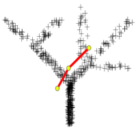
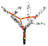
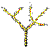
Iteration 1                     Iteration 5                     Iteration 50

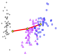
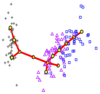
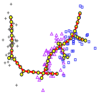
Iteration 1                     Iteration 10                     Iteration 50

Figure 1: Applying a simple “add a node to a node or bisect an edge” grammar to construct principal elastic trees (one node is added per iteration). Upper row: an example of two-dimensional branching distribution of points. Lower row: the classical benchmark, the “iris” four-dimensional dataset (point shapes distinguish three classes of points), the dataset and principal tree are presented in projection onto the plane of first two principal components.

The next problem is the elastic graph construction. Here we should find a compromise between simplicity of graph topology, simplicity of geometrical form for a given topology, and accuracy of approximation. Geometrical complexity is measured by the graph energy $U^{\phi}{(G)}$, and the error of approximation is measured by the energy of approximation $U^{\phi}_{A}(G,D)$. Both are included in the energy $U^{\phi}$. Topological complexity will be represented by means of elementary transformations: it is the length of the energetically optimal chain of elementary transformation from a given set applied to initial simple graph.

Graph grammars [11, 12] provide a well-developed formalism for the description of elementary transformations. An elastic graph grammar is presented as a set of production (or substitution) rules. Each rule has a form $A\to B$, where $A$ and $B$ are elastic graphs. When this rule is applied to an elastic graph, a copy of $A$ is removed from the graph together with all its incident edges and is replaced with a copy of $B$ with edges that connect $B$ to graph. For a full description of this language we need the notion of a labeled graph. Labels are necessary to provide the proper connection between $B$ and the graph.

A link in the energetically optimal transformation chain is constructed by finding a transformation application that gives the largest energy descent (after an optimization step), then the next link, and so on, until we achieve the desirable accuracy of approximation, or the limit number of transformations (some other termination criteria are also possible). The selection of an energetically optimal application of transformations by the trial optimization steps is time-consuming. There exist alternative approaches. The preselection of applications for a production rule $A\to B$ can be done through comparison of energy of copies of $A$ with its incident edges and stars in the transformed graph $G$.

As the simple (but already rather powerful) example we use a system of two transformations: “add a node to a node” and “bisect an edge.” These transformations act on a class of primitive elastic graphs: all non-terminal nodes with $k$ edges are centers of elastic k-stars, which form all the $k$-stars of the graph. For a primitive elastic graph, the number of stars is equal to the number of non-terminal nodes – the graph topology prescribes the elastic structure.

The transformation “add a node” can be applied to any vertex $y$ of $G$: add a new node $z$ and a new edge $(y,z)$. The transformation “bisect an edge” is applicable to any pair of graph vertices $y,y^{\prime}$ connected by an edge $(y,y^{\prime})$: Delete edge $(y,y^{\prime})$, add a vertex $z$ and two edges, $(y,z)$ and $(z,y^{\prime})$. The transformation of elastic structure (change in the star list) is induced by the change of topology, because the elastic graph is primitive. This two–transformation grammar with energy minimization builds principal trees (and principal curves, as a particular case) for datasets. A couple of examples are presented on Fig. 1. For applications, it is useful to associate one-dimensional continuums with these principal trees. Such a continuum consists of node images $\phi(y)$ and of pieces of straight lines that connect images of linked nodes.

3 Factorization and transformation of factors

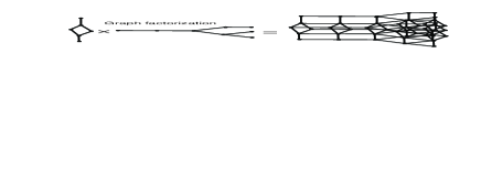
Figure 2: The Cartesian product of graphs.

If we approximate multidimensional data by a $k$-dimensional object, the number of points (or, more general, elements) in this object grows with $k$ exponentially. This is an obstacle for grammar–based algorithms even for modest $k$, because for analysis of the rule $A\to B$ applications we should investigate all isomorphic copies of $A$ in $G$. The natural way to avoid this obstacle is the principal object factorization. Let us represent an elastic graph as a Cartesian product of graphs (Fig. 2). Cartesian products $G_{1}\times\ldots\times G_{r}$ of elastic graphs $G_{1},\ldots G_{r}$ is an elastic graph with the vertex set $V_{1}\times\ldots\times V_{r}$. Let $1\leq i\leq r$ and $v_{j}\in V_{j}$ ($j\neq i$). For this set of vertices, $\{v_{j}\}_{j\neq i}$, a copy of $G_{i}$ in $G_{1}\times\ldots\times G_{r}$ is defined with vertices $(v_{1},\ldots v_{i-1},v,v_{i+1},\ldots v_{r})$ ($v\in V_{i}$), edges $((v_{1},\ldots v_{i-1},v,v_{i+1},\ldots v_{r}),(v_{1},\ldots v_{i-1},v^{\prime},v_{i+1},\ldots v_{r}))$ ($(v,v^{\prime})\in E_{i}$) and, similarly, $k$-stars of the form $(v_{1},\ldots v_{i-1},S_{k},v_{i+1},\ldots v_{r})$, where $S_{k}$ is a $k$-star in $G_{i}$. For any $G_{i}$ there are $\prod_{j,j\neq i}|V_{j}|$ copies of $G_{i}$ in $G$. Sets of edges and $k$-stars for Cartesian product are unions of that set through all copies of all factors. A map $\phi:V_{1}\times\ldots\times V_{r}\to R^{m}$ maps all the copies of factors into $R^{m}$ too. Energy of the elastic graph product is the energy sum of all factor copies. It is, of course, a quadratic functional of $\phi$.

The only difference between the construction of general elastic graphs and factorized graphs is in application of transformations. For factorized graphs, we apply them to factors. This approach significantly reduces the amount of trials in selection of optimal application. The simple grammar with two rules, “add a node to a node or bisect an edge,” is also powerful here, it produces products of primitive elastic trees. For such a product, the elastic structure is defined by the topology of the factors.

4 Conclusion: adaptive dimension and principal cubic complexes

In the continuum representation, factors are one-dimension continuums, hence, a product of $r$ factors is represented as an $r$-dimensional cubic complex [13] that is glued together from $r$-dimensional parallelepipeds (“cubes”). Thus, the factorized principal elastic graphs generate a new and, as we can estimate now, a useful construction: a principal cubic complex. One of the obvious benefits from this construction is adaptive dimension: the grammar approach with energy optimization develops the necessary number of non-trivial factors, and not more. These complexes can approximate multidimensional datasets with complex, but still low-dimensional topology. The topology of the complex is not prescribed, but adaptive. In that sense, they are even more flexible than SOMs. The whole approach can be interpreted as a intermediate between absolutely flexible neural gas [14] and significantly more restrictive elastic map [9]. It includes as simple limit cases the $k$-means clustering algorithm (low elasticity moduli) and classical PCA (high $\mu$ for $S_{2}$ and $\mu\to\infty$ for $S_{k}$, $k>2$).

References

- [1] T. Kohonen, Self-organized formation of topologically correct feature maps, Biological Cybernetics 43 (1982), 59–69.
- [2] T. Hastie,W. Stuetzle, Principal curves, Journal of the American Statistical Association 84(406) (1989), 502–516.
- [3] E. Erwin, K. Obermayer, K. Schulten, Self-organizing maps: ordering, convergence properties and energy functions, Biological Cybernetics 67 (1992), 47–55.
- [4] F. Mulier, V. Cherkassky, Self-organization as an iterative kernel smoothing process, Neural Computation 7 (1995), 1165–1177.
- [5] H. Ritter, T. Martinetz, K. Schulten, Neural Computation and Self-Organizing Maps: An Introduction. Addison-Wesley Reading, Massachusetts, 1992.
- [6] B. Kégl, A. Krzyzak, Piecewise linear skeletonization using principal curves, IEEE Transactions on Pattern Analysis and Machine Intelligence 24(1) (2002), 59–74.
- [7] A.N. Gorban, A.A. Rossiev, Neural network iterative method of principal curves for data with gaps, Journal of Computer and System Sciences International 38 (5) (1999), 825–831.
- [8] A. Zinovyev, Visualization of Multidimensional Data, Krasnoyarsk State University Press Publ., 2000, pp. 1–168.
- [9] A. Gorban, Y. Zinovyev, Elastic Principal Graphs and Manifolds and their Practical Applications, Computing 75 (2005), 359–379.
- [10] A. Gusev, Finite element mapping for spring network representations of the mechanics of solids, Phys. Rev. Lett. 93(2) (2004), 034302.
- [11] M. Nagl, Formal languages of labelled graphs, Computing 16 (1976), 113–137
- [12] M. Löwe, Algebraic approach to single–pushout graph transformation, Theor. Comp. Sci. 109 (1993), 181–224.
- [13] S. Matveev, M. Polyak, Cubic complexes and finite type invariants, In: Geometry & Topology Monographs, Volume 4: Invariants of knots and 3-manifolds, Kyoto, 2001, 215–233.
- [14] T. M. Martinetz, S. G. Berkovich, and K. J. Schulten. Neural-gas network for vector quantization and its application to time-series prediction. IEEE Transactions on Neural Networks, 4, 4 (1993), 558–569.