Convex Separation from Optimization via Heuristics

Abstract

Let $K$ be a full-dimensional convex subset of $\mathbb{R}^{n}$. We describe a new polynomial-time Turing reduction from the weak separation problem for $K$ to the weak optimization problem for $K$ that is based on a geometric heuristic. We compare our reduction, which relies on analytic centers, with the standard, more general reduction.

1 Introduction

Let $K$ be a full-dimensional convex subset of $\mathbb{R}^{n}$ containing a ball of finite radius centered at $c_{0}$ and contained in a ball of finite radius $R$. The separation problem for $K$ is that of finding a hyperplane that separates a given point $p$ from $K$, or concluding that $p\in K$. The separation problem is quite general in that it has been shown to be polynomial-time equivalent to other natural convex programming problems GLS88 . One of these problems is the optimization problem, which is the problem of maximizing a linear functional $c^{T}x$ over all $x\in K$ for a given $c\in\mathbb{R}^{n}$.

It may arise in some applications that solving the optimization problem for $K$ is more practically feasible than solving the separation problem directly, for example, if the extreme points of $K$ are parameterized by a number of parameters that is significantly smaller than $n$. In such a case, it might make sense to solve an instance of the separation problem by solving polynomially many instances of the optimization problem, using a Turing reduction GJ79 from separation to optimization. Despite this practical philosophy, which the authors have adopted with some success to the (NP-hard Gur03 ) quantum separability problem ITCE04 ; qphIoa05 , the main purpose of research into polynomial-time reductions among convex body problems is theoretical – to uncover the intrinsic beauty of the subject of convex programming algorithms, which historically marries physical intuition and mathematical rigor in a unique way. Our heuristics-based reduction is a fine example of this marriage.

2 Convex Body Problems and Cutting-plane Feasibility Algorithms

Let $S(K,\delta)$ denote the union of all balls of radius $\delta$ with centers belonging to $K$, and let $S(K,-\delta)$ denote the union of all centers of all balls of radius $\delta$ contained in $K$, where the balls are defined with respect to the Euclidean norm. We now give the formal definitions of the basic convex body problems that will concern us, taken from GLS88 .

Definition 1 (Weak Optimization Problem for $K$ (WOPT($K$)))

Given a rational vector $c\in\mathbb{R}^{n}$ and rational $\epsilon>0$, either

• find a rational vector $y\in\mathbb{R}^{n}$ such that $y\in S(K,\epsilon)$ and $c^{T}x\leq c^{T}y+\epsilon$ for every $x\in K$; or

• assert that $S(K,-\epsilon)$ is empty.

Definition 2 (Weak Separation Problem for $K$ (WSEP($K$)))

Given a rational vector $p\in\mathbb{R}^{n}$ and rational $\delta>0$, either

• assert $p\in S(K,\delta)$,   or

• find a rational vector $c\in\mathbb{R}^{n}$ with $||c||_{\infty}=1$ such that $c^{T}x<c^{T}p$ for every $x\in K$.

Let $K^{\prime}$ be a full-dimensional bounded convex subset of $\mathbb{R}^{n}$.

Definition 3 (Weak Violation Problem for $K^{\prime}$ (WVIOL($K^{\prime}$)))

Given a rational vector $c\in\mathbb{R}^{n}$ and rationals $\gamma$ and $\epsilon^{\prime}>0$, either

• assert that $c^{T}x\leq\gamma+\epsilon^{\prime}$ for all $x\in S(K^{\prime},-\epsilon^{\prime})$, or

• find a vector $y\in S(K^{\prime},\epsilon^{\prime})$ with $c^{T}y\geq\gamma-\epsilon^{\prime}$.

If $\gamma=-1$ and $c$ is the origin $\bar{0}\in\mathbb{R}^{n}$, then WVIOL($K^{\prime}$) reduces to the weak feasibility problem for $K^{\prime}$, denoted WFEAS($K^{\prime}$). By taking $\delta$, $\epsilon$, and $\epsilon^{\prime}$ to be zero, we implicitly define the corresponding strong problems, denoted SSEP, SOPT, SVIOL, and SFEAS. Note that SFEAS($K^{\prime}$) is the problem of deciding whether $K^{\prime}$ is empty or finding a point in $K^{\prime}$.

Central to our reduction are cutting-plane algorithms for WFEAS($K^{\prime}$), relative to a WSEP($K^{\prime}$) oracle $\mathcal{O}_{\text{\tiny{SSEP}($K^{\prime}$)}}$. All such algorithms have the same basic structure:

1. Define a (possibly very large) regular bounded convex set $P_{0}$ which is guaranteed to contain $K^{\prime}$, such that, for some reasonable definition of “center”, the center $\omega_{0}$ of $P_{0}$ is easily computed. The set $P_{0}$ is called an outer approximation to $K^{\prime}$. Common choices for $P_{0}$ are the origin-centered hyperbox, $\{x\in\mathbb{R}^{n}:-2^{L}\leq x_{i}\leq 2^{L},\hskip 5.69054pt1\leq i\leq n\}$ and the origin-centered hyperball, $\{x:x^{T}x\leq 2^{L}\}$ (where $2^{L}$ is a trivially large bound).

2. Give the center $\omega$ of the current outer approximation $P$ to $\mathcal{O}_{\text{\tiny{SSEP}($K^{\prime}$)}}$.

3. If $\mathcal{O}_{\text{\tiny{SSEP}($K^{\prime}$)}}$ asserts “$\omega\in K^{\prime}$”, then HALT.

4. Otherwise, say $\mathcal{O}_{\text{\tiny{SSEP}($K^{\prime}$)}}$ returns the hyperplane $\pi_{c,b}$ such that $K^{\prime}\subset\{x:c^{T}x\leq b\}$. Update (shrink) the outer approximation $P:=P\cap\{x:c^{T}x\leq b^{\prime}\}$ for some $b^{\prime}\geq b$. Possibly perform other computations to further update $P$. Check stopping conditions; if they are met, then HALT. Otherwise, go to step (ii).

The difficulty with such algorithms is knowing when to halt in step (iv). Generally, the stopping conditions are related to the size of the current outer approximation. Because it is always an approximate (weak) feasibility problem that is solved, the associated accuracy parameter $\epsilon^{\prime}$ can be exploited to get a “lower bound” $V$ on the “size” of $K^{\prime}$, with the understanding that if $K^{\prime}$ is smaller than this bound, then the algorithm can correctly assert that $S(K^{\prime},-\epsilon^{\prime})$ is empty. Thus the algorithm stops in step (iv) when the current outer approximation is smaller than $V$.

The cutting-plane algorithm is called (oracle-) polynomial-time if it runs in time $O(\textrm{poly}(n,\log(R^{\prime}/\epsilon^{\prime})))$ with unit cost for the oracle, where $R^{\prime}$ is the outer radius of $K^{\prime}$. It is called (oracle-) fully polynomial if it runs in time $O(\textrm{poly}(n,R^{\prime}/\epsilon^{\prime}))$.

There are a number of such polynomial-time convex feasibility algorithms (see AV95 for a discussion of all of them). The three most important are the ellipsoid method, the volumetric center method, and the analytic center method. The ellipsoid method has $P_{0}=\{x:x^{T}x\leq 2^{L}\}$ and is the only one which requires “further update” of the outer approximation $P$ in step (iv) after a cut has been made – a new minimal-volume ellipse is drawn around $P:=P\cap\{x:c^{T}x\leq b^{\prime}\}$. The ellipsoid method, unfortunately, suffers badly from gigantic precision requirements, making it practically unusable. The volumetric center and analytic center algorithms are more efficient than the ellipsoid algorithm and are very similar to each other in complexity and precision requirements, with the analytic center algorithm having some supposed practical advantages.

The cutting plane $\{x:c^{T}x=b^{\prime}\}$ requires further definition:

$$\textrm{If }\left\{\begin{array}[]{rcl}b^{\prime}&<&c^{T}\omega\\ b^{\prime}&=&c^{T}\omega\\ b^{\prime}&>&c^{T}\omega\end{array}\right\}\textrm{ then the above is a }\left\{\begin{array}[]{c}\textrm{\emph{deep-cut}}\\ \textrm{\emph{central-cut}}\\ \textrm{\emph{shallow-cut}}\end{array}\right\}\textrm{ algorithm.}$$ (1)

Intuitively, deep-cut algorithms should be fastest. Ironically, though, except for the case of ellipsoidal algorithms (which are practically inefficient), the algorithms that are provably polynomial-time are central- or even shallow-cut algorithms.

3 Reduction via Heuristics

Assume without loss that $c_{0}=\bar{0}$. Our goal is to develop a new oracle-polynomial-time algorithm for WSEP($K$) with respect to an oracle for WOPT($K$) (running in time $O(\textrm{poly}(n,\log(R/\delta)))$). We do this via a geometric approach, which differs from the standard approach covered in the next section. In this section, we ignore the weakness of the separation and optimization problems, as it obfuscates the main ideas; that is, we assume we are solving SSEP($K$) with an oracle for SOPT($K$).

Suppose we have an oracle $\mathcal{O}_{\text{\tiny{SOPT}($K$)}}$ for the optimization problem over $K$ such that, given a nonzero input vector $c$, $\mathcal{O}_{\text{\tiny{SOPT}($K$)}}$ outputs a point $\mathcal{O}_{\text{\tiny{SOPT}($K$)}}(c)\\ \equiv k_{c}\in K$ that maximizes $c^{T}x$ for all $x\in K$. An important step in developing the algorithm is noting that, given $\mathcal{O}_{\text{\tiny{SOPT}($K$)}}$, the search for a separating hyperplane reduces to the search for a region on the $(n-1)$-dimensional surface of the unit hypersphere $S_{n}$ (embedded in $\mathbb{R}^{n}$) centered at the origin. For $p\notin K$, this region $M_{p}$ is simply $\{c\in S_{n}:\hskip 5.69054ptc^{T}k_{c}<c^{T}p\}$ (see Figure 1).

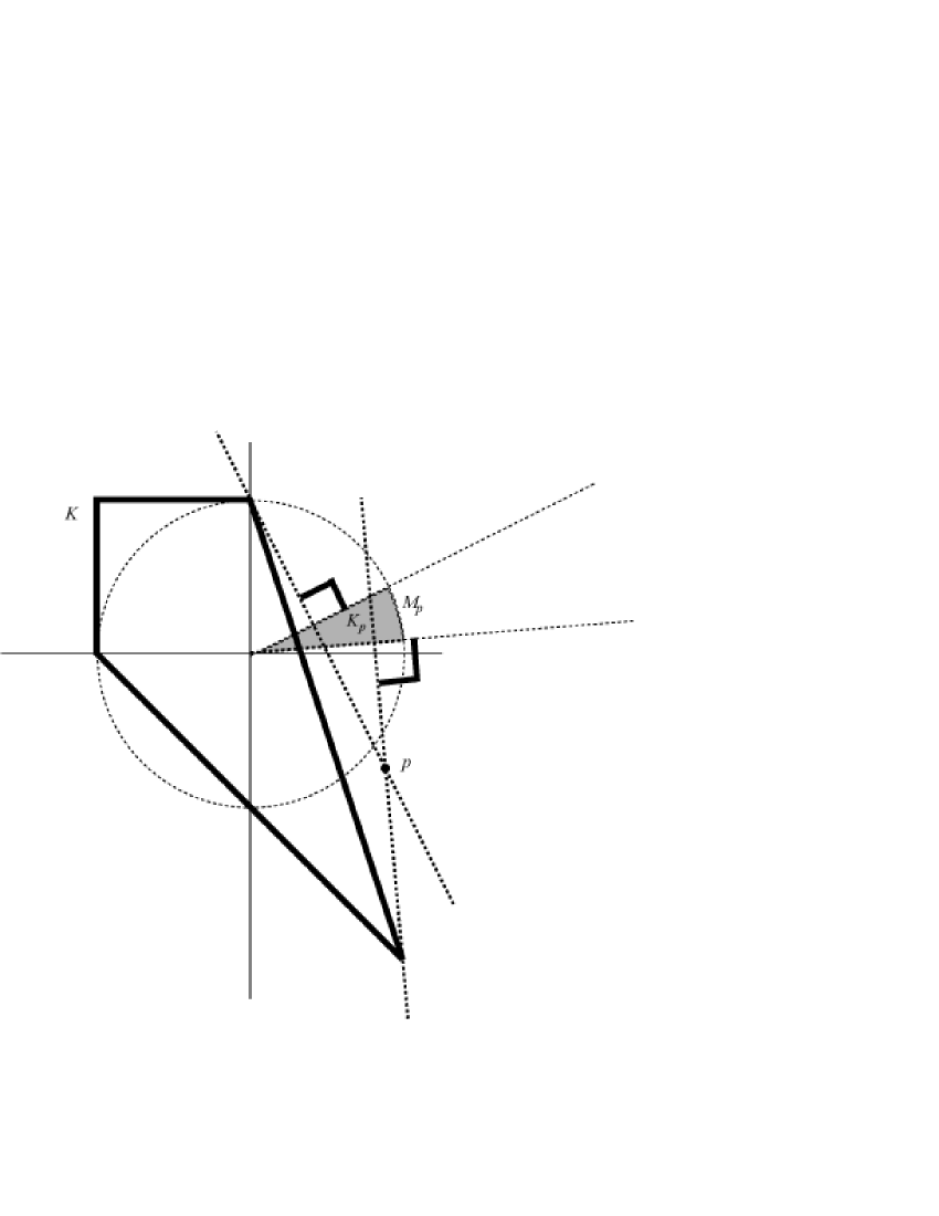
Figure 1: The sets $M_{p}$ and $K_{p}$ in $\mathbb{R}^{2}$. Pictured in heavy outline is a set $K$ in $\mathbb{R}^{2}$, where $K:=\mathrm{conv}\{(0,1),(-1,1),(-1,0),(1,-2)\}$. A point $p=(-7/8,-3/4)$ is shown as a heavy dot. The unit circle is drawn in a dashed line. The set $M_{p}$ is the arc of the unit circle that the shaded pie-slice subtends; the set $K_{p}$ is the shaded pie-slice. In two dimensions, the set $M_{p}$ ($K_{p}$) is easy to construct. This construction has been illustrated: draw the two distinct lines through $p$ that are tangent to $K$; the lines that determine the pie-slice are the two straight lines that are perpendicular to the lines through $p$.

The first observation is that, since $K$ properly contains the origin, $M_{p}$ is contained in the hemisphere defined by $\{x:p^{T}x\geq 0\}$:

Fact 3.1

For all $m\in M_{p}$, $m^{T}p>0$.

Proof

Let $m\in M_{p}$. Then $m^{T}p>m^{T}k$ for all $k\in K$. But the fact that the 0-vector is properly contained in $K$ implies that there exists $k\in K$ such that $m^{T}k>0$.

The second observation, Lemma 1, is based on the following heuristic, which can be pictured in $\mathbb{R}^{2}$ and $\mathbb{R}^{3}$. Suppose $c$, $||c||=1$, is not in $M_{p}$ (but is reasonably close to $M_{p}$) and that the oracle returns $k_{c}$. What is a natural way to modify the vector $c$, so that it gets closer to $M_{p}$? Intuition dictates moving $c$ away from $k_{c}$ and towards $p$, that is, add a small component of the vector $(p-k_{c})$ to $c$, in order to generate a new guess $c^{\prime}=c+\lambda(p-k_{c})/||p-k_{c}||$, for some $\lambda>0$, which we could then give to the oracle again (see Figure 2). Incidentally, we have found that the following little program, which embodies this heuristic, actually performs well:

• $c:=p/||p||;\hskip 5.69054ptd:=1;\hskip 5.69054pti:=0;$ • while  $(d>0$  and  $i<N)$  do  $\{$ • $k_{c}:=\mathcal{O}_{\text{\tiny{SOPT}($K$)}}(c);$ • $d:=c^{T}k_{c}-c^{T}p;$ • if$\hskip 5.69054pt(d<0)$  then  $\{$ return $c$ $\}$ • else  $\{$ $c:=c+d(p-k_{c})/||p-k_{c}||$;  $c:=c/||c||$;  $i:=i+1\}\};$ • return “INCONCLUSIVE”

This program can be regarded as an extremely simple heuristic for the separation problem when given an optimization subroutine (of course, it may give inconclusive results; in practice, one should set $N$ as large as is practically feasible).

Interestingly, the above heuristic can be formalized as follows. If $c$ is not in $M_{p}$ but is sufficiently close to $M_{p}$, then $c$, $p$, and $k_{c}$ can be used to define a hemisphere which contains $M_{p}$ and whose great circle cuts through $c$. More precisely:

Lemma 1

Suppose $m\in M_{p}$, $c\notin M_{p}$, and let $\bar{a}:=(p-k_{c})-\mathrm{Proj}_{c}(p-k_{c})$. If $m^{T}c\geq 0$ then $m^{T}\bar{a}>0$.

Proof

Note that $m^{T}\bar{a}=m^{T}(p-k_{c})-[c^{T}(p-k_{c})](m^{T}c)$. The hypotheses of the lemma immediately imply that $m^{T}(p-k_{c})>0$ and $c^{T}(p-k_{c})\leq 0$. Thus, if $m^{T}c\geq 0$, then $m^{T}\bar{a}>0$.

The lemma gives a method for reducing the search space after each query to $\mathcal{O}_{\text{\tiny{SOPT}($K$)}}$ by giving a cutting plane $\{x:\bar{a}^{T}x=0\}$ that slices off a portion of the search space.

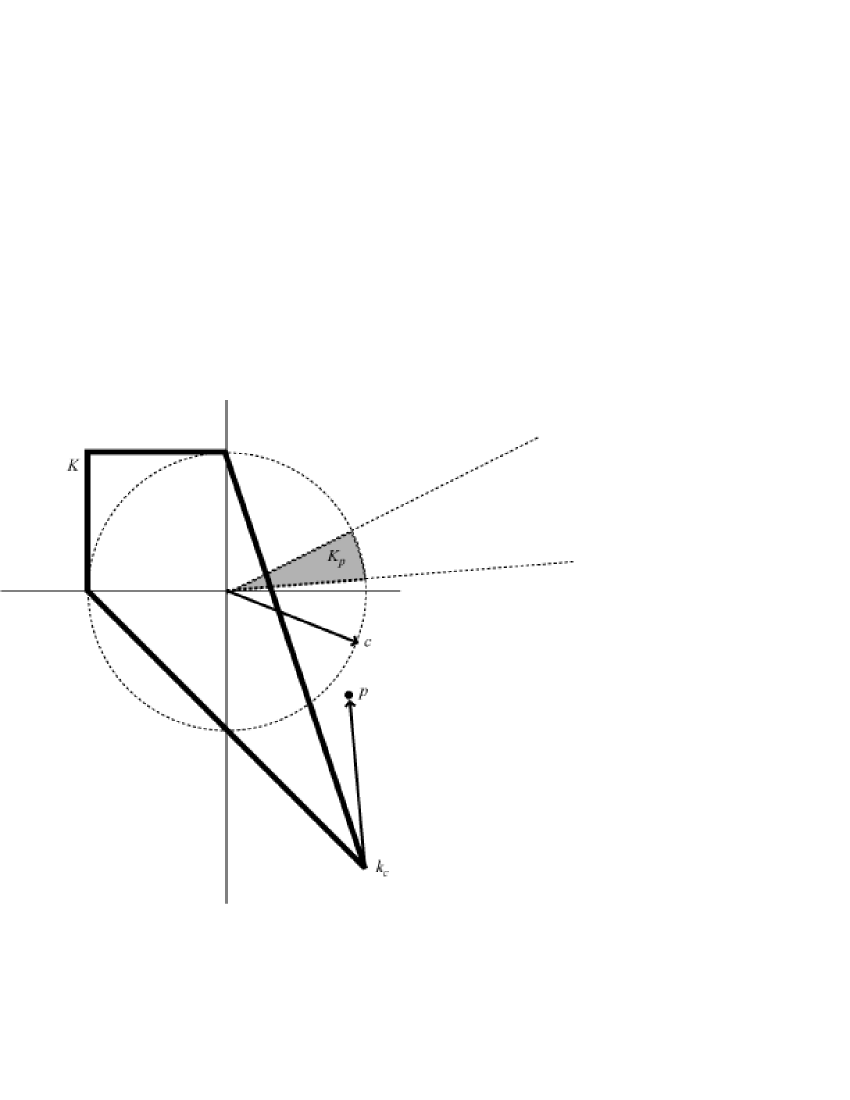
Figure 2: Illustration of heuristic behind Lemma 1. Continuing from Figure 1, the unit vector $c$ is a test vector that is close to $M_{p}$ but not in $M_{p}$. Evidently, adding a component of $(p-k_{c})$ to $c$ moves it closer to $M_{p}$. This intuition also holds in $\mathbb{R}^{3}$.

Our search problem can easily be reduced to an instance of SFEAS($K^{\prime}$), where $K^{\prime}$ is

$$K_{p}:=\left[\mathrm{ConvexHull}\left(M_{p}\cup\{\bar{0}\}\right)\right]\setminus\{\bar{0}\}.$$ (2)

The set $K_{p}$, if not empty, can be viewed as a cone-like object, emanating from the origin and cut off by the unit hypersphere (see Figure 1). The oracle $\mathcal{O}_{\text{\tiny{SOPT}($K$)}}$, along with Lemma 1, essentially gives a separation oracle for $K_{p}$, as long as the test vectors $c$ given to $\mathcal{O}_{\text{\tiny{SOPT}($K$)}}$ satisfy

$$\text{$m^{T}c\geq 0$ for all $m\in M_{p}$}.$$ (3)

How could we ensure that all our test vectors $c$ satisfy (3)? Recall Fact 3.1, which says that the set $K_{p}$ is contained in the halfspace $\{x:p^{T}x\geq 0\}$. Let $B_{n}$ be the origin-centered unit hyperball in $\mathbb{R}^{n}$ and let $a_{1}:=p/||p||$. Thus, straight away, the search space is reduced to the hemisphere $B_{n}\cap\{x:a_{1}^{T}x\geq 0\}$. The first test vector to give to the oracle $\mathcal{O}_{\text{\tiny{SOPT}($K$)}}$ is $p/||p||$, which clearly has nonnegative dot-product with all points in $K_{p}$ and hence all $m\in M_{p}$. By way of induction, assume that, at some later stage in the algorithm, the current search space has been reduced to $P:=B_{n}\bigcap\cap_{i=1}^{h}\{x:a_{i}^{T}x\geq b_{i}\}$ by the generation of cutting planes $\{x:a_{i}^{T}x=b_{i}\}$, where the $a_{i}$, for $i=2,3,\ldots,h$, are the normalized $\bar{a}$ from $h-1$ invocations of Lemma 1. Let $\omega$ be the “center” of $P$, and suppose that this “center” is a positive linear (conic) combination of the normal vectors $a_{i}$, that is,

$$\omega=\sum_{i=1}^{h}\lambda_{i}a_{i},\hskip 5.69054pt\textrm{where $\lambda_{i}\geq 0$ for all $i=1,2,\ldots,h$.}$$ (4)

Then, by inductive hypothesis, this implies that $m^{T}\omega\geq 0$ for all $m\in M_{p}$. Thus, $c:=\omega/||\omega||$ is a suitable vector to give to the oracle $\mathcal{O}_{\text{\tiny{SOPT}($K$)}}$ and use in Lemma 1. Therefore, it suffices to find a definition of “center $\omega$ of $P$” that satisfies (4), in order that all our test vectors $c$ satisfy (3). Because we require (3), none of the feasibility algorithms mentioned in Section 2 can be applied directly. However, the analytic-center algorithm due to Atkinson and Vaidya AV95 beautifully lends itself to a modification that allows (3) to be satisfied.

Reducing the separation problem for $K$ to the convex feasibility problem for some $K^{\prime}$, while using the optimization oracle for $K$ as a separation oracle for $K^{\prime}$, is not a new concept in convex analysis. But the precise way that Lemma 1 generates each new cutting plane, incorporating the correction-heuristic, does not appear in the literature. This is likely because there is a more general way to carry out such a reduction, covered in the next section, which does not require (4).

4 Comparison to Standard Reduction

Note that our reduction requires knowledge of $c_{0}$ and $R$. A polynomial-time Turing reduction from WSEP($K$) to WOPT($K$) is well known – even when $c_{0}$ and $R$ are unknown. One such (ellipsoidal) reduction is given in Theorem 4.4.7 in GLS88 ; however, it may be more general than is necessary. If $R$ is known, then the standard way to perform the reduction of the previous section may be found in the synthesis of Lemma 4.4.2 and Theorem 4.2.2 in GLS88 ; we outline it in the following paragraph.

Definition 4 (Polar of $K$)

The polar $K^{\star}$ of a full-dimensional convex set $K\subset\mathbb{R}^{n}$ that contains the origin is defined as

$$K^{\star}:=\{c\in\mathbb{R}^{n}:c^{T}x\leq 1\hskip 5.69054pt\forall x\in K\}.$$ (5)

If $c\in K^{\star}$, then the plane $\pi_{c,1}\equiv\{x:c^{T}x=1\}$ separates $p\in\mathbb{R}^{n}$ from $K$ when $c^{T}p>1$. Thus, the separation problem for $p$ is equivalent to the feasibility problem for $Q_{p}$, defined as

$$Q_{p}:=K^{\star}\cap\{c:p^{T}c\geq 1\}.$$ (6)

As mentioned in the previous section (and elaborated on in the next section), to solve the feasibility problem for any $K^{\prime}$, it suffices to have a separation routine for $K^{\prime}$. Because we can easily build a separation routine $\mathcal{O}_{\text{\tiny{SSEP}($Q_{p}$)}}$ for $Q_{p}$ out of $\mathcal{O}_{\text{\tiny{SSEP}($K^{\star}$)}}$, it suffices to have a separation routine $\mathcal{O}_{\text{\tiny{SSEP}($K^{\star}$)}}$ for $K^{\star}$ in order to solve the feasibility problem for $Q_{p}$. Building $\mathcal{O}_{\text{\tiny{SSEP}($Q_{p}$)}}$ out of $\mathcal{O}_{\text{\tiny{SSEP}($K^{\star}$)}}$ is done as follows:

Routine $\mathcal{O}_{\text{\tiny{SSEP}($Q_{p}$)}}(y)$:
case: $p^{T}y<1$
return $-p$
else: $p^{T}y\geq 1$
call $\mathcal{O}_{\text{\tiny{SSEP}($K^{\star}$)}}(y)$
case: $\mathcal{O}_{\text{\tiny{SSEP}($K^{\star}$)}}(y)$ returns separating vector $q$
return $q$
else: $\mathcal{O}_{\text{\tiny{SSEP}($K^{\star}$)}}(y)$ asserts $y\in K^{\star}$
return “$y\in Q$”

It remains to show that the optimization routine $\mathcal{O}_{\text{\tiny{SOPT}($K$)}}$ for $K$ gives a separation routine $\mathcal{O}_{\text{\tiny{SSEP}($K^{\star}$)}}$ for $K^{\star}$. Suppose $y$ is given to $\mathcal{O}_{\text{\tiny{SOPT}($K$)}}$, which returns $k\in K$ such that $y^{T}x\leq y^{T}k=:b$ for all $x\in K$. If $b\leq 1$, then $\mathcal{O}_{\text{\tiny{SSEP}($K^{\star}$)}}$ may assert $y\in K^{\star}$. Otherwise, $\mathcal{O}_{\text{\tiny{SSEP}($K^{\star}$)}}$ may return $k$, because $\pi_{k,1}$ (and hence $\pi_{k,b}$) separates $y$ from $K^{\star}$: since $k^{T}y=b>1$, it suffices to note that $k^{T}c=c^{T}k\leq 1$ for all $c\in K^{\star}$ by the definition of $K^{\star}$ and the fact that $k\in K$.

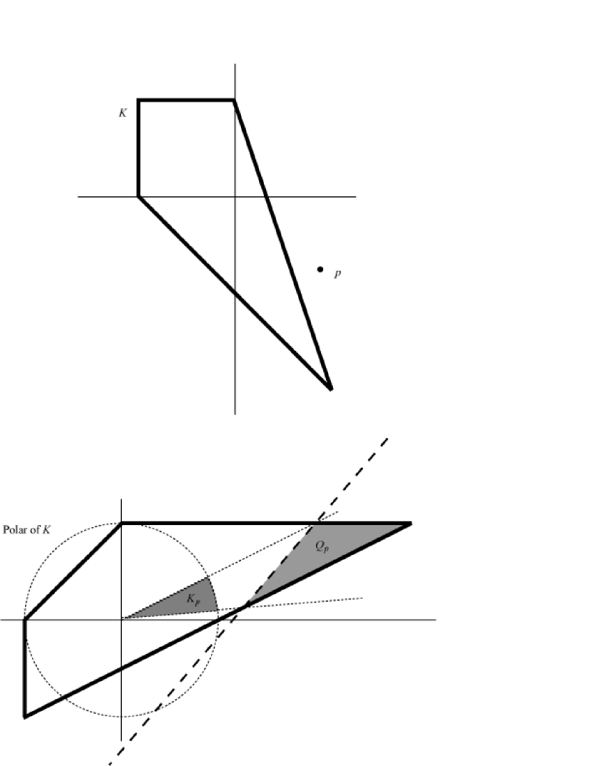
Figure 3: The upper picture is a set $K$ in $\mathbb{R}^{2}$, where $K:=\mathrm{conv}\{(0,1),(-1,1),(-1,0),(1,-2)\}$. A point $p=(-7/8,-3/4)$ is shown. The polar $K^{\star}$ of $K$ is shown in heavy outline in the lower picture; $K^{\star}=\mathrm{conv}\{(0,1),(-1,0),(-1,-1),(3,1)\}$. The set $Q_{p}$ is the shaded polytope, bounded by the long-dashed plane $\{c:p^{T}c=1\}$. The set $K_{p}$ is the shaded pie-slice and is the radial projection of $Q_{p}$ onto $B_{n}$ (whose boundary is shown as a short-dashed circle). The particular $K$ and $K^{\star}$ are taken from NW88 .

Figure 3 shows the relationship between the method of Section 3 and the above method, by illustrating that the set $K_{p}$ (defined in (2)) is just the radial projection of $Q_{p}$ onto $B_{n}$. Using “$A\longrightarrow B$” to mean “$B$ Turing-reduces to $A$”, the standard reduction chain is

$$\textrm{WOPT}(K)\longrightarrow\textrm{WSEP}(K^{\star})\overset{R}{\longrightarrow}\textrm{WSEP}(Q_{p})\longrightarrow\textrm{WFEAS}(Q_{p}),$$ (7)

where we indicate that the middle reduction requires knowledge of outer radius $R$. Our reduction, which is substantially less general, may be written

$$\textrm{WOPT}(K)\longrightarrow\textrm{WSEP}(K_{p})\Bigl{.}\Bigr{|}_{(\ref{HypothesisOfDonnyLemma})}\overset{R,c_{0}}{\underset{(\ref{eqn_CenterIsConicCombinationOfNormals})}{\longrightarrow}}\textrm{WFEAS}(K_{p}),$$ (8)

where the weak separation problem has been restricted (queries must satisfy the condition (3) of Lemma 1) and we note that the rightmost link requires, in addition to knowledge of $R$ and $c_{0}$, a WFEAS algorithm whose centers satisfy (4) (see Section 5).

The two reductions have similar structure; the novelty of our reduction lies in the way the cutting planes are generated, which is based on the heuristic: if the center $\omega$ satisfies (4), then cutting near $\omega$ pushes the new center in the direction of the normal of the new cutting plane; but this direction is essentially $(p-k_{c})$ (except with the projection onto $c$ removed). Note that the normal of every new cutting plane depends on the given point $p$, whereas in the standard reduction it does not. These attributes tempt us to conjecture that our reduction performs “better” in practice when $p\notin K$ (though not in any significant asymptotic sense).

Note that, even though $\mathcal{O}_{\text{\tiny{SSEP}($K^{\star}$)}}$, built on $\mathcal{O}_{\text{\tiny{SOPT}($K$)}}$, gives deep cuts $\pi_{k,1}$, it is not known how to utilize the deep cuts to get a polynomial-time algorithm using analytic or volumetric centers. Our cut-generation method in Section 3 is capable only of giving central cuts; but this does not, a priori, put it at any disadvantage (relative to the standard cut-generation method) with regard to polynomial-time analytic or volumetric center algorithms. In the next section, we briefly outline how our heuristic indeed yields a polynomial-time algorithm (justifying the Turing reduction in (8)).

5 Analytic Centers

Let $P$ be the current outer approximation $P:=B_{n}\bigcap\cap_{i=1}^{h}\{x:a_{i}^{T}x\geq b_{i}\}$, as described in the second-last paragraph of Section 3. Recall that we need a definition of “center $\omega$ of $P$” that satisfies (4). Define the analytic center $\omega$ of $P$ as the unique minimizer of the real convex function

$$F(x):=-\sum_{i=1}^{h}\log(a_{i}^{T}x-b_{i})-\log(1-x^{T}x).$$ (9)

The relation $\nabla F(\omega)=0$ gives

$$\omega=\frac{1-\omega^{T}\omega}{2}\sum_{i=1}^{h}\frac{a_{i}}{a_{i}^{T}\omega-b_{i}},$$ (10)

which shows that $\omega$, defined as the analytic center of $P$, indeed satisfies (4).

Our algorithm is a modification of the one in AV95 : we use a hypersphere for $P_{0}$ instead of a hyperbox (i.e. we adapt the analysis to handle a convex quadratic constraint). We refer to qphIoa05 for details (which rely on results in NN94 ; Ren01 ), but remind the reader of some of the algorithm’s characteristics. The algorithm stops when the current outer approximation becomes either too small (volume-wise) or too thin to contain $K_{p}$. For this, a lower bound $r>0$ on the radius of the largest ball contained in $K_{p}$ is needed. By exploiting the accuracy parameter $\delta$ of the weak separation problem, such an $r$ exists (and is derived in qphIoa05 ). The actual algorithm is not as straightforward. For instance, it is a shallow-cut algorithm ($b_{i}<0$) so as to keep the analytic center of the old $P$ in the new $P$ and the new center close to the old center. As well, cutting planes are occasionally discarded so that $h$ does not exceed some prespecified number.

Incidentally, it is an open problem whether there exists a polynomial-time, analytic center algorithm for the convex feasibility problem that does not require shallow cutting. It has been suggested by Mitchell Mit03 ; Mit05 that central cutting can be used in the Atkinson-Vaidya algorithm, if certain techniques from MT92 are employed to compute the new analytic center. However, from correspondence with Mitchell and Ye Ye05 , it is unclear whether modifying the Atkinson-Vaidya algorithm in this way retains the polynomial-time convergence: while it is clear that a new analytic center can be efficiently computed when central cuts are used, it is not clear that all the other delicate machinery in the convergence argument emerges unscathed. If central cuts may indeed be used, then the worst-case precision requirements of our algorithm are significantly reduced qphIoa05 .

6 Acknowledgements

We gratefully acknowledge an anonymous referee who pointed out the relationship between our reduction and the standard reduction, allowing us to streamline this paper and correctly identify its novel contribution. We also thank Tom Stace and Coralia Cartis for assistance. LMI acknowledges the support of GCHQ and ORS (UK), and NSERC (Canada); BCT acknowledges CMI (UK); DC acknowledges NSERC and the University of Waterloo.

References

- [1] M. Grötschel, L. Lovász, and A. Schrijver. Geometric algorithms and combinatorial optimization. Springer-Verlag, Berlin, 1988.
- [2] Michael R. Garey and David S. Johnson. Computers and Intractability: A Guide to the theory of NP-completeness. W.H. Freeman and Company, New York, 1979.
- [3] L. Gurvits. Classical deterministic complexity of Edmonds’ problem and quantum entanglement. In Proceedings of the thirty-fifth ACM symposium on Theory of computing, pages 10–19, New York, 2003. ACM Press.
- [4] M. Nielsen and I. Chuang. Quantum Computation and Quantum Information. Cambridge University Press, Cambridge, 2000.
- [5] L. M. Ioannou, B. C. Travaglione, D. C. Cheung, and A. K. Ekert. Improved algorithm for quantum separability and entanglement detection. Phys. Rev. A, 70:060303(R), 2004.
- [6] L. M. Ioannou. Computing finite-dimensional bipartite quantum separability, 2005. PhD thesis, available at http://arXiv.org/abs/cs/0504110.
- [7] David S. Atkinson and Pravin M. Vaidya. A cutting plane algorithm for convex programming that uses analytic centers. Mathematical Programming, 69:1–43, 1995.
- [8] G. L. Nemhauser and L.A. Wolsey. Integer and Combinatorial Optimization. John Wiley and Sons, Chichester, 1988.
- [9] Y. Nesterov and A. Nemirovskii. Interior-Point Polynomial Algorithms in Convex Programming. SIAM, Philadelphia, 1994.
- [10] J. Renegar. A Mathematical View of Interior-Point Methods in Convex Optimization. MPS-SIAM, Philadelphia, 2001.
- [11] J. E. Mitchell. Polynomial interior point cutting plane methods. Optimization Methods and Software, 18(5):507–534, 2003.
- [12] J. E. Mitchell. Private communication. 2005.
- [13] J. E. Mitchell and M. J. Todd. Solving combinatorial optimization problems using karmarkar’s algorithm. Mathematical Programming, 56:245–284, 1992.
- [14] Y. Ye. Private communication. 2005.