On the tree-transformation power of XSLT

Abstract

XSLT is a standard rule-based programming language for expressing transformations of XML data. The language is currently in transition from version 1.0 to 2.0. In order to understand the computational consequences of this transition, we restrict XSLT to its pure tree-transformation capabilities. Under this focus, we observe that XSLT 1.0 was not yet a computationally complete tree-transformation language: every 1.0 program can be implemented in exponential time. A crucial new feature of version 2.0, however, which allows node sets over temporary trees, yields completeness. We provide a formal operational semantics for XSLT programs, and establish confluence for this semantics.

1 Introduction

XSLT is a powerful rule-based programming language, relatively widely used, for expressing transformations of XML data, and is developed by the W3C (World Wide Web Consortium) [2, 8, 17]. An XSLT program is run on an XML document as input, and produces another XML document as output. (XSLT programs are actually called “stylesheets”, as one of their main uses is to produce stylised renderings of the input data, but we will continue to call them programs here.)

The language is actually in a transition period: the current standard, version 1.0, is being replaced by version 2.0. It is important to understand what the new features of 2.0 really add. In the present paper, we focus on the tree-transformation capabilities of XSLT. Indeed, XML documents are essentially ordered, node-labeled trees.

From the perspective of tree-transformation capabilities, the most important new feature is that of “node sets over temporary trees”. We will show that this feature turns XSLT into a computationally complete tree-transformation language. Indeed, as we will also show, XSLT 1.0 was not yet complete in this sense. Specifically, any 1.0 program can be implemented within exponential time in the worst case. Some programs actually express PSPACE-complete problems, because we will show that any linear-space turing machine can be simulated by an XSLT 1.0 program.

To put our results in context, we note that the designers of XSLT will most probably regard the incompleteness of their language as a feature, rather than a defect. Indeed, in the requirements document for 2.0, turning XSLT into a general-purpose programming language is explicitly stated as a “non-goal” [3]. In that respect, our result on the completeness of 2.0 exposes (albeit in a narrow sense) a failure to meet the requirements!

At this point we should be a little clearer on what we mean by “focusing on the tree-transformation capabilities of XSLT”. As already mentioned, XML documents are essentially trees where the nodes are labeled by arbitrary strings. We make abstraction of this string content by regarding the node labels as coming from some finite alphabet. Accordingly, we strip XSLT of its string-manipulation functions, and restrict its arithmetic to arbitrary polynomial-time functions on counters, i.e., integers in the range $\{1,2,\dots,n\}$ with $n$ the number of nodes in the input tree. It is, incidentally, quite easy to see that XSLT 1.0 without these restrictions can express all computable functions on strings (or integers). Indeed, rules in XSLT can be called recursively, and we all know that arbitrary recursion over the strings or the integers gives us completeness.

We will provide a formal operational semantics for the substantial fragment of XSLT discussed in this paper. A formal semantics has not been available, although the W3C specifications represent a fine effort in defining it informally. Of course we have tried to make our formalisation faithful to those specifications. Our semantics does not impose an order on operations when there is no need to, and as a result the resulting transition relation is non-deterministic. We establish, however, a confluence property, so that any two terminating runs on the same input yield the same final result. Confluence was not yet proven rigorously for XSLT, and can help in providing a formal justification for alternative processing strategies that XSLT implementations may follow for the sake of optimisation.

2 Data model

2.1 Data trees

Let $\Sigma$ be a finite alphabet, including the special label doc. By a data tree we simply mean a finite ordered tree, in which the nodes are labeled by elements of $\Sigma$. Up to isomorphism, we can describe a data tree $\mathbf{t}$ by a string $\mathit{string}(\mathbf{t})$ over the alphabet $\Sigma$ extended with the two symbols { and }: if the root of $\mathbf{t}$ is labeled a and its sequence of top-level subtrees is $\mathbf{t}_{1},\dots,\mathbf{t}_{k}$, then

$$\mathit{string}(\mathbf{t})=\texttt{a}\texttt{\char 123\relax}\mathit{string}(\mathbf{t}_{1})\dots\mathit{string}(\mathbf{t}_{k})\texttt{\char 125\relax}$$

Thus, for the data tree shown in Figure 1, the string representation equals

$$\texttt{a}\texttt{\char 123\relax}\texttt{b}\texttt{\char 123\relax}\texttt{\char 125\relax}\texttt{c}\texttt{\char 123\relax}\texttt{a}\texttt{\char 123\relax}\texttt{\char 125\relax}\texttt{b}\texttt{\char 123\relax}\texttt{\char 125\relax}\texttt{\char 125\relax}\texttt{c}\texttt{\char 123\relax}\texttt{\char 125\relax}\texttt{\char 125\relax}.$$

a b c a b c

Figure 1: A data tree.

A data forest is a finite sequence of data trees. Forests arise naturally in XSLT, and for uniformity reasons we need to be able to present them as data trees. This can easily be done as follows:

Definition 1 (maketree).

Let $F$ be a data forest. Then $\mathit{maketree}(F)$ is the data tree obtained by affixing a root node on top of $F$, and labeling this root node with doc.

2.2 Stores and values

Let $\mathcal{T}$ be a supply of tree variables, including the special tree variable Input. We define:

Definition 2.

A store is a finite set $\mathbf{S}$ of pairs of the form $(x,\mathbf{t})$, where $x\in\mathcal{T}$ and $\mathbf{t}$ is a data tree, such that (1) Input occurs in $\mathbf{S}$; (2) no tree variable occurs twice in $\mathbf{S}$; and (3) all data trees occurring in $\mathbf{S}$ have disjoint sets of nodes.

The tree assigned to Input is called the input tree; the other trees are called the temporary trees.

Definition 3.

A value over $\mathbf{S}$ is a finite sequence consisting of nodes from trees in $\mathbf{S}$, and counters over $\mathbf{S}$. Here, a counter over $\mathbf{S}$ is an integer in the range $\{1,2,\dots,n\}$, where $n$ is the total number of nodes in $\mathbf{S}$.

Values as defined above formalise the kind of values that can be returned by XPath expressions. XPath [1, 5] is a language that is used as a sublanguage in XSLT for the purpose of selecting nodes from trees. But XPath expressions can also return numbers, which is useful as an aid in making node selections (e.g., the $i$-th child of a node, or the $i$-th node of the tree in preorder). We limit these numbers to counters, in order to concentrate on pure tree transformations.

3 XPath abstraction

Since the language XPath is already well understood [27, 13, 7, 14], and its study in itself is not our focus, we will work with an abstraction of XPath, which we denote by $\mathcal{X}$. For our purposes it will suffice to divide the $\mathcal{X}$-expressions in only two different types, which we denote by nodes and mixed. A value is of type nodes if it consists exclusively of nodes; otherwise it is of type mixed.

In order to define the semantics of $\mathcal{X}$, we need some definitions, which reflect those from the XPath specification. Let $\mathcal{V}$ be a supply of value variables, disjoint from $\mathcal{T}$.

Definition 4.

An environment over $\mathbf{S}$ is a finite set $\mathbf{E}$ of pairs of the form $(x,v)$, where $x\in\mathcal{V}$ and $v$ is a value over $\mathbf{S}$, such that no value variable occurs twice in $\mathbf{E}$.

Definition 5.

A context triple over $\mathbf{S}$ is a triple $(z,i,k)$ where $z$ is a node from $\mathbf{S}$ or a counter over $\mathbf{S}$, and $i$ and $k$ are counters over $\mathbf{S}$ such that $i\leqslant k$. We call $z$ the context item, $i$ the context position, and $k$ the context size.

Definition 6.

A context is a triple $(\mathbf{S},\mathbf{E},c)$ where $\mathbf{S}$ is a store, $\mathbf{E}$ is an environment over $\mathbf{S}$, and $c$ is a context triple over $\mathbf{S}$.

If we denote the universe of all possible contexts by Contexts, the semantics of $\mathcal{X}$ is now given by a partial function $\mathit{eval}$ on $\mathcal{X}\times\mathit{Contexts}$, such that whenever defined, $\mathit{eval}(e,C)$ is a value over $C$’s store, and this value has the same type as $e$.

Remark 3.1.

A static type system, based on XML Schema [4, 25], can be put on contexts to ensure definedness of expressions [7], but we omit that as safety is not the focus of the present paper. ∎

In general we do not assume much from $\mathcal{X}$, except for the availability of the following basic expressions, also present in real XPath:

• An expression ‘/*’, such that $\mathit{eval}(\texttt{/*},C)$ equals the root node of the input tree in $C$’s store.

• An expression ‘child::*’, such that $\mathit{eval}(\texttt{child::*},\allowbreak C)$ is defined whenever $C$’s context item is a node $\mathbf{n}$, and then equals the list of children of $\mathbf{n}$.

4 Syntax

In this section, we define the syntax of a sizeable fragment of XSLT 2.0. The reader familiar with XSLT will notice that we have simplified and cleaned up the language in a few places. These modifications are only for the sake of simplicity of exposition, and our technical results do not depend on them. We discuss our deviations from the real language further in Section 5.5.

Also, the concrete syntax of real XSLT is XML-based and rather unwieldy. For the sake of presentation, we therefore give a syntax of our own, which is non-XML, but otherwise follows the same lines as the real syntax.

The grammar is shown in Figure 2. The only typing condition we need is that in an apply-statement or in a vcopy-statement, expr must be of type nodes. Also, no two different rules can have the same name, and the name in a call-statement must be the name of some rule.

Program $\to$ Rule*
Rule $\to$	template name match expr (mode name)? { Template }
Template $\to$ Statement*
Statement $\to$		cons label { Template }
	$|$ apply expr (mode name)?
	$|$ call name
	$|$ foreach expr { Template }
	$|$ val value_variable expr
	$|$ tree tree_variable { Template }
	$|$ vcopy expr
	$|$ tcopy tree_variable
	$|$ if expr { Template } else { Template }

Figure 2: Our syntax. The terminal symbol expr stands for an $\mathcal{X}$-expression; label stands for an element of our alphabet $\Sigma$; value_variable and tree_variable stand for elements of $\mathcal{V}$ and $\mathcal{T}$, respectively; and name is self-explanatory. As usual we use * to denote repetition, ? to denote optionality, and use ( and ) for lexical grouping.

We will often identify a template $M$ with its syntax tree. This tree consists of all occurrences of statements in $M$ and represents how they follow each other and how they are nested in each other; we omit the formal definition. Observe that only cons-, foreach-, tree-, and if-statements can have children. Note also that, since a template is a sequence of statements, the syntax “tree” is actually a forest, i.e., a sequence of trees, but we will still call it a tree.

Variable definitions happen through val- and tree-statements. We will need the notion of a statement being in the scope of some variable definition; this is defined in the standard way as follows.

Definition 7.

Let $M$ be a template, and let $S_{1}$ and $S_{2}$ be two statements occurring in $M$. We say that $S_{2}$ is in the scope of $S_{1}$ if $S_{2}$ is a right sibling of $S_{1}$ in the syntax tree of $M$, or a descendant of such a right sibling. An illustration is in Figure 3.

[fillstyle=solid] [fillstyle=vlines] [fillstyle=vlines] [fillstyle=vlines] [fillstyle=vlines]

Figure 3: Depiction of a syntax tree. The nodes in the scope of the black node are those that are striped.

One final definition:

Definition 8.

Template $M^{\prime}$ is called a subtemplate of template $M$ if $M^{\prime}$ consists of a sequence of consecutive sibling statements occurring in $M$.

5 Operational semantics

Fix a program $P$ and a data tree $\mathbf{t}$. We will describe the semantics of $P$ on input $\mathbf{t}$ as a rewrite relation $\Rightarrow$ among configurations.

Definition 9.

A configuration consists of a template $M$ together with a partial function that assigns a context to some of the statements of $M$ (more precisely, the nodes of its syntax tree). The statements that have a context are called active; we require that the descendants of an inactive node are inactive too. Cons-statements are never active.

We use the following notation concerning configurations:

• $S\lhd\gamma$ denotes that $S$ is a statement occurring in the template of configuration $\gamma$.

• If $S\lhd\gamma$, then $\gamma(S)=C$ denotes that $S$ is active in $\gamma$, having context $C$.

• If $M$ is a subtemplate of a configuration $\gamma$, then $M$ itself can be taken as a configuration by inheriting all the context assignments done by $\gamma$. We call such a configuration a subconfiguration.

• If $M$ is a subconfiguration of $\gamma$, and $\gamma^{\prime}$ is another configuration, then $\gamma(M\leftarrow\gamma^{\prime})$ denotes the configuration obtained from $\gamma$ by replacing $M$ by $\gamma^{\prime}$.

The initial configuration is defined as follows.

Definition 10.

1. The initial context equals

   $$\bigl{(}\{(\textsf{Input},\mathbf{t})\},\,\varnothing,\,(\mathbf{r},1,1)\bigr{)}$$

   where $\mathbf{r}$ is the root of $\mathbf{t}$.

2. The initial template equals the single statement ‘apply /*’.

3. The initial configuration consists of the initial template, whose single statement is assigned the initial context.

The goal will be to rewrite the initial configuration into a terminal template; this is a configuration consisting exclusively of cons-statements. Observe that terminal templates can be viewed as data forests; indeed, simply by removing the cons’s from a terminal template, we obtain the string representation of a data forest.

For the rewrite relation $\Rightarrow$ we are going to define, terminal configurations will be normal forms, i.e., cannot be rewritten further. If, for two configurations $\gamma_{0}$ and $\gamma_{1}$, we have $\gamma_{0}\Rightarrow\cdots\Rightarrow\gamma_{1}$ and $\gamma_{1}$ is a normal form, we denote that by $\gamma_{0}\Rightarrow^{!}\gamma_{1}$. The relation $\Rightarrow$ will be defined in such a way that if $\gamma_{0}$ is the initial configuration and $\gamma_{0}\Rightarrow^{!}\gamma_{1}$, then $\gamma_{1}$ will be terminal. Moreover, we will prove in Theorem 1 that each configuration $\gamma_{0}$ has at most one such normal form $\gamma_{1}$. We thus define:

Definition 11.

Given $P$ and $\mathbf{t}$, let $\gamma_{0}$ be the initial configuration and let $\gamma_{0}\Rightarrow^{!}\gamma_{1}$. Then the final result tree of applying $P$ to $\mathbf{t}$ is defined to be $\mathit{maketree}(\gamma_{1})$.

In the above definition, we can indeed apply $\mathit{maketree}$, defined on data forests (Definition 1), to $\gamma_{1}$, since $\gamma_{1}$ is terminal and we just observed that terminal templates describe forests. Note that the final result tree is only determined up to isomorphism.

5.1 If-statements

If-statements are the only ones that generate control flow, so we treat them by a separate rewrite relation $\stackrel{{\scriptstyle\mathsf{if}}}{{\Rightarrow}}$, defined by the semantic rules shown in Figure 4.

• $\begin{array}[t]{l}S=\text{{if} $e$ {\char 123\relax}\ $M_{\rm true}$ {\char 125\relax}\ {else} {\char 123\relax}\ $M_{\rm false}$ {\char 125\relax}}\lhd\gamma\\ \gamma(S)=C\\ \mathit{eval}(e,C)\neq\varnothing\\ \hline\cr\gamma\stackrel{{\scriptstyle\mathsf{if}}}{{\Rightarrow}}\gamma(S\leftarrow M_{\rm true})\end{array}$

• $\begin{array}[t]{l}S=\text{{if} $e$ {\char 123\relax}\ $M_{\rm true}$ {\char 125\relax}\ {else} {\char 123\relax}\ $M_{\rm false}$ {\char 125\relax}}\lhd\gamma\\ \gamma(S)=C\\ \mathit{eval}(e,C)=\varnothing\\ \hline\cr\gamma\stackrel{{\scriptstyle\mathsf{if}}}{{\Rightarrow}}\gamma(S\leftarrow M_{\rm false})\end{array}$

Figure 4: Semantics of if-statements; $\varnothing$ denotes the empty sequence.

It is not difficult to show that $\stackrel{{\scriptstyle\mathsf{if}}}{{\Rightarrow}}$ is terminating and locally confluent, whence confluent, so that every configuration has a unique normal form w.r.t. $\stackrel{{\scriptstyle\mathsf{if}}}{{\Rightarrow}}$ [26]. This normal form no longer contains any active if-statements. (Quite obviously, the most efficient way to get to this normal form is to work out the if-statements top-down.) We write $\gamma\mathrel{\stackrel{{\scriptstyle\mathsf{if}}}{{\Rightarrow}}{}^{!}}\gamma^{\prime}$ to denote that $\gamma^{\prime}$ is the normal form of $\gamma$ w.r.t. $\stackrel{{\scriptstyle\mathsf{if}}}{{\Rightarrow}}$.

Remark 5.1.

Our main rewrite relation $\Rightarrow$ is not terminating in general. The reason why we treat if-statements separately is to avoid nonsensical rewritings such as where we execute a non-terminating statement in the else-branch of an if-statement whose test evaluates to true.

5.2 Apply-, call-, and foreach-statements

For the semantics of apply-statements, we need the following definitions.

Definition 12 (ruletoapply).

Let $C$ be a context, let $\mathbf{n}$ be a node, and let $m$ be a name. Then $\mathit{ruletoapply}(C,\mathbf{n})$ (respectively, $\mathit{ruletoapply}(C,\mathbf{n},m)$) equals the template belonging to the first rule in $P$ (respectively, with mode name equal to $m$) whose expr satisfies $\mathbf{n}\in\mathit{eval}(\textit{expr},C)$.

If no such rule exists, both $\mathit{ruletoapply}(C,\mathbf{n})$ and $\mathit{ruletoapply}(C,\mathbf{n},m)$ default to the single-statement template ‘apply child::*’.

Definition 13 (init).

Let $M$ be a template, and let $C$ be a context. Then $\mathit{init}(M,C)$ equals the configuration obtained from $M$ by assigning context $C$ to every statement in $M$, except for all statements in the scope of any variable definition, and all statements that are below a foreach-statement; all those statements remain inactive.

We are now ready for the semantic rule for apply-statements, shown in Figure 5. We omit the rule for an apply-statement with a mode $m$: the only difference with the rule shown is that we use $\mathit{ruletoapply}(\mathbf{n}_{i},C,m)$.

• $\begin{array}[t]{l}S=\text{{apply $e$}}\lhd\gamma\\ \gamma(S)=C=(\mathbf{S},\mathbf{E},c)\\ \mathit{eval}(e,C)=(\mathbf{n}_{1},\dots,\mathbf{n}_{k})\\ \mathit{ruletoapply}(\mathbf{n}_{i},C)=M_{i}\quad\text{for $i=1,\dots,k$}\\ \mathit{init}(M_{i},(\mathbf{S},\mathbf{E},(\mathbf{n}_{i},i,k)))=\gamma_{i}\quad\text{for $i=1,\dots,k$}\\ \gamma(S\leftarrow\gamma_{1}\dots\gamma_{k})\mathrel{\stackrel{{\scriptstyle\mathsf{if}}}{{\Rightarrow}}{}^{!}}\gamma^{\prime}\\ \hline\cr\gamma\Rightarrow\gamma^{\prime}\end{array}$

• $\begin{array}[t]{l}S=\text{{foreach} $e$ {\char 123\relax}\ $M$ {\char 125\relax}}\lhd\gamma\\ \gamma(S)=C=(\mathbf{S},\mathbf{E},c)\\ \mathit{eval}(e,C)=(z_{1},\dots,z_{k})\\ \mathit{init}(M,(\mathbf{S},\mathbf{E},(z_{i},i,k)))=\gamma_{i}\quad\text{for $i=1,\dots,k$}\\ \gamma(S\leftarrow\gamma_{1}\dots\gamma_{k})\mathrel{\stackrel{{\scriptstyle\mathsf{if}}}{{\Rightarrow}}{}^{!}}\gamma^{\prime}\\ \hline\cr\gamma\Rightarrow\gamma^{\prime}\end{array}$

• $\begin{array}[t]{l}S=\text{{call} {name}}\lhd\gamma\\ \gamma(S)=C\\ \mathit{rulewithname}(\mathit{name})=M\\ \mathit{init}(M,C)=\gamma_{1}\\ \gamma(S\leftarrow\gamma_{1})\mathrel{\stackrel{{\scriptstyle\mathsf{if}}}{{\Rightarrow}}{}^{!}}\gamma^{\prime}\\ \hline\cr\gamma\Rightarrow\gamma^{\prime}\end{array}$

Figure 5: Semantics of apply-, call-, and foreach-statements.

The semantic rule for foreach-statements is very similar to that for apply-statements, and is also shown in Figure 5.

For call-statements, we need the following definition.

Definition 14 (rulewithname).

For any name, let $\mathit{rulewithname}(\mathit{name})$ denote the template of the rule in $P$ with that name.

The semantic rule for a call-statement is then again shown in Figure 5.

5.3 Variable definitions

For a context $C=(\mathbf{S},\mathbf{E},c)$, a value variable $x$, a value $v$, a tree variable $y$, and a data tree $\mathbf{t}$, we denote by

• $C(x\colon v)$ the context obtained from $C$ by updating $\mathbf{E}$ with the pair $(x,v)$; and by

• $C(y\colon\mathbf{t})$ the context obtained from $C$ by updating $\mathbf{S}$ with the pair $(y,\mathbf{t})$.

We also define:

Definition 15 (updateset).

Let $\gamma$ be a configuration and let $S\lhd\gamma$. Let $M$ be the template underlying $\gamma$. Let $S_{1},\dots,S_{k}$ be the right siblings of $S$ in $M$, in that order. Let $j$ be the smallest index for which $S_{j}$ is active in $\gamma$; if all the $S_{i}$ are inactive, put $j=k+1$. Then the template $S_{1}\dots S_{j-1}$ is denoted by $\mathit{updateset}(\gamma,S)$. If $j=1$ then this is the empty template.

We are now ready for the semantic rules for variable definitions, shown in Figure 6.

• $\begin{array}[t]{l}S=\text{{val} $x$ $e$}\lhd\gamma\\ \gamma(S)=C\\ C(x\colon\mathit{eval}(e,C))=C^{\prime}\\ \mathit{updateset}(\gamma,S)=M\\ \mathit{init}(M,C^{\prime})=\gamma_{1}\\ \gamma(SM\leftarrow\gamma_{1})\mathrel{\stackrel{{\scriptstyle\mathsf{if}}}{{\Rightarrow}}{}^{!}}\gamma^{\prime}\\ \hline\cr\gamma\Rightarrow\gamma^{\prime}\end{array}$

• $\begin{array}[t]{l}S=\text{{tree} $y$ {\char 123\relax}\ $M$ {\char 125\relax}}\lhd\gamma\\ \text{$M$ is terminal}\\ \gamma(S)=C\\ C(y\colon\mathit{maketree}(M))=C^{\prime}\\ \mathit{updateset}(\gamma,S)=M^{\prime}\\ \mathit{init}(M^{\prime},C^{\prime})=\gamma_{3}\\ \gamma(SM^{\prime}\leftarrow\gamma_{3})\mathrel{\stackrel{{\scriptstyle\mathsf{if}}}{{\Rightarrow}}{}^{!}}\gamma^{\prime}\\ \hline\cr\gamma\Rightarrow\gamma^{\prime}\end{array}$

Figure 6: Semantics of variable definitions.

5.4 Copy-statements

The following definitions are illustrated in Figure 7.

Definition 16 (forest).

Let $\mathbf{S}$ be a store, and let $(\mathbf{n}_{1},\dots,\mathbf{n}_{k})$ be a sequence of nodes from $\mathbf{S}$. For $i=1,\dots,k$, let $\mathbf{t}_{i}$ be the data subtree rooted at $\mathbf{n}_{i}$. Then $\mathit{forest}((\mathbf{n}_{1},\dots,\mathbf{n}_{k}),\mathbf{S})$ equals the data forest $(\mathbf{t}_{1},\dots,\mathbf{t}_{n})$.

Definition 17 (ttemp).

Let $F$ be a data forest. Then $\mathit{ttemp}(F)$ equals the terminal template describing $F$.

a b $\mathbf{n}_{1}$ c $\mathbf{n}_{2}$ a $\mathbf{n}_{3}$ b c   c $\mathbf{n}_{4}$ a b

$\mathit{ttemp}\bigl{(}\mathit{forest}((\mathbf{n}_{4},\mathbf{n}_{1},\mathbf{n}_{2},\mathbf{n}_{3},\mathbf{n}_{1}),\mathbf{S})\bigr{)}={}$	cons c { cons a {} cons b {} }
	cons b {}
	cons c { cons a {} cons b {} }
	cons a {}
	cons b {}

Figure 7: Illustration of Definitions 16 and 17.

We also need:

Definition 18 (choproot).

Let $\mathbf{t}$ be a data tree with top-level subtrees $\mathbf{t}_{1},\dots,\mathbf{t}_{k}$, in that order. Then $\mathit{choproot}(\mathbf{t})$ equals the data forest $(\mathbf{t}_{1},\dots,\mathbf{t}_{k})$.

The semantic rules for copy-statements are now shown in Figure 8.

• $\begin{array}[t]{l}S=\text{{vcopy} $e$}\lhd\gamma\\ \gamma(S)=C=(\mathbf{S},\mathbf{E},c)\\ \mathit{eval}(e,C)=(\mathbf{n}_{1},\dots,\mathbf{n}_{k})\\ \mathit{ttemp}\bigl{(}\mathit{forest}((\mathbf{n}_{1},\dots,\mathbf{n}_{k}),\mathbf{S})\bigr{)}=M\\ \hline\cr\gamma\Rightarrow\gamma(S\leftarrow M)\end{array}$

• $\begin{array}[t]{l}S=\text{{tcopy} $y$}\lhd\gamma\\ \gamma(S)=(\mathbf{S},\mathbf{E},c)\\ (y,\mathbf{t})\in\mathbf{S}\\ \mathit{ttemp}(\mathit{choproot}(\mathbf{t}))=M\\ \hline\cr\gamma\Rightarrow\gamma(S\leftarrow M)\end{array}$

Figure 8: Semantics of copy-statements.

5.5 Discussion

The final result of applying $P$ to $\mathbf{t}$ (Definition 11) may be undefined for two very different reasons. The first, fundamental, reason is that the rewriting may be nonterminating. The second reason is that the rewriting may abort because the evaluation of an $\mathcal{X}$-expression is undefined, or the tree variable in a tcopy-statement is not defined in the store. This second reason can easily be avoided by a type system on $\mathcal{X}$, as already mentioned in Remark 3.1, together with scoping rules to keep track of which variables are visible in the XSLT program and which variables are used in the $\mathcal{X}$-expressions. Such scoping rules are entirely standard, and indeed are implemented in the XSLT processor SAXON [16].

In the same vein, we have simplified the parameter passing mechanism of XSLT, and have omitted the feature of global variables. On the other hand, our mechanism for choosing the rule to apply (Definition 12) is more powerful than the one provided by XSLT, as ours is context-dependent. It is actually easier to define that way. As already mentioned at the beginning of Section 4, none of our technical results depend on the modifications we have made.

Finally, we note that the XSLT processor SAXON evaluates variable definitions lazily, whereas we simply evaluate them eagerly. Again, lazy evaluation could have been easily incorporated in our formalism. Some programs may terminate on some inputs lazily, while they do not terminate eagerly, but for programs that use all the variables they define there is no difference.

5.6 Confluence

Recall that we call a rewrite relation confluent if, whenever we can rewrite a configuration $\gamma_{1}$ to $\gamma_{2}$ as well as to $\gamma_{3}$, then there exists $\gamma_{4}$ such that we can further rewrite both $\gamma_{2}$ and $\gamma_{3}$ into $\gamma_{4}$. Confluence guarantees that all terminating runs from a common configuration also end in a common configuration [26]. Since, for our rewrite relation $\Rightarrow$, either all runs on some input are nonterminating, or none is, the following theorem implies that the same final result of a program $P$ on an input $\mathbf{t}$, if defined at all, will be obtained regardless of the order in which we process active statements.

Theorem 1.

Our rewrite relation $\Rightarrow$ is confluent.

Proof.

The proof is a very easy application of a basic theorem of Rosen about subtree replacement systems [24]. A subtree replacement system $\mathcal{R}$ is a (typically infinite) set of pairs of the form $\phi\to\psi$, where $\phi$ and $\psi$ are descriptions up to isomorphism of ordered, node-labeled trees, where the node labels come from some (again typically infinite) set $V$. Let us refer to such trees as $V$-trees. Such a system $\mathcal{R}$ naturally induces a rewrite system $\Rightarrow_{\mathcal{R}}$ on $V$-trees: we have $\mathbf{t}\Rightarrow_{\mathcal{R}}\mathbf{t}^{\prime}$ if there exists a node $\mathbf{n}$ of $\mathbf{t}$ and a pair $\phi\to\psi$ in $\mathcal{R}$ such that the subtree $\mathbf{t}/\mathbf{n}$ is isomorphic to $\phi$, and $\mathbf{t}^{\prime}=\mathbf{t}(\mathbf{n}\leftarrow\psi)$. Here, we use the notation $\mathbf{t}/\mathbf{n}$ for the subtree of $\mathbf{t}$ rooted at $\mathbf{n}$, and the notation $\mathbf{t}(\mathbf{n}\leftarrow\psi)$ for the tree obtained from $\mathbf{t}$ by replacing $\mathbf{t}/\mathbf{n}$ by a fresh copy of $\psi$. Rosen’s theorem states that if $\mathcal{R}$ is “unequivocal” and “closed”, then $\Rightarrow_{\mathcal{R}}$ is confluent.

“Unequivocal” means that for each $\phi$ there is at most one $\psi$ such that $\phi\to\psi$ is in $\mathcal{R}$. The definition of $\mathcal{R}$ being “closed” is a bit more complicated. To state it, we need the notion of a residue map from $\phi$ to $\psi$. This is a mapping $r$ from the nonroot nodes of $\phi$ to sets of nonroot nodes of $\psi$, such that for $m\in r(n)$ the subtrees $\phi/n$ and $\psi/m$ are isomorphic. Moreover, if $n_{1}$ and $n_{2}$ are independent (no descendants of each other), then all nodes in $r(n_{1})$ must also be independent of all nodes in $r(n_{2})$.

Now $\mathcal{R}$ being closed means that we can assign a residue map $r[\phi,\psi]$ to every $\phi\to\psi$ in $\mathcal{R}$ in such a way that for any $\phi_{0}\to\psi_{0}$ in $\mathcal{R}$, and any node $n$ of $\phi_{0}$, if there exists a pair $\phi_{0}/n\to\psi$ in $\mathcal{R}$, then the pair $\phi_{0}(n\leftarrow\psi)\to\psi_{0}(r[\phi_{0},\psi_{0}](n)\leftarrow\psi)$ is also in $\mathcal{R}$. Denoting the latter pair by $\phi_{1}\to\psi_{1}$, we must moreover have for each node $p$ of $\phi_{0}$ that is independent of $n$, that $r[\phi_{1},\psi_{1}](p)=r[\phi_{0},\psi_{0}](p)$.

To apply Rosen’s theorem, we view configurations (Definition 9) as $V$-trees, where $V=\mathit{Statements}\cup(\mathit{Statements}\times\mathit{Contexts})$. Here, $\mathit{Statements}$ is the set of all possible syntactic forms of statements. So, given a configuration, we take the syntax tree of the underlying template, and label every inactive node by its corresponding statement, and every active node by its corresponding statement and its context in the configuration. (Since templates are sequences, we actually get $V$-forests rather than $V$-trees, but that is a minor fuss.)

Now consider the subtree replacement system $\mathcal{R}$ consisting of all pairs $\gamma\to\gamma^{\prime}$ for which $\gamma\Rightarrow\gamma^{\prime}$ as defined by our semantics, where $\gamma$ consists of a single statement $S_{0}$, and the active statement being processed to get $\gamma^{\prime}$ is a direct child of $S_{0}$. Since our semantics always substitutes siblings for siblings, it is clear that $\Rightarrow_{\mathcal{R}}$ then coincides with our rewrite relation $\Rightarrow$. Since the processing of every individual statement is always deterministic (up to isomorphism of trees), $\mathcal{R}$ as just defined is clearly unequivocal.

We want to show that $\mathcal{R}$ is closed. Thereto, we define residue maps $r[\gamma,\gamma^{\prime}]$ as follows.

The case where $\gamma\to\gamma^{\prime}$ is the processing of an apply- or call-statement, is depicted in Figure 9 (top). The node being processed is shown in black. The subtemplates to the left and right are left untouched. Referring to the notation used in Figure 5, the newly substituted subtemplate $\gamma_{\mathrm{new}}$ is such that $\gamma_{1}\dots\gamma_{k}\mathrel{\stackrel{{\scriptstyle\mathsf{if}}}{{\Rightarrow}}{}^{!}}\gamma_{\mathrm{new}}$ (for apply) or $\gamma_{1}\mathrel{\stackrel{{\scriptstyle\mathsf{if}}}{{\Rightarrow}}{}^{!}}\gamma_{\mathrm{new}}$ (for call). Indeed, since we apply $\mathrel{\stackrel{{\scriptstyle\mathsf{if}}}{{\Rightarrow}}{}^{!}}$ at the end of every processing step, $\gamma$ itself does not contain any active if-statements. We define $r=r[\gamma,\gamma^{\prime}]$ as follows:

• For nodes $n$ in $\gamma_{\mathrm{left}}$ or $\gamma_{\mathrm{right}}$, we put $r(n):=\{n^{\prime}\}$, where $n^{\prime}$ is the corresponding node in $\gamma^{\prime}$.

• For the black node $b$, we put $r(b):=\varnothing$.

The main condition for closedness is clearly satisfied, because statements can be processed independently. Note that the black node has no children, let alone active children, which allows us to put $r(b)=\varnothing$. The condition on $p$’s is also satisfied, because both $r[\phi_{0},\psi_{0}]$ and $r[\phi_{1},\psi_{1}]$ will set $r(p)$ to $\{p^{\prime}\}$.

The case where $\gamma\to\gamma^{\prime}$ is the processing of a foreach-statement is depicted in Figure 9 (middle). This case is analogous to the previous one. The only difference is that the black node now has descendants ($M$ in the figure). Because the $\mathit{init}$ function (Definition 13) always leaves descendants of a foreach node inactive, however, the nodes in $M$ are inactive at this time, and we can put $r(n):=\varnothing$ for all of them.

The case where $\gamma\to\gamma^{\prime}$ is the processing of a val-statement is depicted in Figure 9 (bottom). Since all nodes in the update set are inactive by definition (Definition 15), we can again put $r(n):=\varnothing$ for all nodes in the update set. The case of a tree-statement is similar; now the black node again has descendants, but again these are all inactive (they are all cons-statements).

$\gamma$ $\gamma_{\mathrm{left}}$ [fillstyle=solid] [tnpos=b]apply/call $\gamma_{\mathrm{right}}$  $\to$   $\gamma^{\prime}$ $\gamma_{\mathrm{left}}$ $\gamma_{\mathrm{new}}$ $\gamma_{\mathrm{right}}$

$\gamma$ $\gamma_{\mathrm{left}}$ [fillstyle=solid] [tnpos=r]foreach $M$ $\gamma_{\mathrm{right}}$  $\to$   $\gamma^{\prime}$ $\gamma_{\mathrm{left}}$ $\gamma_{\mathrm{new}}$ $\gamma_{\mathrm{right}}$

$\gamma$ $\gamma_{\mathrm{left}}$ [fillstyle=solid] [tnpos=b]val updateset $\gamma_{\mathrm{right}}$  $\to$   $\gamma^{\prime}$ $\gamma_{\mathrm{left}}$ $\gamma_{\mathrm{new}}$ $\gamma_{\mathrm{right}}$

Figure 9: Illustration to the proof of Theorem 1.

The case where $\gamma\to\gamma^{\prime}$ is the processing of a copy-statement, finally, is again analogous. ∎

6 Computational completeness

As defined in Definition 11, an XSLT program $P$ expresses a partial function from data trees to data forests, where the output forest is represented by a tree by affixing a root node labeled doc on top (Definition 1). The output is defined up to isomorphism only, and $P$ does not distinguish between isomorphic inputs. This leads us to the following definition:

Definition 19.

A tree transformation is a partial function from data trees to data trees with root labeled doc, mapping isomorphic trees to isomorphic trees.

Using the string representation of data trees defined in Section 2.1, we further define:

Definition 20.

A tree transformation $f$ is called computable if the string function $\tilde{f}\colon\mathit{string}(\mathbf{t})\mapsto\mathit{string}(f(\mathbf{t}))$ is computable in the classical sense.

Up to now, we have assumed from our XPath abstraction $\mathcal{X}$ only the availability of the expressions ‘/*’ and ‘child::*’. For our proof of the following theorem, we need to assume the availability of a few more very simple expressions, also present in real XPath:

• $y$/*, for any tree variable $y$, evaluates to the root of the tree assigned to $y$.

• //* evaluates to the sequence of all nodes in the store (it does not matter in which order).

• child::*[1] evaluates to the first child of the context item (which should be a node).

• following-sibling::*[1] evaluates to the immediate right sibling of the context node, or the empty sequence if the context node has no right siblings.

• Increment, decrement, and test on counters: the constant expression ‘1’, and the expressions ‘$x$+1’, ‘$x$-1’, and ‘$x$=1’ for any value variable $x$, which should consist of a single counter. If $x$ has the maximal counter value, then $x$+1 need not be defined, and if $x$ has value 1, then $x$-1 need not be defined. The test $x$=1 yields any nonempty sequence for true and the empty sequence for false.

• name()=’a’, for any $\texttt{a}\in\Sigma$, returning any nonempty sequence if the label of the context node is a, and the empty sequence otherwise.

• () evaluates to the empty sequence.

We establish:

Theorem 2.

Every computable tree transformation $f$ can be realised by a program.

Proof.

We can naturally represent any string $s$ over some finite alphabet as a flat data tree over the same alphabet. We denote this flat tree by $\mathit{flattree}(s)$. Its root is labeled doc, and has $k$ children, where $k$ is the length of $s$, such that the labels of the children spell out the string $s$. There are no other nodes.

The proof now consists of three parts:

1. Program the transformation $\mathbf{t}\mapsto\mathit{flattree}(\mathit{string}(\mathbf{t}))$.

2. Show that every turing machine (working on strings) can be simulated by some program working on the $\mathit{flattree}$ representation of strings.

3. Program the transformation $\mathit{flattree}(\mathit{string}(\mathbf{t}))\mapsto\mathbf{t}$.

The theorem then follows by composing these three steps, where we simulate a turing machine for $\tilde{f}$ in step 2. Note that the composition of three programs can be written as a single program, using a temporary tree to pass the intermediate results, and using modes to keep the rules from the different programs separate.

The programs for steps 1 and 3 are shown in Figures 10 and 11. For simplicity, they are for an alphabet consisting of a single letter a, but it is obvious how to generalise the programs. The real XSLT versions are given in the Appendix. We point out that these programs are actually 1.0 programs, so it is only for step 2 of the proof that we need XSLT 2.0.

template tree2string match (//*)

{

cons a { }

cons lbrace { }

apply (child::*)

cons rbrace { }

}

Figure 10: From $\mathbf{t}$ to $\mathit{flattree}(\mathit{string}(\mathbf{t}))$.

template doc match (/*)
{
	apply (child::*[1])
}
template string2tree match (//*)
{
cons a
{ apply (following-sibling::*[1]) mode dochildren }
val counter (1)
call searchnextsibling
}
template dochildren match (//*) mode dochildren
{
if name()=’lbrace’
{ apply (following-sibling::*[1]) mode dochildren }
else {
if name()=’a’
{ call string2tree }
else { }
}
}
template searchnextsibling match (//*) mode search
{
if name()=’lbrace’ {
val counter (counter + 1)
apply (following-sibling::*[1]) mode search
}
else {
if name()=’a’
{ apply (following-sibling::*[1]) mode search }
else {
val counter (counter - 1)
if counter = 1
{ apply	(following-sibling::*[1])
	mode dochildren }
else
{ apply (following-sibling::*[1]) mode search }
}
}
}

Figure 11: From $\mathit{flattree}(\mathit{string}(\mathbf{t}))$ to $\mathbf{t}$.

For step 2, we can represent a configuration of a turing machine $A$ by two temporary trees left and right. At each step, variable right holds (as a flat tree) the content of the tape starting at the head position and ending in the last tape cell; variable left holds the reverse of the tape portion left of the head position. To keep track of the current state of the machine, we use value variables $q$ for each state $q$ of $A$, such that at each step precisely one of these is nonempty. (This is why we need the $\mathcal{X}$-expression ().) Changing the symbol under the head to an a amounts to assigning a new content to right by putting in cons a {}, followed by copies of the nodes in the current content of right, where we skip the first one. Moving the head a cell to the right amounts to assigning a new content to left by putting in a node labeled with the current symbol, followed by copies of the nodes in the current content of left. We also assign a new content to right in the now obvious way; if we were at the end of the tape we add a new node labeled blank. Moving the head a cell to the left is simulated analogously. The only $\mathcal{X}$-expressions we need here are the ones we have assumed to be available.

The simulation thus consists of repeatedly calling a big if-then-else that tests for the transition to be performed, and performs that transition. We may assume $A$ is programmed in such a way that the final output is produced starting from a designated state. In this way we can build up the final output string in a fresh temporary tree and pass it to step 3. ∎

7 XSLT 1.0

In this section we will show that every XSLT 1.0 program can be implemented in exponential time, in sharp contrast to the computational completeness result of the previous section.

A fundamental difference between XSLT 1.0 and 2.0 is that in 1.0, $\mathcal{X}$-expressions are “input-only”, defined as follows.

Definition 21.

1. Let $C=(\mathbf{S},\mathbf{E},(z,i,k))$ be a context. Let the input tree in $\mathbf{S}$ be $\mathbf{t}$. Then we call $C$ input-only if every value appearing in $\mathbf{E}$ is already a value over the store $\{(\textsf{Input},\mathbf{t})\}$, and also $(z,i,k)$ is like that.

2. By $\hat{C}$, we mean the context $(\{(\textsf{Input},\mathbf{t})\},\mathbf{E},(z,i,k))$. So, $\hat{C}$ equals $C$ where we have removed all temporary trees.

3. Now an $\mathcal{X}$-expression $e$ is called input-only if for any input-only context $C$ for which $\mathit{eval}(e,C)$ is defined, we have $\mathit{eval}(e,C)=\mathit{eval}(e,\hat{C})$, and this must be a value over $C$’s input tree only.

In other words, input-only expressions are oblivious to the temporary trees in the store; they only see the input tree.

We further define:

Definition 22.

An input-only $\mathcal{X}$-expression $e$ is called polynomial if for each input-only context $C$, the computation of $\mathit{eval}(e,C)$ can be done in time polynomial in the size of $C$’s input tree.

We now define:

Definition 23.

A program is called 1.0 if it only uses input-only, polynomial $\mathcal{X}$-expressions.

Essentially, 1.0 programs cannot do anything with temporary trees except copy them using tcopy statements. We note that real XPath 1.0 expressions are indeed input-only and polynomial; actually, real XPath 1.0 is much more restricted than that, but for our purpose we do not need to assume anything more.

In order to establish an exponential upper bound on the time-complexity of 1.0 programs, we cannot use an explicit representation of the output tree. Indeed, 1.0 programs can produce result trees of size doubly exponential in the size of the input tree. For example, using subsets of input nodes, ordered lexicographically, as depth counters, we can produce a full binary tree of depth $2^{n}$ from an input tree with $n$ nodes. Obviously a doubly exponentially long output could never be computed in singly exponential time.

We therefore use a DAG representation of trees: an old and well-known trick [22] that is also used in tree transduction [18], and that has recently found new applications in XML [10]. Formally, a DAG representation is a collection $\mathcal{G}$ of trees, where trees in $\mathcal{G}$ can have special leafs which are not labeled, and from which a pointer departs to the root of another tree in $\mathcal{G}$. On condition that the resulting pointer graph is acyclic, starting from a designated “root tree” in $\mathcal{G}$ we can naturally obtain a tree by unfolding along the pointers. An illustration is shown in Figure 12.

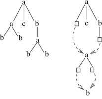
Figure 12: Left, a data tree, and right, a DAG representation of it.

We establish:

Theorem 3.

Let $P$ be an 1.0 program. Then the following problem is solvable in exponential, i.e., $2^{n^{O(1)}}$ time:

Input:

a data tree $\mathbf{t}$

Output:

a DAG representation of the final result tree of applying $P$ to $\mathbf{t}$, or a message signaling non-termination if $P$ does not terminate on $\mathbf{t}$.

Proof.

We will generate a DAG representation $\mathcal{G}$ by applying modified versions of the semantic rules from Section 5. We initialise $\mathcal{G}$ with all the subtrees of $\mathbf{t}$. These trees have no pointers. Each tree that will be added to $\mathcal{G}$ will be a configuration, which still has to be developed further into a final data tree with pointers, using the same modified rules. Because we will have to point to the newly added configurations later, we identify each added configuration by a pair $(\mathit{name},C)$ where $\mathit{name}$ is the name of a template rule in $P$ and $C$ is a context. In the description below, whenever we say that we “add” a configuration to $\mathcal{G}$, identified by some pair $(\mathit{name},C)$, we really mean that we add it unless a configuration identified by that same pair already exists in $\mathcal{G}$.

The modifications are now the following.

1. When executing an apply-statement, we do not directly insert copies of the templates belonging to the rules that must be applied (the $\gamma_{i}$’s in Figure 5). Rather, we add, for $i=1,\dots,k$, the configuration $\gamma_{i}^{\prime}$ to $\mathcal{G}$, where $\gamma_{i}\mathrel{\stackrel{{\scriptstyle\mathsf{if}}}{{\Rightarrow}}{}^{!}}\gamma_{i}^{\prime}$. We identify $\gamma_{i}^{\prime}$ by the pair $(\mathit{name}_{i},C_{i})$, with $\mathit{name}_{i}$ the name of the rule $\gamma_{i}$ comes from, and $C_{i}=(\mathbf{S},\mathbf{E},(\mathbf{n}_{i},i,k))$ using the notation of Figure 5. Moreover, in place of the apply-statement we insert a sequence of $k$ pointer nodes pointing to $(\mathit{name}_{1},C_{1})$, …, $(\mathit{name}_{k},C_{k})$, respectively.

2. When executing a call-statement call $\mathit{name}$ under context $C$, we again do not insert $\gamma_{1}$ (compare Figure 5), but add the configuration $\gamma_{1}^{\prime}$ to $\mathcal{G}$, where $\gamma_{1}\mathrel{\stackrel{{\scriptstyle\mathsf{if}}}{{\Rightarrow}}{}^{!}}\gamma_{1}^{\prime}$, and identify it by the pair $(\mathit{name},C)$. We then replace the statement by a pointer node pointing to that pair.

3. By making template rules from the bodies of all foreach-statements in $P$, we may assume without loss of generality that the body of every foreach-statement is a single call-statement. A foreach-statement is then processed analogously to apply- and call-statements.

4. As we did with foreach-statements, we may assume that the body of each tree-statement is a single call-statement. When executing a tree-statement, we may assume that the call-statement has already been turned into a pointer to some pair $(\mathit{name}_{0},C_{0})$. We then assign that pair directly to $y$ in the new context $C^{\prime}$ (compare Figure 6); we no longer apply $\mathit{maketree}$.

   So, in the modified kind of store we use, we assign name–context pairs, rather than fully specified temporary trees, to tree variables.

5. Correspondingly, when executing a statement tcopy $y$, we now directly turn it into a pointer to the pair assigned to $y$.

6. Finally, when executing a vcopy-statement, we do not insert the whole forest generated by $(\mathbf{n}_{1},\dots,\mathbf{n}_{k})$ in the configuration (compare Figure 8), but merely insert a sequence of $k$ pointers to the input subtrees rooted at $\mathbf{n}_{1}$, …, $\mathbf{n}_{k}$, respectively.

We initiate the generation of $\mathcal{G}$ by starting with the initial configuration as always. Processing that configuration will add the first tree to $\mathcal{G}$, which serves as the root tree of the DAG representation. When all trees in $\mathcal{G}$ have been fully developed into data trees with pointer nodes, the algorithm terminates. In case $P$ does not terminate on $\mathbf{t}$, however, that will never happen, and we need a way to detect nontermination.

Thereto, recall that every context consists of an environment $\mathbf{E}$ and a context triple $c$ on the one hand, and a store $\mathbf{S}$ on the other hand. Since all $\mathcal{X}$-expressions used are input-only, and thus oblivious to the store-part of a context (except for the input tree, which does not change), we are in an infinite loop from the moment that there is a cycle in $\mathcal{G}$’s pointer graph where we ignore the store-part of the contexts. More precisely, this happens when from a pointer node in a tree identified by $(\mathit{name},C_{1})$ we can follow pointers and reach a pointer to a pair $(\mathit{name},C_{2})$ with the same $\mathit{name}$ and where $C_{1}$ and $C_{2}$ are equal in their $(\mathbf{E},c)$-parts. As soon as we detect such a cycle, we terminate the algorithm and signal nontermination. Note that thus the algorithm always terminates. Indeed, since only input-only $\mathcal{X}$-expressions are used, all contexts that appear in the computation are input-only, and there are only a finite number of possible $(\mathbf{E},c)$-parts of input-only configuration over a fixed input tree.

Let us analyse the complexity of this algorithm. Since all $\mathcal{X}$-expressions used are polynomial, there is a natural number $K$ such that each value that appears in a context is at most $n^{K}$ long, where $n$ equals the number of nodes in $\mathbf{t}$. Each element of such a length-$n^{K}$ sequence is a node or a counter over $\mathbf{t}$, so there are at most $(2n)^{n^{K}}$ different values. There are a constant $c_{1}$ number of different value variables in $P$, so there are at most $((2n)^{n^{K}})^{c_{1}}$ different environments. Likewise, the number of different context triples is $(2n)^{3}$, so, ignoring the stores, there are in total at most $(2n)^{3}\cdot(2n)^{c_{1}n^{K}}\leqslant 2^{n^{K^{\prime}}}$ different contexts, for some natural number $K^{\prime}\geqslant K$. With a constant $c_{2}$ number of different template names in $P$, we get a maximal number of $c_{2}2^{n^{K^{\prime}}}$ different configurations that can be added to $\mathcal{G}$ before the algorithm will surely terminate.

It remains to see how long it takes to fully rewrite each of those configurations into a data tree with pointers. A configuration initially consists of at most a constant $c_{3}$ number of statements. The evaluation of $\mathcal{X}$-expressions, which are polynomial, takes at most $c_{3}n^{K}$ time in total. Processing an apply- or a foreach-statement takes at most $c_{3}n^{K}$ modifications to the configuration and to $\mathcal{G}$; for the other statements this takes at most $c_{3}$ such operations. Each such operation, however, involves the handling of contexts, whose stores can become quite large if treated naively. Indeed, tree-statements assign a context to a tree variable, yielding a new context which may then again be assigned to a tree variable, and so on. To keep this under control, we do not copy the contexts literally, but number them consecutively in the order they are introduced in $\mathcal{G}$. A map data structure keeps track of this numbering. The stores then consist of an at most constant $c_{4}$ number of assignments of pairs (name, context number) to tree variables. As there are at most $2^{n^{K^{\prime}}}$ different contexts, each number is at most $n^{K^{\prime}}$ bits long. Looking up whether a given context is already in $\mathcal{G}$, and if so, finding its number, takes $O(\log 2^{n^{K^{\prime}}})=O(n^{K^{\prime}})$ time using a suitable map data structure.

We conclude that the processing of $\mathcal{G}$ takes a total time of $c_{2}2^{n^{K^{\prime}}}\cdot O(n^{K^{\prime}})=2^{n^{O(1)}}$, as had to be proven. ∎

A legitimate question is whether the complexity bound given by Theorem 3 can still be improved. In this respect we can show that, even within the limits of real XSLT 1.0, any linear-space turing machine can be simulated by a 1.0 program. Note that some PSPACE-complete problems, such as QBF-SAT [21], are solvable in linear space. This shows that the time complexity upper bound of Theorem 3 cannot be improved without showing that PSPACE is properly included in EXPTIME (a famous open problem).

The simulation gets as input a flat tree representing an input string, and uses the $n$ child nodes to simulate the $n$ tape cells. For each letter a of the tape alphabet, a value variable $\mathit{cell}_{\text{{a}}}$ holds the nodes representing the tape cells that have an a. A value variable $\it head$ holds the node representing the cell seen by the machine’s head. The machine’s state is kept by additional value variables ${\it state}_{q}$ for each state $q$, such that ${\it state}_{q}$ is nonempty iff the machine is in state $q$. Writing a letter in a cell, moving the head left or right, or changing state, are accomplished by easy updates on the value-variables, which can be expressed by real XPath 1.0 expressions. Choosing the right transition is done by a big if-then-else statement. Successive transitions are performed by recursively applying the simulating template rule until a halting state is reached.

Remark 7.1.

A final remark is that our results imply that XSLT 1.0 is not closed under composition. Indeed, building up a tree of doubly exponential size (as we already remarked is possible in XSLT 1.0), followed by the building up of a tree of exponential size, amounts to building up a tree of triply exponential size. If that would be possible by a single program, then a DAG representation of a triply exponentially large tree would be computable in singly exponential time. It is well known, however, that a DAG representation cannot be more than singly exponentially smaller than the tree it represents. Closure under composition is another sharp contrast between XSLT 1.0 and 2.0, as the latter is indeed closed under composition as already noted in the proof of Theorem 2.

8 Conclusions

W3C recommendations such as the XSLT specifications are no Holy scriptures. Theoretical scrutinising of W3C work, which is what we have done here, can help in better understanding the possibilities and limitations of various newly proposed programming languages related to the Web, eventually leading to better proposals.

A formalisation of the full XSLT 2.0 language, with all the dirty details both concerning the language itself as concerning the XPath 2.0 data model, is probably something that should be done. We believe our work gives a clear direction how this could be done.

Note also that XSLT contains a lot of redundancies. For example, foreach-statements are eliminable, as are call-statements, and the match attribute of template rules. A formalisation such as ours can provide a rigorous foundation to prove such redundancies, or to prove correct various processing strategies or optimisation techniques XSLT implementations may use.

A formal tree transformation model denoted by TL, in part inspired by XSLT, but still omitting many of its features, has already been studied by Maneth and his collaborators [9, 19]. The TL model can be compiled into the earlier formalism of “macro tree transducers” [12, 23]. It is certainly an interesting topic for further research to similarly translate our XSLT formalisation (even partially) into macro tree transducers, so that techniques already developed for these transducers can be applied. For example, under regular expression types [15] (known much earlier under the name of “recognisable tree languages”), exact automated typechecking is possible for compositions of macro tree transducers, using the method of “inverse type inference” [20]. This method has various other applications, such as deciding termination on all possible inputs [19]. Being able to apply this method to our XSLT 1.0 formalism would improve the analysis techniques of Dong and Bailey [11], which are not complete.

Appendix A Real XSLT programs

A.1 Figure 10 in real XSLT

<xsl:transform
  xmlns:xsl="http://www.w3.org/1999/XSL/Transform"
  version="1.0">

  <xsl:template name="tree2string" match="//*">
    <a/>
    <lbrace/>
    <xsl:apply-templates select="child::*"/>
    <rbrace/>
  </xsl:template>

</xsl:transform>

A.2 Figure 11 in real XSLT

<xsl:transform
  xmlns:xsl="http://www.w3.org/1999/XSL/Transform"
  version="1.0">

<xsl:template match="/doc">
  <xsl:apply-templates select="child::*[1]"/>
</xsl:template>

<xsl:template name="string2tree" match="/doc//*">
  <a>
    <xsl:apply-templates select="following-sibling::*[1]" mode="dochildren"/>
  </a>
  <xsl:call-template name="searchnextsibling">
    <xsl:with-param name="counter" select="1"/>
  </xsl:call-template>
</xsl:template>

<xsl:template match="//*" mode="dochildren">
  <xsl:if test="name()=’lbrace’">
    <xsl:apply-templates select="following-sibling::*[1]" mode="dochildren"/>
  </xsl:if>
  <xsl:if test="name()=’a’">
    <xsl:call-template name="string2tree"/>
  </xsl:if>
</xsl:template>

<xsl:template name="searchnextsibling" match="//*" mode="search">
  <xsl:param name="counter"/>
  <xsl:if test="name()=’lbrace’">
    <xsl:apply-templates select="following-sibling::*[1]" mode="search">
      <xsl:with-param name="counter" select="$counter + 1"/>
    </xsl:apply-templates>
  </xsl:if>
  <xsl:if test="name()=’a’">
    <xsl:apply-templates select="following-sibling::*[1]" mode="search">
      <xsl:with-param name="counter" select="$counter"/>
    </xsl:apply-templates>
  </xsl:if>
  <xsl:if test="name()=’rbrace’">
    <xsl:if test="$counter=2">
      <xsl:apply-templates select="following-sibling::*[1]" mode="dochildren"/>
    </xsl:if>
    <xsl:if test="$counter>2">
      <xsl:apply-templates select="following-sibling::*[1]" mode="search">
        <xsl:with-param name="counter" select="$counter - 1"/>
      </xsl:apply-templates>
    </xsl:if>
  </xsl:if>
</xsl:template>

</xsl:transform>

References

- [1] XML path language (XPath) version 1.0. W3C Recommendation, November 1999.
- [2] XSL transformations (XSLT) version 1.0. W3C Recommendation, November 1999.
- [3] XSLT requirements version 2.0. W3C Working Draft, February 2001.
- [4] XML schema. W3C Recommendation, October 2004.
- [5] XML path language (XPath) version 2.0. W3C Working Draft, April 2005.
- [6] XQuery 1.0 and XPath 2.0 data model. W3C Working Draft, April 2005.
- [7] XQuery 1.0 and XPath 2.0 formal semantics. W3C Working Draft, June 2005.
- [8] XSL transformations (XSLT) version 2.0. W3C Working Draft, April 2005.
- [9] G.J. Bex, S. Maneth, and F. Neven. A formal model for an expressive fragment of XSLT. Information Systems, 27(1):21–39, 2002.
- [10] P. Buneman, M. Grohe, and C. Koch. Path queries on compressed XML. In J.C. Freytag, P.C. Lockemann, et al., editors, Proceedings 29th International Conference on Very Large Data Bases, pages 141–152. Morgan Kaufmann, 2003.
- [11] C. Dong and J. Bailey. Static analysis of XSLT programs. In K.D. Schewe and H.E. Williams, editors, Database technologies—Proceedings ADC 2004, pages 151–160. Australian Computer Society, 2004.
- [12] J. Engelfriet and H. Vogler. Macro tree transducers. Journal of Computer and System Sciences, 31(1):71–146, 1985.
- [13] G. Gottlob, C. Koch, and R. Pichler. XPath processing in a nutshell. SIGMOD Record, 32(2):21–27, 2003.
- [14] J. Hidders, J. Paredaens, R. Vercammen, et al. A light but formal introduction to XQuery. In Z. Bellahsène, T. Milo, M. Rys, et al., editors, Database and XML Technologies—Proceedings XSym, volume 3186 of Lecture Notes in Computer Science, pages 5–20. Springer, 2004.
- [15] H. Hosoya and B.C. Pierce. XDuce: A statically typed XML processing language. ACM Transactions on Internet Technology, 3(2):117–148, 2003.
- [16] M. Kay. SAXON: The XSLT and XQuery processor. http://saxon.sourceforge.net.
- [17] M. Kay. XSLT 2.0 Programmer’s Reference. Wrox, 3rd edition, 2004.
- [18] S. Maneth. The complexity of compositions of deterministic tree transducers. In M. Agrawal and A. Seth, editors, FST TCS 2002 Proceedings, volume 2556 of Lecture Notes in Computer Science, pages 265–276. Springer, 2002.
- [19] S. Maneth, A. Berlea, T. Perst, and H. Seidl. XML type checking with macro tree transducers. In Proceedings 24th ACM Symposium on Principles of Database Systems, pages 283–294. ACM Press, 2005.
- [20] T. Milo, D. Suciu, and V. Vianu. Typechecking for XML transformers. Journal of Computer and System Sciences, 66(1):66–97, 2003.
- [21] C.H. Papadimitriou. Computational Complexity. Addison-Wesley, 1994.
- [22] M.S. Paterson and M.N. Wegman. Linear unification. Journal of Computer and System Sciences, 16(2):158–167, 1978.
- [23] T. Perst and H. Seidl. Macro forest transducers. Information Processing Letters, 89(3):141–149, 2004.
- [24] B.K. Rosen. Tree-manipulating systems and Church-Rosser theorems. Journal of the ACM, 20(1):160–187, 1973.
- [25] J. Siméon and P. Wadler. The essence of XML. In Proceedings 30th ACM Symposium on Principles of Programming Languages, pages 1–13. ACM Press, 2003.
- [26] Terese. Term Rewriting Systems. Cambridge University Press, 2003.
- [27] P. Wadler. A formal semantics of patterns in XSLT and XPath. Markup Languages: Theory and Practice, 2(2):183–202, 2000.