On the Second-Order Statistics of the Instantaneous Mutual Information in Rayleigh Fading Channels

Abstract

In this paper, the second-order statistics of the instantaneous mutual information are studied, in time-varying Rayleigh fading channels, assuming general non-isotropic scattering environments. Specifically, first the autocorrelation function, correlation coefficient, level crossing rate, and the average outage duration of the instantaneous mutual information are investigated in single-input single-output (SISO) systems. Closed-form exact expressions are derived, as well as accurate approximations in low- and high-SNR regimes. Then, the results are extended to multiple-input single-output and single-input multiple-output systems, as well as multiple-input multiple-output systems with orthogonal space-time block code transmission. Monte Carlo simulations are provided to verify the accuracy of the analytical results. The results shed more light on the dynamic behavior of the instantaneous mutual information in mobile fading channels.

I Introduction

The increasing demand for wireless communication over time-varying channels has motivated further investigation of the channel dynamics and its statistical behavior. There are numerous studies on the temporal second-order characteristics of a variety of terrestrial [1, 2, 3, 4] and satellite channels [5], such as the correlation function, level crossing rate (LCR), and average fade duration.

For such important quantity as the instantaneous mutual information (IMI), however, only the mean value, which is the ergodic capacity, has received much attention as well as the outage probability[6, 7]. Clearly, ergodic capacity and outage probability do not show the dynamic temporal behavior of IMI in time-varying fading channels. For example, the outage probability of a fading channel gives the probability of IMI to be smaller than a particular data rate[6]. Nevertheless, it does not show how long, on average, IMI stays below that rate. To the best of our knowledge, only some simulation results regarding such second-order statistics are given in[8], without analytical results, and in [9], lower and upper bounds on the correlation coefficient in the high signal-to-noise ratio (SNR) regime, as well as some approximations, are derived without exact results.

In this paper, several second-order statistics of IMI are studied in time-varying Rayleigh flat fading channels, considering a general non-isotropic scattering propagation environment. Closed-form expressions and simple approximations are derived for the autocorrelation function (ACF), correlation coefficient, LCR and the average outage duration (AOD) of IMI. A variety of channels are considered such as multiple-input single-output (MISO), single-input multiple-output (SIMO), multiple-input multiple-output with orthogonal space-time block code (OSTBC) transmission, and MIMO in the low-SNR regime. Monte Carlo simulations are provided to verify the accuracy of our closed-form expressions and approximate results.

Notation: ^† is reserved for matrix Hermitian, ^⋆ for complex conjugate, $\operatorname{tr}[\cdot]$ for the trace of a square matrix, $\jmath$ for $\sqrt{-1}$, $\mathbb{E}[\cdot]$ for mathematical expectation, $\mathbf{I}_{m}$ for the $m\times m$ identity matrix, $\ln(\cdot)$ for the natural logarithm, $\log_{2}(\cdot)$ for the base-2 logarithm, $\mathcal{O}(\cdot)$ for the order, $\|\cdot\|_{F}$ for the Frobenius norm, $f^{2}(x)$ for $\left[f(x)\right]^{2}$, and $\max_{a\leq x\leq b}f(x)$ for the maximum of $f(x)$ over the range $a\leq x\leq b$.

The rest of this paper is organized as follows. Sec. II introduces the IMI random process in a single-input single-output (SISO) system, whereas the channel and angle-of-arrival (AoA) models are described in Appendix A. Sec. III is devoted to the derivation of ACF and the correlation coefficient of IMI in SISO channels, as well as their low- and high-SNR approximations. The LCR and AOD of SISO IMI are derived in Sec. IV. Extension of the SISO results systems with multiple antennas are discussed in Sec. V. Numerical results are presented in Sec. VI, and concluding remarks are given in Sec. VII.

II The SISO IMI

Similar to [6], we consider a piecewise constant approximation for the continuous-time SISO fading channel coefficient $h(t)$, represented by $\left\{h(lT_{\!s})\right\}_{l=1}^{L}$, where $T_{\!s}$ is the symbol duration and $L$ is the number of samples. In the presence of additive white Gaussian noise, if perfect channel state information $\left\{h(lT_{\!s})\right\}_{l=1}^{L}$ is available at the receiver only, the ergodic channel capacity is given by[6, 7]

$$C=\mathbb{E}\left[\log_{2}\left(1+\eta\alpha_{l}^{2}\right)\right],$$ (1)

bps/Hz, where $\eta$ is the average SNR at the receiver side, $\alpha_{l}$ is the envelop of $h(lT_{\!s})$, i.e., $\alpha_{l}=|h(lT_{\!s})|,\forall l$. We choose $\mathbb{E}[\alpha_{l}^{2}]=1$, i.e., the channel has unit power.

In the above equation, at any given time index $l$, $\log_{2}(1+\eta\alpha^{2}_{l})$ is a random variable as it depends on the fading parameter $\alpha_{l}$[6]. Therefore

$$\mathcal{I}_{l}=\log_{2}\left(1+\eta\alpha^{2}_{l}\right),\quad l=1,2,\cdots,$$ (2)

is a discrete-time random process with the ergodic capacity as its mean. We study the second-order statistics of $\{\mathcal{I}_{l}\}_{l=1}^{\infty}$, such as autocorrelation, correlation coefficient, LCR and AOD, in the following sections.

III ACF and Correlation Coefficient
of the SISO IMI

In this section, first we concentrate on the ACF of IMI, define in (2). The ACF is defined by

$$r_{\mathcal{I}}(i) \!=\!\mathbb{E}[\mathcal{I}_{l}\mathcal{I}_{l-i}],$$ (3)

$$\!=\!(\log_{2}e)^{2}\mathbb{E}\!\left[\ln(1\!+\!\eta x_{1})\!\ln(1\!+\!\eta x_{2})\right],$$ (4)

where $x_{1}=\alpha^{2}_{l}$, $x_{2}=\alpha^{2}_{l-i}$, and $x_{1}$ and $x_{2}$ have a joint Chi-square probability density function (PDF) with 2 degrees of freedom[6, (3.2)][10, pp. 163, (8-103)]

$$p(x_{1},x_{2})=\lambda_{i}e^{-\lambda_{i}(x_{1}+x_{2})}I_{0}\!\left(2\lambda_{i}\varrho_{i}\sqrt{x_{1}x_{2}}\right),$$ (5)

where $\lambda_{i}=\frac{1}{1-\varrho_{i}^{2}}$, $\varrho_{i}=|\rho_{h}(iT_{\!s})|<1$, $i\neq 0$, $\rho_{h}(\tau)=\mathbb{E}[h(t)h^{\star}(t-\tau)]$ is the correlation coefficient of the Rayleigh fading channel, and $I_{k}(z)=\frac{1}{\pi}\int_{0}^{\pi}e^{z\cos\theta}\cos(k\theta)\mathrm{d}\theta$ is the $k^{\text{th}}$ order modified Bessel function of the first kind. A closed-form expression for $\rho_{h}(\tau)$ in non-isotropic scattering environments is given in the Appendix A.

Combining (4) and (5), with the following Taylor series [11, pp. 971, 8.447.1]

$$I_{0}(t)=\sum_{k=0}^{\infty}\frac{t^{2k}}{(k!)^{2}2^{2k}},$$ (6)

simplifies (4) to the following exact infinite-summation closed-form representation

$$\begin{split}\frac{r_{\mathcal{I}}(i)}{(\log_{2}e)^{2}}\!&=\!\lambda_{i}\!\sum_{k=0}^{\infty}\!\frac{(\lambda_{i}\varrho_{i})^{2k}}{(k!)^{2}}\!\left[\int_{0}^{\infty}\!\!\!\!x^{k}\ln(1\!+\!\eta x)e^{-\lambda_{i}x}\mathrm{d}x\right]^{2}\\ \!&=\!\!\frac{1}{\lambda_{i}}\sum_{k=0}^{\infty}\!\left[\frac{\varrho_{i}^{k}}{k!}G_{2,3}^{3,1}\!\!\left(\!\frac{\lambda_{i}}{\eta}\!\left|\!\!\begin{array}[]{c}0,1\\ 0,0,k\!+\!1\end{array}\right.\!\!\!\!\right)\!\!\right]^{\!2}\!\!\!\!,\end{split}$$ (7)

where $G$ is Meijer’s $G$ function[11, pp. 1096, 9.301] and the normalized ACF is given by

$$\tilde{r}_{\mathcal{I}}(i)=\frac{r_{\mathcal{I}}(i)}{\mathbb{E}[\mathcal{I}_{l}^{2}]}=\frac{{\displaystyle\frac{1}{\lambda_{i}}\sum_{k=0}^{\infty}}\!\left[\frac{\varrho_{i}^{k}}{k!}G_{2,3}^{3,1}\!\!\left(\!\frac{\lambda_{i}}{\eta}\!\left|\!\!\begin{array}[]{c}0,1\\ 0,0,k\!+\!1\end{array}\right.\!\!\!\!\right)\!\right]^{\!2}}{2e^{\frac{1}{\eta}}G_{2,3}^{3,0}\!\!\left(\frac{1}{\eta}\!\left|\!\!\begin{array}[]{c}1,1\\ 0,0,0\end{array}\right.\!\!\right)}.$$ (8)

After some algebraic manipulations, we obtain the correlation coefficient as

$$\rho_{\mathcal{I}}(i) =\frac{r_{\mathcal{I}}(i)-\{\mathbb{E}[\mathcal{I}_{l}]\}^{2}}{\mathbb{E}[\mathcal{I}_{l}^{2}]-\{\mathbb{E}[\mathcal{I}_{l}]\}^{2}},$$ (9)

$$=\frac{{\displaystyle\frac{1}{\lambda_{i}}\sum_{k=0}^{\infty}}\!\left[\frac{\varrho_{i}^{k}}{k!}G_{2,3}^{3,1}\!\!\left(\!\frac{\lambda_{i}}{\eta}\!\left|\!\!\begin{array}[]{c}0,1\\ 0,0,k\!+\!1\end{array}\right.\!\!\!\!\right)\!\right]^{\!2}\!\!-\!e^{\frac{2}{\eta}}\Gamma^{2}\!\left(0,\frac{1}{\eta}\right)}{2e^{\frac{1}{\eta}}G_{2,3}^{3,0}\!\!\left(\frac{1}{\eta}\!\left|\!\!\begin{array}[]{c}1,1\\ 0,0,0\end{array}\right.\!\!\right)-e^{\frac{2}{\eta}}\Gamma^{2}\!\left(0,\frac{1}{\eta}\right)},$$ (14)

where $\Gamma(a,z)=\int_{z}^{\infty}t^{a-1}e^{-t}\mathrm{d}t$[11, pp. 949, 8.350.2] is the upper incomplete gamma function. The derivation of (7), (8) and (14) are given in Appendix B.

In general, it seems difficult to further simplify (8) and (14). However, we note that the integral $\Xi(k,\eta,\lambda_{i})=\int_{0}^{\infty}x^{k}e^{-\lambda_{i}x}\ln(1+\eta x)\mathrm{d}x$, $k\geq 0$, can be approximated by

$$\Xi(k,\eta,\lambda_{i})\approx\begin{cases}\int_{0}^{\infty}\eta x^{k+1}e^{-\lambda_{i}x}\mathrm{d}x,&\eta\rightarrow 0,\\ \int_{0}^{\infty}x^{k}e^{-\lambda_{i}x}\ln(\eta x)\mathrm{d}x,&\eta\rightarrow\infty,\end{cases}$$ (15)

using $\ln(1+\eta x)\approx\eta x$, $\eta\rightarrow 0$, and $\ln(1+\eta x)\approx\ln\left(\eta x\right)$, $\eta\rightarrow\infty$, respectively.

In the following two subsections, we will use (7) and (15) to derive asymptotic closed-form expressions for $r_{\mathcal{I}}(i)$ in the low- and high-SNR regimes.

III-A Low-SNR Regime

If $\eta\rightarrow 0$, based on (7) and (15), we have

$$\frac{r_{\mathcal{I}}(i)}{(\log_{2}e)^{2}}\!\approx\!\lambda_{i}\!\sum_{k=0}^{\infty}\frac{\Xi_{L}^{2}(k,\eta,\lambda_{i})}{(\lambda_{i}\varrho_{i})^{-2k}(k!)^{2}},$$ (16)

where $\Xi_{L}(k,\eta,\lambda_{i})$ is defined as $\eta\!\int_{0}^{\infty}\!\!x^{k+1}e^{-\lambda_{i}x}\mathrm{d}x$ and given by[11, pp. 364, 3.381.4]

$$\Xi_{L}(k,\eta,\lambda_{i})=\eta\frac{(k+1)!}{\lambda_{i}^{k+2}}.$$ (17)

By replacing $\Xi_{L}(k,\eta,\lambda_{i})$ in (16) with (17), we obtain

$$\begin{split}\frac{r_{\mathcal{I}}(i)}{(\log_{2}e)^{2}}\!&\approx\!\lambda_{i}\!\sum_{k=0}^{\infty}\!\frac{(\lambda_{i}\varrho_{i})^{2k}}{(k!)^{2}}\!\left[\!\eta\frac{(k+1)!}{\lambda_{i}^{k+2}}\right]^{2},\\ \!&=\!\!\frac{\eta^{2}}{\lambda_{i}^{3}\varrho_{i}^{2}}\!\sum_{k=1}^{\infty}\!k^{2}\varrho_{i}^{2k}.\end{split}$$ (18)

Since $\varrho_{i}<1$, we have

$$\sum_{k=1}^{\infty}\!k^{2}\varrho_{i}^{2k}=\left.t\frac{\partial}{\partial t}\left[t\left(\frac{\partial}{\partial t}\sum_{k=1}^{\infty}t^{k}\right)\right]\right|_{t=\varrho_{i}^{2}}\!\!\!\!=\lambda_{i}^{3}\varrho_{i}^{2}(1+\varrho_{i}^{2}),$$ (19)

which simplifies (18) to

$$r_{\mathcal{I}}(i)\approx(\log_{2}e)^{2}\eta^{2}(1+\varrho_{i}^{2}).$$ (20)

After normalization by $\mathbb{E}[\mathcal{I}_{l}^{2}]=r_{\mathcal{I}}(0)\approx 2(\log_{2}e)^{2}\eta^{2}$, we obtain

$$\tilde{r}_{\mathcal{I}}(i)\approx\frac{1+\varrho_{i}^{2}}{2}.$$ (21)

Moreover, the correlation coefficient is given by

$$\rho_{\mathcal{I}}(i)\!\approx\!\frac{r_{\mathcal{I}}(i)\!-\!\{\!\left(\log_{2}\!e\!\right)\!\mathbb{E}[\eta x]\!\}^{2}}{\mathbb{E}[\mathcal{I}_{l}^{2}]\!-\!\{\!\left(\log_{2}\!e\!\right)\!\mathbb{E}[\eta x]\!\}^{2}}\!=\!\frac{\eta^{2}(1\!+\!\varrho_{i}^{2})\!-\!\eta^{2}}{2\eta^{2}\!-\!\eta^{2}}\!=\!\varrho_{i}^{2},$$ (22)

where we use $\mathbb{E}[x]=\mathbb{E}[\alpha_{l}^{2}]=1$, due to the unit-power Rayleigh fading assumption.

With isotropic scattering, we have $\rho_{h}(\tau)=J_{0}(2\pi f_{m}\tau)$, the Clarke’s correlation[1], where $f_{m}$ is the maximum Doppler frequency, and $J_{0}(x)=\frac{1}{\pi}\int_{0}^{\pi}e^{\jmath x\cos\theta}\mathrm{d}\theta$ is the zero-order Bessel function of the first kind. This simplifies (22) to $J_{0}^{2}(2\pi f_{m}iT_{\!s})$ with $\tau=iT_{\!s}$.

III-B High-SNR Regime

If $\eta\rightarrow\infty$, based on (7) and (15), we get

$$\frac{r_{\mathcal{I}}(i)}{(\log_{2}e)^{2}}\!\approx\!\lambda_{i}\!\sum_{k=0}^{\infty}\frac{\Xi_{H}^{2}(k,\eta,\lambda_{i})}{(\lambda_{i}\varrho_{i})^{-2k}(k!)^{2}},$$ (23)

where $\Xi_{H}(k,\eta,\lambda_{i})$ is defined as $\int_{0}^{\infty}\!\!x^{k}(\ln\eta+\ln x)e^{-\lambda_{i}x}\mathrm{d}x$. Using 4.352.2 [11, pp. 604] and (17), we obtain

$$\Xi_{H}(k,\eta,\lambda_{i})=\frac{k!}{\lambda_{i}^{k+1}}\left(\ln\frac{\eta}{\lambda_{i}\gamma}+{H}_{\!k}\right),$$ (24)

where $\gamma=1.781072\cdots$ is the Euler-Mascheroni constant [11, pp. xxx], ${H}_{\!k}$ is the $k^{\text{th}}$ harmonic number[12, pp. 29, (2.13)], defined by ${H}_{\!k}=\sum_{j=1}^{k}\frac{1}{j}$ for $k\geq 1$, and ${H}_{0}=0$. After lengthy algebraic calculations, finally the normalized ACF in the high-SNR regime is shown to be

$$\tilde{r}_{\mathcal{I}}(i)\approx\frac{\operatorname{Li}_{2}\!\left(\varrho_{i}^{2}\right)+\ln^{2}\!\frac{\eta}{\gamma}}{\frac{\pi^{2}}{6}+\ln^{2}\!\frac{\eta}{\gamma}},$$ (25)

where $\operatorname{Li}_{2}(x)$ is the dilogarithm function, defined as $\operatorname{Li}_{2}(x)=\sum_{k=1}^{\infty}\frac{x^{k}}{k^{2}},|x|\leq 1$. The correlation coefficient is given by

$$\rho_{\mathcal{I}}(i)\approx\frac{6\operatorname{Li}_{2}\!\left(\varrho_{i}^{2}\right)}{\pi^{2}}.$$ (26)

Derivation of (25) and (26) are given in Appendix C. With isotropic scattering, (26) reduces to

$$\rho_{\mathcal{I}}(i)\approx\frac{6\operatorname{Li}_{2}\!\!\left[J_{0}^{2}\!\left(2\pi f_{m}iT_{\!s}\right)\right]}{\pi^{2}}.$$ (27)

IV LCR and AOD of SISO IMI

IV-A The LCR of SISO IMI

Similar to the calculation of zero crossing rate in discrete time[13, Ch. 4], we define the binary sequence $\left\{X_{l}\right\}_{l=1}^{L}$, based on the IMI sequence $\left\{\mathcal{I}_{1}\right\}_{l=1}^{L}$, as

$$X_{l}=\begin{cases}1,&\text{if }\mathcal{I}_{l}\geq\mathcal{I}_{\text{th}},\\ 0,&\text{if }\mathcal{I}_{l}<\mathcal{I}_{\text{th}},\end{cases}$$ (28)

where $\mathcal{I}_{\text{th}}$ is a fixed threshold. The number of crossings of $\left\{\mathcal{I}_{1}\right\}_{l=1}^{L}$ with $\mathcal{I}_{\text{th}}$, within the time interval $T_{\!s}\leq t\leq LT_{\!s}$, denoted by $D_{\mathcal{I}_{\text{th}}}$, is defined in terms of $\{X_{l}\}_{l=1}^{L}$[13, (4.1)]

$$D_{\mathcal{I}_{\text{th}}}=\sum_{l=2}^{L}\left(X_{l}-X_{l-1}\right)^{2},$$ (29)

which includes both up- and down-crossings.

After some simple manipulations, the expected crossing rate at the level $\mathcal{I}_{\text{th}}$ can be written as

$$\frac{\mathbb{E}[D_{\mathcal{I}_{\text{th}}}]}{(L-1)T_{\!s}}=\frac{2P_{r}\{X_{l}=1\}-2P_{r}\{X_{l}=1,X_{l-1}=1\}}{T_{\!s}}.$$ (30)

Therefore the expected down crossing rate at the level $\mathcal{I}_{\text{th}}$, denoted by $N_{\mathcal{I}}(\mathcal{I}_{\text{th}})$, is given by

$$N_{\mathcal{I}}(\mathcal{I}_{\text{th}})=\frac{P_{r}\{X_{l}=1\}-P_{r}\{X_{l}=1,X_{l-1}=1\}}{T_{\!s}}.$$ (31)

To simplify the notation, we use $\phi$ for $P_{r}\{X_{l}=1\}$ and $\varphi(\varrho_{1})$ to denote $P_{r}\{X_{l}=1,X_{l-1}=1\}$, where $\varrho_{1}=|\rho_{h}(T_{\!s})|$, defined before. They can be calculated as follows

$$\phi=P_{r}\left\{\alpha^{2}_{l}\geq\frac{2^{\mathcal{I}_{\text{th}}}-1}{\eta}\right\}=\int_{\frac{2^{\mathcal{I}_{\text{th}}}-1}{\eta}}^{\infty}e^{-x}\mathrm{d}x=e^{-\frac{2^{\mathcal{I}_{\text{th}}}-1}{\eta}},$$ (32)

$$\begin{split}\varphi(\varrho_{1})&=P_{r}\left\{\alpha^{2}_{l}\geq\frac{2^{\mathcal{I}_{\text{th}}}-1}{\eta},\alpha^{2}_{l-1}\geq\frac{2^{\mathcal{I}_{\text{th}}}-1}{\eta}\right\},\\ &=\lambda_{1}\sum_{k=0}^{\infty}\frac{(\lambda_{1}\varrho_{1})^{2k}}{(k!)^{2}}\left[\int_{\frac{2^{\mathcal{I}_{\text{th}}}-1}{\eta}}^{\infty}x^{k}e^{-\lambda_{1}x}\mathrm{d}x\right]^{2},\\ &=\left(1-\varrho_{1}^{2}\right)\sum_{k=0}^{\infty}\left[\frac{\varrho_{1}^{k}}{k!}\Gamma\!\left(k+1,\frac{2^{\mathcal{I}_{\text{th}}}-1}{\eta\left(1-\varrho_{1}^{2}\right)}\right)\right]^{2}.\end{split}$$ (33)

By plugging (32) and (33) into (31), we obtain the expected crossing rate at the level $\mathcal{I}_{\text{th}}$ as

$$N_{\mathcal{I}}(\mathcal{I}_{\text{th}})\!\!=\!\!\frac{e^{-\frac{2^{\mathcal{I}_{\text{th}}}-1}{\eta}}}{T_{\!s}}-\frac{1-\varrho_{1}^{2}}{T_{\!s}}\!\sum_{k=0}^{\infty}\!\!\left[\!\frac{\varrho_{1}^{k}}{k!}\Gamma\!\!\left(\!k\!+\!1,\frac{2^{\mathcal{I}_{\text{th}}}\!-\!1}{\eta\!\left(1-\varrho_{1}^{2}\right)}\!\right)\!\!\right]^{2}\!\!\!\!.$$ (34)

IV-B The AOD of SISO IMI

Based on the relationship between $\mathcal{I}_{l}$ and $\alpha_{l}^{2}$ in (2), the cumulative distribution function (CDF) of $\mathcal{I}_{l}$ is obtained as

$$F_{\mathcal{I}}(\mathcal{\mathcal{I}_{\text{th}}})=P_{r}\left\{\alpha^{2}_{l}\leq\frac{2^{\mathcal{I}_{\text{th}}}-1}{\eta}\right\}=1-e^{-\frac{2^{\mathcal{I}_{\text{th}}}-1}{\eta}}.$$ (35)

The AOD of IMI, normalized by $T_{\!s}$, is therefore given by

$$\begin{split}\frac{\overline{t}_{\mathcal{I}}(\mathcal{I}_{\text{th}})}{T_{\!s}}&=\frac{F_{\mathcal{I}}(\mathcal{I}_{\text{th}})}{T_{\!s}N_{\mathcal{I}}(\mathcal{I}_{\text{th}})},\\ &=\frac{1-e^{-\frac{2^{\mathcal{I}_{\text{th}}}-1}{\eta}}}{e^{-\frac{2^{\mathcal{I}_{\text{th}}}-1}{\eta}}-\left(1-\varrho_{1}^{2}\right)\!\sum_{k=0}^{\infty}\!\!\left[\!\frac{\varrho_{1}^{k}}{k!}\Gamma\!\!\left(\!k\!+\!1,\frac{2^{\mathcal{I}_{\text{th}}}\!-\!1}{\eta\left(1-\varrho_{1}^{2}\right)}\!\right)\!\!\right]^{2}}.\end{split}$$ (36)

V Extension to Multiple Antenna Systems

For $N$-receiver (Rx) SIMO, $M$-transmitter (Tx) MISO, and $M$-Tx $N$-Rx OSTBC-based MIMO systems, we assume perfectly estimated, independent and identically distributed subchannels, with the same temporal correlation coefficient $\rho_{h}(\tau)$. Therefore the IMIs can be written as[14, 7][15, pp. 115, (7.4.43)]

$$\mathcal{I}^{SIMO}_{l} =\log_{2}\left[1+\eta\sum_{r=1}^{N}|h_{r}(lT_{\!s})|^{2}\right],$$ (37a)

$$\mathcal{I}^{MISO}_{l} =\log_{2}\left[1+\frac{\eta}{M}\sum_{t=1}^{M}|h_{t}(lT_{\!s})|^{2}\right],$$ (37b)

$$\mathcal{I}^{OSTBC}_{l} =\log_{2}\left[1+\frac{\eta}{M}\sum_{r=1}^{N}\sum_{t=1}^{M}|h_{r,t}(lT_{\!s})|^{2}\right],$$ (37c)

$$\tilde{r}_{\mathcal{I}}(i)=\frac{\frac{1}{2e^{\frac{M}{\eta}}\left(\frac{M\lambda_{i}}{\eta}\right)^{M\!N}}{\displaystyle\sum_{k=0}^{\infty}}\frac{\varrho_{i}^{2k}\left[G_{2,3}^{3,1}\!\left(\!\frac{M\lambda_{i}}{\eta}\!\left|\!\!\begin{array}[]{c}0,1\\ 0,0,k\!+\!M\!N\end{array}\right.\!\!\!\!\right)\right]^{2}}{k!(M\!N+k-1)!}}{{\displaystyle\sum_{j=0}^{M\!N-1}}{M\!N-1\choose j}(-1)^{M\!N-1-j}G_{3,4}^{4,0}\!\left(\!\frac{M}{\eta}\!\left|\begin{array}[]{c}-\!j,-\!j,-\!j\\ 0,-\!j\!-\!1,-\!j\!-\!1,-\!j\!-\!1\end{array}\right.\!\!\!\!\right)}.$$ (38)

$$\rho_{\mathcal{I}}(i)=\frac{\frac{(M\!N-1)!}{\lambda_{i}^{M\!N}}{\displaystyle\sum_{k=0}^{\infty}}\frac{\varrho_{i}^{2k}\left[G_{2,3}^{3,1}\!\left(\!\frac{M\lambda_{i}}{\eta}\!\left|\!\!\begin{array}[]{c}0,1\\ 0,0,k\!+\!M\!N\end{array}\right.\!\!\!\!\right)\right]^{2}}{k!(M\!N+k-1)!}-\left[G_{2,3}^{3,1}\!\left(\!\frac{M}{\eta}\!\left|\begin{array}[]{c}0,1\\ 0,0,M\!N\end{array}\right.\!\!\right)\right]^{2}}{2(M\!N\!-\!1)!e^{\frac{M}{\eta}}\left(\frac{M}{\eta}\right)^{M\!N}{\displaystyle\sum_{j=0}^{M\!N-1}}{M\!N-1\choose j}(-1)^{M\!N-1-j}G_{3,4}^{4,0}\!\left(\!\frac{M}{\eta}\!\left|\begin{array}[]{c}-\!j,-\!j,-\!j\\ 0,-\!j\!-\!1,-\!j\!-\!1,-\!j\!-\!1\end{array}\right.\!\!\!\!\right)-\left[G_{2,3}^{3,1}\!\left(\!\frac{M}{\eta}\!\left|\begin{array}[]{c}0,1\\ 0,0,M\!N\end{array}\right.\!\!\right)\right]^{2}}.$$ (39)

where $\eta$ is the expected SNR at each Rx antenna. Note that the SIMO and MISO systems in (37a) and (37b) are known as maximal ratio combiner (MRC) and maximal ratio transmitter (MRT), respectively[16].

It is easy to see (37c) includes (37a) and (37b) as special cases, by setting $M=1$ and $N=1$, respectively. Therefore, we only need to consider the OSTBC-based MIMO system.

At any time index $l$, $\sum_{r=1}^{N}\sum_{t=1}^{M}|h_{r,t}(lT_{\!s})|^{2}$ is a $\chi^{2}$ random variable with the $2M\!N$ degrees of freedom. We define $y_{1}=\sum_{r=1}^{N}\sum_{t=1}^{M}|h_{r,t}(lT_{\!s})|^{2}$ and $y_{2}=\sum_{r=1}^{N}\sum_{t=1}^{M}|h_{r,t}[(l-i)T_{\!s}]|^{2}$. The PDF of $y_{1}$ and the joint PDF of $y_{1}$ and $y_{2}$ are, respectively, given by[17, (2.32), (3.14)]

$$p(y_{1}) =\frac{y_{1}^{M\!N-1}e^{-y_{1}}}{(M\!N-1)!},$$ (40)

$$p(y_{1},y_{2}) =\frac{\lambda_{i}(y_{1}y_{2})^{\frac{M\!N-1}{2}}I_{M\!N-1}\!\left(2\lambda_{i}\varrho_{i}\sqrt{y_{1}y_{2}}\right)}{(M\!N-1)!\varrho_{i}^{M\!N-1}e^{\lambda_{i}(y_{1}+y_{2})}}.$$ (41)

According to the series representation of the modified Bessel function of the first kind[11, pp. 971, 8.445], we can rewrite (41) as

$$p(y_{1},y_{2})=\frac{\lambda_{i}^{M\!N}(y_{1}y_{2})^{M\!N-1}}{(M\!N-1)!e^{\lambda_{i}(y_{1}+y_{2})}}\sum_{k=0}^{\infty}\frac{(\lambda_{i}\varrho_{i})^{2k}(y_{1}y_{2})^{k}}{k!(M\!N+k-1)!}.$$ (42)

V-A ACF and Correlation Coefficient

By substituting (37c), (40) and (41) into (3), (8) and (9), after some manipulations, we obtained the normalized ACF and the correlation coefficient as shown in (38) and (39), respectively, whose derivations are given in Appendix D-A. Note that ${m\choose n}=\frac{m!}{(m-n)!n!}$, $m\geq n$, in (38) and (39).

V-A1 Low-SNR Regime

In Appendix D-B, the normalized ACF and the correlation coefficient are, respectively, expressed as

$$\tilde{r}_{\mathcal{I}}(i)\approx\frac{M\!N+\varrho_{i}^{2}}{M\!N+1},$$ (43)

and

$$\rho_{\mathcal{I}}(i)\approx\varrho_{i}^{2}.$$ (44)

As expected, (43) reduces to (21), when $M=N=1$. Interestingly, the correlation coefficient in the OSTBC-MIMO system is the same as that in the SISO system.

V-A2 High-SNR Regime

The normalized ACF is shown to be

$$\tilde{r}_{\mathcal{I}}(i)\approx\frac{\frac{(1-\varrho_{i}^{2})^{M\!N}R_{2}(\varrho_{i}^{2})}{(M\!N-1)!}+\left({H}_{\!M\!N-1}+\ln\frac{\eta}{M\gamma}\right)^{2}}{\left({H}_{\!M\!N-1}+\ln\frac{\eta}{M\gamma}\right)^{2}+\zeta(2,M\!N)}\\ -\frac{\left[{H}_{\!M\!N-1}-\ln(1-\varrho_{i}^{2})\right]^{2}}{\left({H}_{\!M\!N-1}+\ln\frac{\eta}{M\gamma}\right)^{2}+\zeta(2,M\!N)},$$ (45)

where $\zeta(z,q)=\sum_{k=0}^{\infty}\frac{1}{(q+k)^{z}}$ [11, pp. 1101, 9.521.1] and $R_{2}(\varrho_{i}^{2})$ is given in (84). Therefore, the correlation coefficient is

$$\rho_{\mathcal{I}}(i)\approx\frac{\frac{(1-\varrho_{i}^{2})^{M\!N}R_{2}(\varrho_{i}^{2})}{(M\!N-1)!}-\left[{H}_{\!M\!N-1}-\ln(1-\varrho_{i}^{2})\right]^{2}}{\zeta(2,M\!N)}.$$ (46)

Derivation of (45) and (46) can be found in Appendix D-C. We have checked that for $M=N=1$, (45) and (46) simplify to (25) and (26), respectively, using $R_{2}(\varrho_{i}^{2})=S_{2}(\varrho_{i}^{2})$ in (67c).

To obtain some insight, we consider a $2\times 2$ OSTBC-MIMO system in the high-SNR regime. For $M=N=2$, (81), (83) and (84) reduce to

$$R_{0}(\varrho_{i}^{2}) =\frac{6}{(1-\varrho_{i}^{2})^{4}},$$ (47a)

$$R_{1}(\varrho_{i}^{2}) =\frac{11-6\ln(1-\varrho_{i}^{2})}{(1-\varrho_{i}^{2})^{4}},$$ (47b)

$$R_{2}(\varrho_{i}^{2}) \!=\!\frac{6\ln^{2}(1\!-\!\varrho_{i}^{2})\!+\!6\operatorname{Li}_{2}\!\left(\varrho_{i}^{2}\right)}{(1-\varrho_{i}^{2})^{4}}\!+\!\frac{2\left(3\varrho_{i}^{4}\!+\!4\varrho_{i}^{2}\!-\!1\right)}{\varrho_{i}^{4}(1-\varrho_{i}^{2})^{4}}$$

$$\hskip 10.00002pt-\frac{\left(11\varrho_{i}^{6}+18\varrho_{i}^{4}-9\varrho_{i}^{2}+2\right)\ln(1-\varrho_{i}^{2})}{\varrho_{i}^{6}(1-\varrho_{i}^{2})^{4}}.$$ (47c)

To derive (47c) from (84), we need the integral representation of $\operatorname{Li}_{2}(t)$ as $\operatorname{Li}_{2}(t)=-\int_{0}^{t}\frac{\ln(1-z)}{z}\mathrm{d}z$, which can be derived from 0.241.4 in [11, pp. 12], by using $\int_{0}^{1}\frac{\ln(1-z)}{z}\mathrm{d}z=-\frac{\pi^{2}}{6}$[11, pp. 586, 4.291.2].

$$\frac{\overline{t}_{\mathcal{I}}(\mathcal{I}_{th})}{T_{\!s}}=\frac{\gamma\!\left(M\!N,\frac{2^{\mathcal{I}_{\text{th}}}-1}{\eta/M}\right)}{\Gamma\!\left(M\!N,\frac{2^{\mathcal{I}_{\text{th}}}-1}{\eta/M}\right)-\left(1-\varrho_{1}^{2}\right)^{M\!N}{\displaystyle\sum_{k=0}^{\infty}}\frac{\varrho_{1}^{2k}}{k!(M\!N+k-1)!}\Gamma^{2}\!\left(k+M\!N,\frac{M\left(2^{\mathcal{I}_{\text{th}}}-1\right)}{\eta\left(1-\varrho_{1}^{2}\right)}\right)}.$$ (48)

Using (47c), (45) and (46) reduce to, respectively,

$$\begin{split}\tilde{r}_{\mathcal{I}}(i)&\approx\frac{6+22\ln\frac{\eta}{2\gamma}+6\ln^{2}\frac{\eta}{2\gamma}+6\operatorname{Li}_{2}\!\left(\varrho_{i}^{2}\right)}{12+\pi^{2}+22\ln\frac{\eta}{2\gamma}+6\ln^{2}\frac{\eta}{2\gamma}}\\ &+\frac{\left(11\varrho_{i}^{6}-18\varrho_{i}^{4}+9\varrho_{i}^{2}-2\right)\ln(1-\varrho_{i}^{2})+8\varrho_{i}^{4}-2\varrho_{i}^{2}}{\left(12+\pi^{2}+22\ln\frac{\eta}{2\gamma}+6\ln^{2}\frac{\eta}{2\gamma}\right)\varrho_{i}^{6}},\end{split}$$ (49)

and

$$\begin{split}\rho_{\mathcal{I}}(i)&\approx\frac{36\operatorname{Li}_{2}\!\left(\varrho_{i}^{2}\right)}{(6\pi^{2}-49)}-\frac{85\varrho_{i}^{4}-48\varrho_{i}^{2}+12}{(6\pi^{2}-49)\varrho_{i}^{4}}\\ &\hskip 10.00002pt+\frac{6\left(11\varrho_{i}^{6}-18\varrho_{i}^{4}+9\varrho_{i}^{2}-2\right)\ln(1-\varrho_{i}^{2})}{(6\pi^{2}-49)\varrho_{i}^{6}}.\end{split}$$ (50)

V-B LCR and AOD

V-B1 The LCR

We set $\beta_{l}^{2}=\sum_{r=1}^{N}\sum_{t=1}^{M}|h_{r,t}(lT_{\!s})|^{2}$, which has a $\chi^{2}$ distribution with $2M\!N$ degrees of freedom, with the PDF given by (40). In addition, $\beta_{l}^{2}$ and $\beta_{l-1}^{2}$ has the joint PDF given in (41), with $i=1$. Similar to the SISO case, $\phi$ and $\varphi(\varrho_{1})$ are calculated as

$$\begin{split}\phi&=P_{r}\left\{\beta^{2}_{l}\geq\frac{2^{\mathcal{I}_{\text{th}}}-1}{\eta/M}\right\},\\ &=\int_{\frac{2^{\mathcal{I}_{\text{th}}}-1}{\eta/M}}^{\infty}\frac{y^{M\!N-1}e^{-y}}{(M\!N-1)!}\mathrm{d}y=\frac{\Gamma\!\left(M\!N,\frac{2^{\mathcal{I}_{\text{th}}}-1}{\eta/M}\right)}{(M\!N-1)!},\end{split}$$ (51)

and

$$\varphi(\varrho_{1}) =P_{r}\left\{\beta^{2}_{l}\geq\frac{2^{\mathcal{I}_{\text{th}}}-1}{\eta/M},\beta^{2}_{l-1}\geq\frac{2^{\mathcal{I}_{\text{th}}}-1}{\eta/M}\right\},$$

$$=\frac{\lambda_{1}^{M\!N}}{(M\!N-1)!}\sum_{k=0}^{\infty}\Bigg{\{}\frac{(\lambda_{1}\varrho_{1})^{2k}}{k!(M\!N+k-1)!}$$

$$\ \times\left[\int_{\frac{2^{\mathcal{I}_{\text{th}}}-1}{\eta/M}}^{\infty}y^{k+M\!N-1}e^{-\lambda_{1}y}\mathrm{d}y\right]^{2}\Bigg{\}},$$

$$=\frac{\left(1-\varrho_{1}^{2}\right)^{M\!N}}{(M\!N-1)!}\sum_{k=0}^{\infty}\frac{\left[\varrho_{1}^{k}\Gamma\!\left(k+M\!N,\frac{M\left(2^{\mathcal{I}_{\text{th}}}-1\right)}{\eta\left(1-\varrho_{1}^{2}\right)}\right)\right]^{2}}{k!(M\!N+k-1)!},$$ (52)

where the last expression in (V-B1) comes from (42).

By plugging (51) and (V-B1) into (31), we obtain the expected crossing rate of IMI, at the level $\mathcal{I}_{\text{th}}$, for the OSTBC-MIMO system as

$$N_{\mathcal{I}}(\mathcal{I}_{\text{th}})=\frac{\Gamma\!\left(M\!N,\frac{2^{\mathcal{I}_{\text{th}}}-1}{\eta/M}\right)}{(M\!N-1)!T_{\!s}}-\frac{\left(1-\varrho_{1}^{2}\right)^{M\!N}}{(M\!N-1)!T_{\!s}}\\ \times\sum_{k=0}^{\infty}\frac{\left[\varrho_{1}^{k}\Gamma\!\left(k+M\!N,\frac{M\left(2^{\mathcal{I}_{\text{th}}}-1\right)}{\eta\left(1-\varrho_{1}^{2}\right)}\right)\right]^{2}}{k!(M\!N+k-1)!},$$ (53)

which includes (34) as a special case, when $M=N=1$.

V-B2 The AOD

Based on the connection between $\mathcal{I}_{l}^{\text{OSTBC}}$ and $\beta_{l}^{2}=\sum_{r=1}^{N}\sum_{t=1}^{M}|h_{r,t}(lT_{\!s})|^{2}$ in (37c) and using (51), the CDF of $\mathcal{I}_{l}^{\text{OSTBC}}$ can be written as $F_{\mathcal{I}}(\mathcal{I}_{\text{th}})=\gamma\!\left(M\!N,\frac{2^{\mathcal{I}_{\text{th}}}-1}{\eta/M}\right)/(M\!N-1)!$, where $\gamma(a,z)=\Gamma(a)-\Gamma(a,z)=\int_{0}^{z}t^{a-1}e^{-t}\mathrm{d}t$[11, pp. 949, 8.350.1] is the lower incomplete gamma function. The AOD, normalized by $T_{\!s}$, is given in (48), where $\Gamma^{2}(a,z)=\left[\Gamma(a,z)\right]^{2}$. By replacing $M$ and $N$ with 1 in (48), we obtain (36).

VI Numerical Results and Discussion

In this paper, the generic power spectrum in (58) is used to simulate the Rayleigh flat fading channel with non-isotropic scattering, according to the spectral method[18]. To verify the accuracy of the derived formulas, we consider two types of scattering environments: isotropic scattering and non-isotropic scattering. For the non-isotropic scattering, we assume there are three clusters of scatterers around the mobile station (MS), and their parameters $[P_{n},\kappa_{n},\theta_{n}]$ are given by $[P_{1},\kappa_{1},\theta_{1}]=\left[0.45,2,\frac{\pi}{18}\right]$, $[P_{2},\kappa_{2},\theta_{2}]=\left[0.2,20,\frac{11\pi}{18}\right]$, and $[P_{3},\kappa_{3},\theta_{3}]=\left[0.35,3,\frac{53\pi}{36}\right]$, respectively. In addition, in all the simulation, the maximum Doppler frequency $f_{m}$ is set to 10Hz, and $T_{\!s}=\frac{1}{20f_{m}}$ seconds.

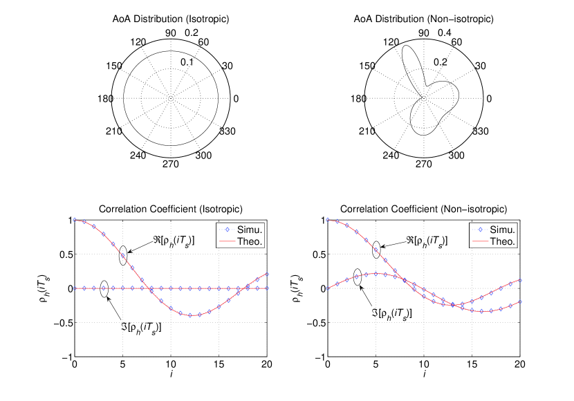
Figure 1: The AoA distributions for two scattering environments and the corresponding channel correlation coefficients.

The distributions of angle-of-arrival (AoA) for both scenarios and the corresponding channel correlation coefficients $\rho_{h}(iT_{\!s})$, $i\geq 0$, are plotted in Fig. 1, where “Simu.” means simulation, and “Theo.” refers to (57), with $f_{m}=10$ and $\tau=iT_{\!s}=\frac{i}{20f_{m}}$, $i=0,1,2,\cdots$.

In the following subsections, simulations are performed to verify the ACF, correlation coefficient, LCR and AOD of IMI in both types of environment at both low- and high-SNR regimes. For evaluating the approximation accuracy of ACF and the correlation coefficient, we set $\eta=-10$ dB for low SNR, and $\eta=30$ dB for high SNR. To verify the LCR and AOD expressions, $\eta=0,5,10$ dB are the SNRs considered.

VI-A Isotropic Scattering

This is the Clarke’s model, with uniform AoA. Simulations are performed for both SISO and the $2\times 2$ OSTBC-MIMO systems, with the results shown in Figs. 2 and 3, respectively.

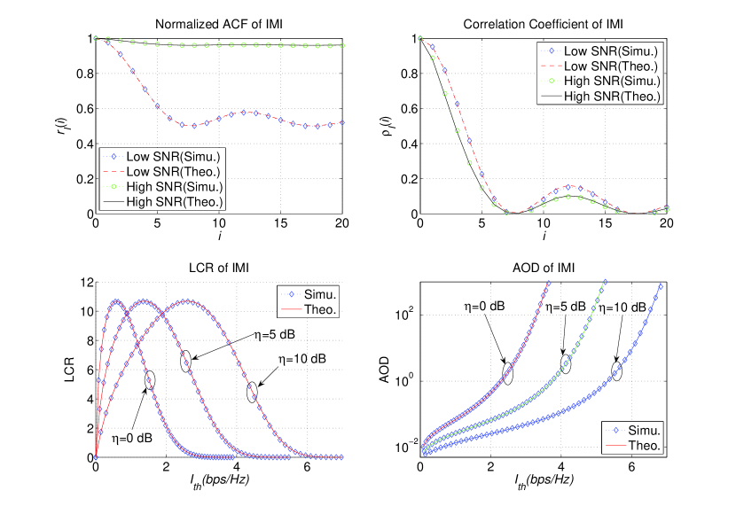
Figure 2: The ACF, correlation coefficient, LCR, and AOD of IMI in a SISO system with isotropic scattering.

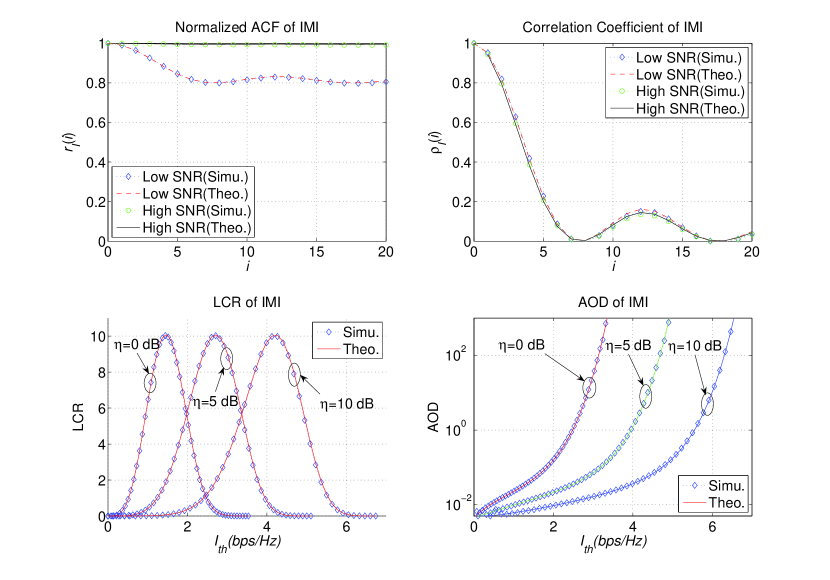
Figure 3: The ACF, correlation coefficient, LCR, and AOD of IMI in a $2\times 2$ OSTBC-MIMO system with isotropic scattering.

VI-B Non-isotropic Scattering

This is a general case, with an arbitrary AoA distribution. Simulations are also carried out for both SISO and the $2\times 2$ OSTBC-MIMO systems, with the results presented in Figs. 4 and 5, respectively.

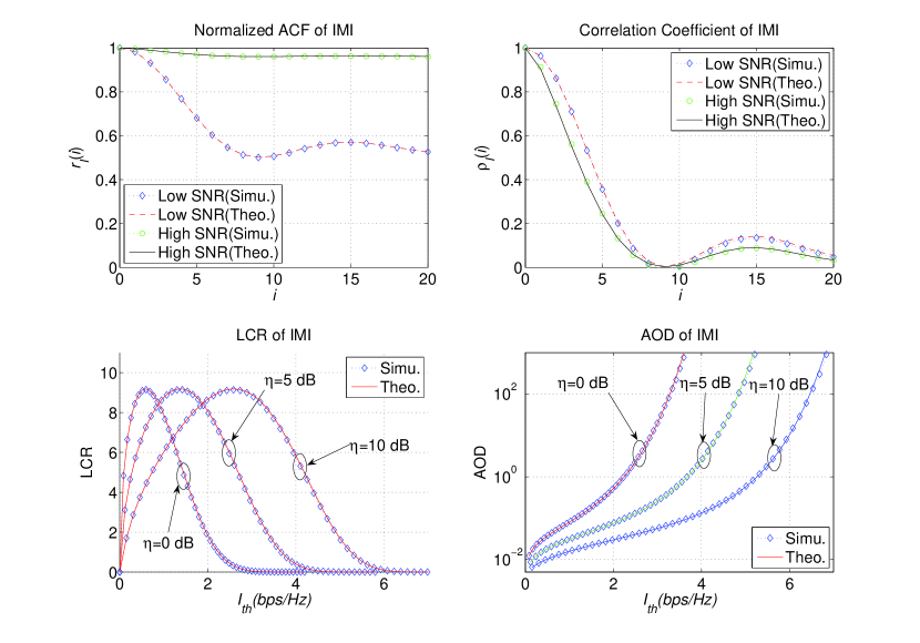
Figure 4: The ACF, correlation coefficient, LCR, and AOD of IMI in a SISO system with non-isotropic scattering.

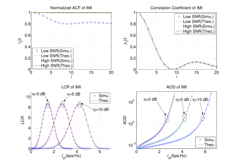
Figure 5: The ACF, correlation coefficient, LCR, and AOD of IMI in a $2\times 2$ OSTBC-MIMO system with non-isotropic scattering.

In Figs. 2-5, The upper left and right figures show the normalized approximate ACF and the approximate correlation coefficient of the IMI $\mathcal{I}_{l}$, respectively, in both low- and high-SNR regimes; the lower left is the LCR of $\mathcal{I}_{l}$, and finally, the lower right shows the AOD of $\mathcal{I}_{l}$. Moreover, in Figs. 2 and 4, for ACF, theoretical values in the low- and high-SNR regimes are calculated from (21) and (25), respectively. For the correlation coefficient, theoretical values come from (22) and (27), for low- and high-SNR regimes, respectively. The theoretical SISO LCR and AOD are given by (34) and (36), respectively. In Figs. 3 and 5, for ACF, theoretical values in the low- and high-SNR regimes are computed via (43) and (49), respectively. For the correlation coefficient, theoretical values come from (44) and (50) for low- and high-SNR regimes, respectively. The theoretical MIMO LCR and AOD are given by (53) and (48), respectively.

From Figs. 2-5, the following observations can be made.

• By comparing Figs. 2 and 4 for the SISO system, one can see larger peak values for LCR in the isotropic scattering case, which means more fluctuations of IMI. On the other hand, the AOD of IMI does not appear to be very sensitive to the differences among the propagation examples considered. The same conclusions apply to the $2\times 2$ OSTBC-MIMO system, depicted in Figs. 3 and 5.

• Based on the results shown in Figs. 2-5, for LCR and AOD we can conclude that the theoretical expressions perfectly match the simulations, in both propagation scenarios and for both SISO and $2\times 2$ OSTBC-MIMO systems. Moreover, the low- and high-SNR approximations for ACF and correlation coefficient are accurate in both types of systems and environments.

• Since in Figs. 3 and 5, the low-SNR approximation for $\rho_{\mathcal{I}}(i)$ is very close to the high-SNR approximation, one can conclude that $\rho_{\mathcal{I}}(i)\approx\varrho_{i}^{2}$ for any SNR in the OSTBC-MIMO systems with not-so-small number of antennas. This statement is further supported by the results shown in Table I, where for different values of $M\!N$, the Taylor series of $\rho_{\mathcal{I}}(i)$ in (46) is given, as well as maximum values $\max_{0\leq\varrho_{i}\leq 1}|(\ref{eq:Coeff_LowSNR_OSTBC})-(\ref{eq:Coeff_HighSNR_OSTBC})|$. From Table I, one can see that the larger the total number of antennas, the smaller the difference between (44) and (46). Moreover, even for $M\!N=2$, i.e., a MIMO system with two Tx and one Rx antennas, or one Tx and two Rx antennas, the difference is at most $0.075$, when using the approximation $\rho_{\mathcal{I}}(i)\approx\varrho_{i}^{2}$.

• According to Figs. 2 and 4, there is small gap between the SISO low- and high-SNR approximations of $\rho_{\mathcal{I}}(i)$, which is $0.16$ at most, shown in Table I. For the non-extreme SNR such as $10$ dB, the non-approximate $\rho_{\mathcal{I}}(i)$ in (14) can be used to calculate the correlation coefficient. However, by evaluating (14) and Monte Carlo simulations, we obtain the following simple approximation

  $$\rho_{\mathcal{I}}(i)\approx\begin{cases}\rho_{i}^{2},&\eta\leq 6.5\,\mathrm{dB},\\ \frac{\rho_{i}^{2}}{2}+\frac{3\operatorname{Li}_{2}\!\left(\varrho_{i}^{2}\right)}{\pi^{2}},&6.5\,\mathrm{dB}<\eta\leq 16\,\mathrm{dB},\\ \frac{6\operatorname{Li}_{2}\!\left(\varrho_{i}^{2}\right)}{\pi^{2}},&\eta>16\,\mathrm{dB},\end{cases}$$ (54)

  and the approximation error is $0.055$ at most.

VII Conclusion

In this paper, closed-form expressions for the level crossing rate and average outage duration of the instantaneous mutual information (IMI) in time-varying Rayleigh flat fading channels are derived, as well as the autocorrelation function and correlation coefficient of IMI, in SISO, MISO, SIMO and OSTBC-MIMO systems. The analytical expressions, supported by Monte Carlo simulations, provide useful qualitative and quantitative information regarding the fluctuations of IMI. For example, as the spread of the angle-of-arrival at the mobile receiver increases, the crossing rate of IMI increases, according to our results, which means faster fluctuation of IMI. Furthermore, IMI values become less correlated. Quantification of the average outage duration of IMI is another noteworthy outcome of this work. For example, with isotropic scattering, the IMI of a SISO system, with a $10$ dB SNR and $10$ Hz Doppler frequency, remains below $\mathcal{I}_{\text{th}}=6$ bps/Hz for almost $7$ seconds, on average, i.e., an average outage duration of $7$ seconds at the data rate $6$ bps/Hz.

Table I: Taylor Expansion of (46) and the Maximum Difference between (44) and (46) for Different $M\!N$’s

$M\!N$	$\text{Taylor Series of}\ (\ref{eq:Coeff_HighSNR_OSTBC})$	$\max_{0\leq\varrho_{i}\leq 1}|(\ref{eq:Coeff_LowSNR_OSTBC})-(\ref{eq:Coeff_HighSNR_OSTBC})|$
1	$0.608\varrho_{i}^{2}+0.152\varrho_{i}^{4}+\mathcal{O}(\varrho_{i}^{6})$	$0.16$
2	$0.775\varrho_{i}^{2}+0.129\varrho_{i}^{4}+\mathcal{O}(\varrho_{i}^{6})$	$0.075$
3	$0.844\varrho_{i}^{2}+0.106\varrho_{i}^{4}+\mathcal{O}(\varrho_{i}^{6})$	$0.048$
4	$0.881\varrho_{i}^{2}+0.088\varrho_{i}^{4}+\mathcal{O}(\varrho_{i}^{6})$	$0.035$
5	$0.904\varrho_{i}^{2}+0.075\varrho_{i}^{4}+\mathcal{O}(\varrho_{i}^{6})$	$0.027$
$\vdots$	$\vdots$	$\vdots$
16	$0.969\varrho_{i}^{2}+0.029\varrho_{i}^{4}+\mathcal{O}(\varrho_{i}^{6})$	$0.008$
$\vdots$	$\vdots$	$\vdots$
64	$0.992\varrho_{i}^{2}+0.008\varrho_{i}^{4}+\mathcal{O}(\varrho_{i}^{6})$	$0.002$

In this paper, we have not considered the spatially uncorrelated general MIMO system with $M$ transmitters and $N$ receivers, where all the subchannels are independent and identically distributed, with the same temporal correlation function. The mutual information in this case is given by[14] $\mathcal{I}_{l}=\log_{2}\det\!\left[\mathbf{I}_{N}+\frac{\eta}{M}\mathbf{H}(lT_{\!s})\mathbf{H}^{\dagger}(lT_{\!s})\right]$, where $\mathbf{H}(lT_{\!s})$ is the channel matrix at time $t=lT_{\!s}$. However, for low SNRs, it is straightforward to show that the MIMO IMI $\mathcal{I}_{l}$ is quite similar to the OSTBC-MIMO IMI, which means that the approximate normalized autocorrelation and correlation coefficient in (43) and (44) hold for more general MIMO systems as well. It is our ongoing work to derive closed-form expressions for the IMI autocorrelation function, correlation coefficient, LCR, and AOD of MIMO systems with any SNR, and also some high-SNR approximations.

Appendix A Channel and Angle-of-Arrival Models

In a flat Rayleigh fading channel, the lowpass complex envelope of the channel response $h(t)$ is a zero-mean complex Gaussian random process, which can be represented as

$$h(t)=h_{I}(t)+\jmath h_{Q}(t)=\alpha(t)\exp[-\jmath\Phi(t)],$$ (55)

where the zero-mean real Gaussian random processes $h_{I}(t)$ and $h_{Q}(t)$ are the real and imaginary parts of $h(t)$, respectively. $\alpha(t)$ is the envelope of $h(t)$ and $\Phi(t)$ is the phase of $h(t)$. At any time $t$, $\alpha(t)$ has a Rayleigh distribution and $\Phi(t)$ is distributed uniformly over $[0,2\pi)$. Without loss of generality, we assume the Rayleigh channel has unit power, i.e., $\mathbb{E}[\alpha^{2}(t)]=1$.

To model the distribution of the angle-of-arrival (AoA) of waves impinging either the base station (BS) or mobile station (MS), we use multiple von Mises distributions.

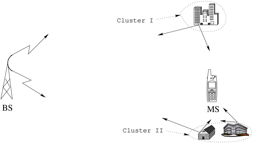
Figure 6: The scattering environment around the MS with two clusters of scatterers.

The von Mises PDF has proven to be a flexible AoA model for both BS[19] and MS[4]. For example, in the macrocellular environment shown in Fig. 6, two von Mises distributions are needed to model the two clusters of scatterers around the MS. In general, we write the PDF of AoA in the azimuth plane as the superposition of $K$ von Mises PDFs

$$p(\theta)=\sum_{n=1}^{K}P_{n}\frac{\exp[\kappa_{n}\cos(\theta-\theta_{n})]}{2\pi I_{0}(\kappa_{n})},\quad\theta\in[0,2\pi),$$ (56)

where $\theta_{n}$ is the mean AoA from the $n^{\text{th}}$ cluster, $\kappa_{n}$ controls the width of the $n^{\text{th}}$ cluster, and $P_{n}$ represents the contribution of the $n^{\text{th}}$ cluster, such that $\sum_{n=1}^{K}P_{n}=1,0<P_{n}\leq 1$. If $\kappa_{n}=0,\forall n$, (56) simplifies to $p(\theta)=\frac{1}{2\pi},\theta\in[0,2\pi)$, which is the Clarke’s two-dimensional isotropic scattering model. The AoA PDF given in (56) is general enough to model AoA distributions observed in practice. Furthermore, it provides closed-form and mathematically-tractable expressions for the channel correlation functions [19, 4].

The channel correlation coefficient $\rho_{h}(\tau)$ and the power spectrum of Rayleigh fading for the AoA model in (56) are given by

$$\rho_{h}(\tau) =\!E[h(t)h^{*}(t-\tau)],$$ (57)

$$=\!\sum_{n=1}^{K}\!P_{n}\!\frac{I_{0}\!\left(\!\sqrt{\kappa_{n}^{2}-4\pi^{2}f_{m}^{2}\tau^{2}+\jmath 4\pi\kappa_{n}f_{m}\tau\cos\theta_{n}}\right)}{I_{0}(\kappa_{n})},$$

and

$$S_{h}(f)=\sum_{n=1}^{K}P_{n}\frac{\exp(\kappa_{n}f\cos\theta_{n}/f_{m})}{\pi\sqrt{f_{m}^{2}-f^{2}}I_{0}(\kappa_{n})}\\ \times\cosh\!\left[\kappa_{n}\sqrt{1-(f/f_{m})^{2}}\sin\theta_{n}\right]\!\!,|f|\leq f_{m},$$ (58)

respectively, in which $f_{m}$ is the maximum Doppler frequency, and $\cosh(z)=\frac{1}{2}(e^{z}+e^{-z})$ is the hyperbolic cosine function. Equations (57) and (58) are derived by extending the results of [4], according to (56). If $\kappa_{n}=0,\forall n$, (57) and (58) simplify $\rho_{h}(\tau)=I_{0}(\jmath 2\pi f_{m}\tau)=J_{0}(2\pi f_{m}\tau)$ and $S_{h}(f)=\frac{1}{2\pi\sqrt{f_{m}^{2}-f^{2}}},|f|\leq f_{m}$, respectively, which correspond to the Clarke’s model.

Using (58) and the spectral method discussed in [18], the discrete-time version of $h(t)$, i.e., $h(lT_{\!s})$, is generated and used in Sec. VI to verify the accuracy of the new closed-form expressions derived in this paper.

Appendix B Derivation of (7), (8) and (14)

With (5) and (6) together, (4) can be written as

$$\frac{r_{\mathcal{I}}(i)}{(\log_{2}e)^{2}} =\int_{0}^{\infty}\!\!\!\!\int_{0}^{\infty}\bigg{[}\!\ln(1+\eta x_{1})\ln(1+\eta x_{2})$$

$$\ \times\lambda_{i}e^{-\lambda_{i}(x_{1}+x_{2})}\sum_{k=0}^{\infty}\frac{(\lambda_{i}\varrho_{i})^{2k}x_{1}^{k}x_{2}^{k}}{(k!)^{2}}\bigg{]}\mathrm{d}x_{1}\mathrm{d}x_{2},$$

$$=\lambda_{i}\sum_{k=0}^{\infty}\bigg{[}\frac{(\lambda_{i}\varrho_{i})^{2k}}{(k!)^{2}}\!\!\int_{0}^{\infty}\!\!\!x_{1}^{k}e^{-\lambda_{i}x_{1}}\ln(1+\eta x_{1})\mathrm{d}x_{1}$$

$$\ \times\int_{0}^{\infty}\!\!\!x_{2}^{k}e^{-\lambda_{i}x_{2}}\ln(1+\eta x_{2})\mathrm{d}x_{2}\bigg{]},$$

$$=\lambda_{i}\!\sum_{k=0}^{\infty}\!\!\frac{(\lambda_{i}\varrho_{i})^{2k}}{(k!)^{2}}\!\!\left[\!\int_{0}^{\infty}\!\!\!x^{k}e^{-\lambda_{i}x}\ln(1\!+\!\eta x)\mathrm{d}x\!\right]^{2}\!\!\!\!.$$ (59)

The exponential and logarithm functions can be represented by Meijer’s $G$ function as follows[20, (11)]

$$e^{-\lambda_{i}x}=G^{1,0}_{0,1}\!\left(\!\lambda_{i}x\left|\!\!\begin{array}[]{c}\cdot\\ 0\end{array}\right.\!\!\right),$$ (60)

and

$$\ln(1+\eta x)=G^{1,2}_{2,2}\!\left(\!\eta x\left|\!\!\begin{array}[]{c}1,1\\ 1,0\end{array}\right.\!\!\right).$$ (61)

Using the integral given in [20, (21)], the integral $\Xi(k,\eta,\lambda_{i})=\int_{0}^{\infty}x^{k}e^{-\lambda_{i}x}\ln(1+\eta x)\mathrm{d}x$ in (B) can be expressed in the following form

$$\begin{split}\Xi(k,\eta,\lambda_{i})&=\frac{1}{\eta^{k+1}}G_{2,3}^{3,1}\!\!\left(\!\frac{\lambda_{i}}{\eta}\left|\!\!\!\begin{array}[]{c}-(k\!+\!1),-k\\ -(k\!+\!1),-(k\!+\!1),0\end{array}\right.\!\!\!\!\right),\\ &=\frac{1}{\lambda_{i}^{k+1}}G_{2,3}^{3,1}\!\!\left(\!\frac{\lambda_{i}}{\eta}\left|\!\!\!\begin{array}[]{c}0,1\\ 0,0,k\!+\!1\end{array}\right.\!\!\!\!\right),\end{split}$$ (62)

where the last “=” comes from $z^{k}G_{p,q}^{m,n}\!\!\left(z\left|\!\begin{array}[]{c}(a_{p})\\ (b_{q})\end{array}\right.\!\!\!\right)=G_{p,q}^{m,n}\!\!\left(z\left|\!\begin{array}[]{c}k+(a_{p})\\ k+(b_{q})\end{array}\right.\!\!\!\right)$[21, pp. 521, 8.2.2.15], in which $(a_{p})=a_{1},a_{2},\cdots,a_{p}$ and $(b_{q})=b_{1},b_{2},\cdots,b_{q}$. By substituting (62) into (B), we obtain (7).

To obtain (8) and (14), we need to calculate $\frac{\mathbb{E}\left[\mathcal{I}_{l}\right]}{\log_{2}e}=\mathbb{E}\left[\ln(1+\eta x_{1})\right]$ and $\mathbb{E}\left[\mathcal{I}_{l}^{2}\right]=(\log_{2}\!e)^{2}\mathbb{E}\left[\ln^{2}(1+\eta x_{1})\right]$. With $p(x_{1})=e^{-x_{1}}$, $x_{1}\geq 0$, the characteristic function of $\ln(1+\eta x_{1})$ is given by

$$\begin{split}\xi_{\mathcal{I}}(t)&=\mathbb{E}\left[e^{\jmath t\ln(1+\eta x_{1})}\right]=\int_{0}^{\infty}e^{-x_{1}}(1+\eta x_{1})^{\jmath t}\,\mathrm{d}x_{1},\\ &\operatornamewithlimits{=}^{z=\frac{1}{\eta}+x_{1}}\eta^{\jmath t}e^{\frac{1}{\eta}}\int_{\frac{1}{\eta}}^{\infty}z^{\jmath t}e^{-z}\mathrm{d}z=\eta^{\jmath t}e^{\frac{1}{\eta}}\Gamma\left(\jmath t+1,\frac{1}{\eta}\right).\end{split}$$ (63)

The first and second moments of $\ln(1+\eta x_{1})$ are obtained as

$$\mathbb{E}\left[\ln(1+\eta x_{1})\right]=\frac{1}{\jmath}\left.\frac{\partial\xi_{\mathcal{I}}(t)}{\partial t}\right|_{t=0}=e^{\frac{1}{\eta}}\Gamma\left(0,\frac{1}{\eta}\right),$$ (64)

and

$$\begin{split}\mathbb{E}\left[\ln^{2}\!(1\!+\!\eta x_{1})\right]&=\frac{1}{\jmath^{2}}\!\!\left.\frac{\partial^{2}\xi_{\mathcal{I}}(t)}{\partial t^{2}}\right|_{t=0},\\ &=2e^{\frac{1}{\eta}}G_{2,3}^{3,0}\!\!\left(\!\frac{1}{\eta}\!\left|\!\begin{array}[]{c}1,1\\ 0,0,0\end{array}\right.\!\!\!\right),\end{split}$$ (65)

respectively. With (64) and (65), we easily obtain (8) and (14).

Appendix C Derivation of (25) and (26)

By plugging (24) into (23) we obtain

$$\begin{split}\frac{r_{\mathcal{I}}(i)}{(\log_{2}e)^{2}}&\approx\frac{1}{\lambda_{i}}\!\sum_{k=0}^{\infty}\varrho_{i}^{2k}\left(\ln\frac{\eta}{\lambda_{i}\gamma}+{H}_{\!k}\right)^{2},\\ &=\frac{1}{\lambda_{i}}\left[S_{2}(\varrho_{i}^{2})+2S_{1}(\varrho_{i}^{2})\ln\frac{\eta}{\lambda_{i}\gamma}+S_{0}(\varrho_{i}^{2})\ln^{2}\frac{\eta}{\lambda_{i}\gamma}\right],\end{split}$$ (66)

where[22]

$$S_{0}(\varrho_{i}^{2}) =\sum_{k=0}^{\infty}\varrho_{i}^{2k},$$

$$=\lambda_{i},$$ (67a)

$$S_{1}(\varrho_{i}^{2}) =\sum_{k=0}^{\infty}{H}_{\!k}\varrho_{i}^{2k},$$

$$=\lambda_{i}\ln\lambda_{i},$$ (67b)

$$S_{2}(\varrho_{i}^{2}) =\sum_{k=0}^{\infty}{H}_{\!k}^{2}\varrho_{i}^{2k},$$

$$=\lambda_{i}\left[\operatorname{Li}_{2}\!\left(\varrho_{i}^{2}\right)+\ln^{2}\lambda_{i}\right].$$ (67c)

Substitution of (67) into (66) yields

$$\frac{r_{\mathcal{I}}(i)}{(\log_{2}e)^{2}}=\operatorname{Li}_{2}\!\left(\varrho_{i}^{2}\right)+\ln^{2}\frac{\eta}{\gamma}.$$ (68)

After normalization, i.e., $\tilde{r}_{\mathcal{I}}(i)=\frac{r_{\mathcal{I}}(i)}{r_{\mathcal{I}}(0)}$, where $r_{\mathcal{I}}(0)\approx(\log_{2}e)^{2}\left(\frac{\pi^{2}}{6}+\ln^{2}\frac{\eta}{\gamma}\right)$, (68) reduces to (25).

The correlation coefficient is calculated as follows

$$\begin{split}\rho_{\mathcal{I}}(i)&\approx\frac{r_{\mathcal{I}}(i)-\left\{\left(\log_{2}e\right)\mathbb{E}[\ln(\eta x_{1})]\right\}^{2}}{r_{\mathcal{I}}(0)-\left\{\left(\log_{2}e\right)\mathbb{E}[\ln(\eta x_{1})]\right\}^{2}},\\ &\approx\frac{\operatorname{Li}_{2}\!\left(\varrho_{i}^{2}\right)+\ln^{2}\frac{\eta}{\gamma}-\ln^{2}\frac{\eta}{\gamma}}{\frac{\pi^{2}}{6}+\ln^{2}\frac{\eta}{\gamma}-\ln^{2}\frac{\eta}{\gamma}},\\ &=\frac{6\operatorname{Li}_{2}\!\left(\varrho_{i}^{2}\right)}{\pi^{2}},\end{split}$$ (69)

where the second line is from the fact that $\mathbb{E}\left[\ln(\eta x_{1})\right]=\ln\eta+\int_{0}^{\infty}e^{-x_{1}}\ln x_{1}\,\mathrm{d}x_{1}=\ln\frac{\eta}{\gamma}$ using $\int_{0}^{\infty}e^{-x_{1}}\ln x_{1}\,\mathrm{d}x_{1}=-\ln\gamma$[11, pp. 602, 4.331.1].

Appendix D Derivation of Some Results in Sec. V

D-A Derivation of (38) and (39)

Substitution of (37c) and (41) into (3) results in

$$\frac{r_{\mathcal{I}}(i)}{(\log_{2}e)^{2}} =\int_{0}^{\infty}\int_{0}^{\infty}\Bigg{[}\ln\left(1+\frac{\eta}{M}y_{1}\right)\ln\left(1+\frac{\eta}{M}y_{2}\right)$$

$$\hskip 10.00002pt\times\frac{\lambda_{i}^{M\!N}(y_{1}y_{2})^{M\!N-1}e^{-\lambda_{i}(y_{1}+y_{2})}}{(M\!N-1)!}$$

$$\hskip 10.00002pt\times\sum_{k=0}^{\infty}\frac{(\lambda_{i}\varrho_{i})^{2k}(y_{1}y_{2})^{k}}{k!(M\!N+k-1)!}\Bigg{]}\mathrm{d}y_{1}\mathrm{d}y_{2},$$

$$=\frac{\lambda_{i}^{M\!N}}{(M\!N-1)!}\sum_{k=0}^{\infty}\Bigg{[}\frac{(\lambda_{i}\varrho_{i})^{2k}}{k!(M\!N+k-1)!}$$

$$\hskip 10.00002pt\times\int_{0}^{\infty}y_{1}^{k+M\!N-1}e^{-\lambda_{i}y_{1}}\ln\left(1+\frac{\eta}{M}y_{1}\right)\mathrm{d}y_{1}$$

$$\hskip 10.00002pt\times\int_{0}^{\infty}y_{2}^{k+M\!N-1}e^{-\lambda_{i}y_{2}}\ln\left(1+\frac{\eta}{M}y_{2}\right)\mathrm{d}y_{2}\Bigg{]},$$

$$=\frac{\lambda_{i}^{M\!N}}{(M\!N-1)!}\sum_{k=0}^{\infty}\Bigg{\{}\frac{(\lambda_{i}\varrho_{i})^{2k}}{k!(M\!N+k-1)!}$$

$$\times\left[\int_{0}^{\infty}y_{1}^{k+M\!N-1}e^{-\lambda_{i}y_{1}}\ln\left(1+\frac{\eta}{M}y_{1}\right)\mathrm{d}y_{1}\right]^{2}\Bigg{\}},$$

$$=\frac{\lambda_{i}^{-M\!N}}{(M\!N-1)!}\sum_{k=0}^{\infty}\frac{\varrho_{i}^{2k}\left[G_{2,3}^{3,1}\!\!\left(\!\frac{M\lambda_{i}}{\eta}\!\left|\!\!\begin{array}[]{c}0,1\\ 0,0,k\!+\!M\!N\end{array}\right.\!\!\!\!\right)\right]^{2}}{k!(M\!N+k-1)!}.$$ (72)

For calculating the normalized ACF and the correlation coefficient, we need the first and second moments of $\mathcal{I}_{l}$, i.e., $\mathbb{E}\left[\ln\left(1+\frac{\eta}{M}y_{1}\right)\right]$ and $\mathbb{E}\left[\ln^{2}\left(1+\frac{\eta}{M}y_{1}\right)\right]$. Using the integral results given in (62), we have the first moment as

$$\mathbb{E}\left[\ln\left(1+\frac{\eta}{M}y_{1}\right)\right] =\int_{0}^{\infty}\frac{y_{1}^{M\!N-1}e^{-y_{1}}}{(M\!N-1)!}\ln\left(1+\frac{\eta}{M}y_{1}\right)\mathrm{d}y_{1},$$

$$=\frac{G_{2,3}^{3,1}\!\left(\!\frac{M}{\eta}\!\left|\begin{array}[]{c}0,1\\ 0,0,M\!N\end{array}\right.\!\!\right)}{(M\!N\!-\!1)!}.$$ (75)

The second moment is given in (69), where the third “=” is based on the integral identity 4.358.1 in [11, pp. 607].

$$\begin{split}\mathbb{E}\left[\ln^{2}\left(1+\frac{\eta}{M}y_{1}\right)\right]&=\int_{0}^{\infty}\frac{y_{1}^{M\!N-1}e^{-y_{1}}}{(M\!N-1)!}\ln^{2}\left(1+\frac{\eta}{M}y_{1}\right)\mathrm{d}y_{1},\\ &\operatornamewithlimits{=}^{z=1+\frac{\eta}{M}y_{1}}\frac{e^{\frac{M}{\eta}}\sum_{j=0}^{M\!N-1}{M\!N-1\choose j}(-1)^{M\!N-1-j}\int_{1}^{\infty}z^{j}e^{-\frac{M}{\eta}z}\ln^{2}z\mathrm{d}z}{(M\!N\!-\!1)!\left(\frac{\eta}{M}\right)^{M\!N}},\\ &=\frac{e^{\frac{M}{\eta}}\sum_{j=0}^{M\!N-1}{M\!N-1\choose j}(-1)^{M\!N-1-j}\frac{\partial^{2}}{\partial\nu^{2}}\!\!\left.\left[\!\left(\frac{M}{\eta}\right)^{-\nu}\Gamma\!\left(\nu,\frac{M}{\eta}\right)\!\right]\!\right|_{\nu=j+1}}{(M\!N\!-\!1)!\left(\frac{\eta}{M}\right)^{M\!N}},\\ &=\frac{2e^{\frac{M}{\eta}}{\displaystyle\sum_{j=0}^{M\!N-1}}{M\!N-1\choose j}(-1)^{M\!N-1-j}G_{3,4}^{4,0}\!\left(\!\frac{M}{\eta}\!\left|\begin{array}[]{c}-\!j,-\!j,-\!j\\ 0,-\!j\!-\!1,-\!j\!-\!1,-\!j\!-\!1\end{array}\right.\!\!\!\!\right)}{(M\!N\!-\!1)!\left(\frac{\eta}{M}\right)^{M\!N}}.\end{split}$$ (69)

D-B Derivation of (43) and (44)

For calculating the low-SNR approximation for the normalized ACF and the correlation coefficient, the following lemma is necessary.

Lemma 1

If $|t|<1$ and $p$ is a non-negative integer, then the following identity holds.

$$\sum_{k=0}^{\infty}\frac{(k+p)!(k+p)}{k!}t^{k}=\frac{(p+t)p!}{(1-t)^{p+2}}.$$ (76)

Proof:

For $p=0$, obviously it holds[11, pp. 8, 0.231.2].

For $p\geq 1$ we have

$$\begin{split}\sum_{k=0}^{\infty}\frac{(k+p)!(k+p)}{k!}t^{k}&=\frac{\partial^{p-1}}{\partial t^{p-1}}\left[t^{p-1}\sum_{k=0}^{\infty}(k+p)^{2}t^{k}\right],\\ &=\frac{\partial^{p-1}}{\partial t^{p-1}}\left[\frac{\partial}{\partial t}\sum_{k=0}^{\infty}(k+p)t^{k+p}\right]=\frac{\partial^{p}}{\partial t^{p}}\left[t\frac{\partial}{\partial t}\sum_{k=0}^{\infty}t^{k+p}\right],\\ &=\frac{\partial^{p}}{\partial t^{p}}\left[t\frac{\partial}{\partial t}\frac{t^{p}}{1-t}\right]=\frac{\partial^{p}}{\partial t^{p}}\left[\frac{t^{p}(p-pt+t)}{(1-t)^{2}}\right]=\frac{(p+t)p!}{(1-t)^{p+2}},\end{split}$$

where the fourth “=” is from $\sum_{k=0}^{\infty}t^{k+p}=\frac{t^{p}}{1-t}$, when $|t|<1$ and $p$ is an positive integer. ∎

Using the low-SNR approximation, similar to (15) in the SISO case, with $x$, $k$, and $\eta$ replaced by $y_{1}$, $k+M\!N-1$, and $\eta/M$, respectively, (D-A) reduces to

$$\frac{r_{\mathcal{I}}(i)}{(\log_{2}e)^{2}} \approx\frac{\eta^{2}\lambda_{i}^{M\!N}}{M^{2}(M\!N-1)!}\sum_{k=0}^{\infty}\Bigg{\{}\frac{(\lambda_{i}\varrho_{i})^{2k}}{k!(M\!N+k-1)!}$$

$$\hskip 10.00002pt\times\left[\int_{0}^{\infty}y_{1}^{k+M\!N}e^{-\lambda_{i}y_{1}}\mathrm{d}y_{1}\right]^{2}\Bigg{\}},$$

$$=\frac{\eta^{2}\lambda_{i}^{M\!N}}{M^{2}(M\!N-1)!}\sum_{k=0}^{\infty}\frac{(\lambda_{i}\varrho_{i})^{2k}}{k!(M\!N+k-1)!}\left[\frac{(k+M\!N)!}{\lambda_{i}^{k+M\!N+1}}\right]^{2},$$

$$=\frac{\eta^{2}}{M^{2}(M\!N-1)!\lambda_{i}^{M\!N+2}}\sum_{k=0}^{\infty}\frac{(k+M\!N)!(k+M\!N)}{k!}(\varrho_{i}^{2})^{k},$$

$$=\frac{\eta^{2}N(M\!N+\varrho_{i}^{2})}{M},$$ (78)

where the last “=” is from Lemma 1. Therefore we have the approximate normalized ACF as given in (43). For the approximate correlation coefficient we obtain

$$\begin{split}\rho_{\mathcal{I}}(i)&\approx\frac{r_{\mathcal{I}}(i)-\left\{\left(\log_{2}e\right)\mathbb{E}\left[\frac{\eta}{M}y\right]\right\}^{2}}{r_{\mathcal{I}}(0)-\left\{\left(\log_{2}e\right)\mathbb{E}\left[\frac{\eta}{M}y\right]\right\}^{2}},\\ &=\frac{\frac{\eta^{2}N(M\!N+\varrho_{i}^{2})}{M}-\eta^{2}N^{2}}{\frac{\eta^{2}N(M\!N+1)}{M}-\eta^{2}N^{2}}=\varrho_{i}^{2},\end{split}$$ (79)

where $\mathbb{E}[y_{1}]=M\!N$[17, pp. 14, (2.35)] is used in the second line of (79).

D-C Derivation of (45) and (46)

For the high-SNR regime, the approximation of $\frac{r_{\mathcal{I}}(i)}{(\log_{2}e)^{2}}$ is detailed in (D-C), where a high-SNR approximation similar to (15) in the SISO case is used, and $R_{j}(\varrho_{i}^{2})$, $j=0,1,2$, are given in (81), (83), and (84), respectively.

$$\frac{r_{\mathcal{I}}(i)}{(\log_{2}e)^{2}} =\frac{\lambda_{i}^{M\!N}}{(M\!N-1)!}\sum_{k=0}^{\infty}\frac{(\lambda_{i}\varrho_{i})^{2k}}{k!(M\!N+k-1)!}\left[\int_{0}^{\infty}y_{1}^{k+M\!N-1}e^{-\lambda_{i}y_{1}}\ln\left(1+\frac{\eta}{M}y_{1}\right)\mathrm{d}y_{1}\right]^{2},$$

$$\approx\frac{\lambda_{i}^{M\!N}}{(M\!N-1)!}\sum_{k=0}^{\infty}\frac{(\lambda_{i}\varrho_{i})^{2k}}{k!(M\!N+k-1)!}\left[\int_{0}^{\infty}y_{1}^{k+M\!N-1}e^{-\lambda_{i}y_{1}}\ln\left(\frac{\eta}{M}y_{1}\right)\mathrm{d}y_{1}\right]^{2},$$

$$=\frac{\lambda_{i}^{M\!N}}{(M\!N-1)!}\sum_{k=0}^{\infty}\frac{(\lambda_{i}\varrho_{i})^{2k}}{k!(M\!N+k-1)!}\left[\frac{(k+M\!N-1)!}{\lambda_{i}^{k+M\!N}}\left(\ln\frac{\eta}{M\lambda_{i}\gamma}+{H}_{\!k+M\!N-1}\right)\right]^{2},$$

$$=\frac{1}{(M\!N-1)!\lambda_{i}^{M\!N}}\sum_{k=0}^{\infty}\frac{(k+M\!N-1)!(\varrho_{i}^{2})^{k}}{k!}\left(\ln\frac{\eta}{M\lambda_{i}\gamma}+{H}_{\!k+M\!N-1}\right)^{2},$$

$$=\frac{1}{(M\!N-1)!\lambda_{i}^{M\!N}}\left[R_{2}(\varrho_{i}^{2})+2R_{1}(\varrho_{i}^{2})\ln\frac{\eta}{M\lambda_{i}\gamma}+R_{0}(\varrho_{i}^{2})\ln^{2}\frac{\eta}{M\lambda_{i}\gamma}\right].$$ (77)

In what follows, we focus on how to calculate the three infinite summations $R_{j}(t),j=0,1,2,|t|<1$, introduced in (D-C). First, we consider $R_{0}(t)$

$$R_{0}(t) =\sum_{k=0}^{\infty}\!\frac{(k\!+\!M\!N\!-\!1)!t^{k}}{k!}=\sum_{k=0}^{\infty}\frac{\partial^{M\!N-1}}{\partial t^{M\!N-1}}t^{k+M\!N-1},$$

$$=\frac{\partial^{M\!N-1}}{\partial t^{M\!N-1}}\sum_{k=0}^{\infty}t^{k+M\!N-1}=\frac{\partial^{M\!N-1}}{\partial t^{M\!N-1}}\left(\sum_{k=0}^{\infty}t^{k}-\sum_{k=0}^{M\!N-2}t^{k}\right),$$

$$=\frac{\partial^{M\!N-1}}{\partial t^{M\!N-1}}\sum_{k=0}^{\infty}t^{k}\operatornamewithlimits{=}^{|t|<1}\frac{\partial^{M\!N-1}S_{0}(t)}{\partial t^{M\!N-1}}=\frac{(M\!N-1)!}{(1-t)^{M\!N}},$$ (80)

where we use $S_{0}(t)=\frac{1}{1-t}$ in (67a). Therefore we have

$$R_{0}(\varrho_{i}^{2})=\sum_{k=0}^{\infty}\frac{(k+M\!N-1)!}{k!}\varrho_{i}^{2k}=\frac{(M\!N-1)!}{(1-\varrho_{i}^{2})^{M\!N}}.$$ (81)

With the same reasoning we obtain

$$R_{j}(t)=\frac{\partial^{M\!N-1}S_{j}(t)}{\partial t^{M\!N-1}},j=1,2,$$ (82)

where $S_{j}(t),j=1,2$, are given by (67b) and (67c), respectively. Hence

$$R_{1}(\varrho_{i}^{2}) =\sum_{k=0}^{\infty}\frac{(k+M\!N-1)!}{k!}{H}_{\!k+M\!N-1}\varrho_{i}^{2k},$$

$$=\frac{\partial^{M\!N-1}}{\partial t^{M\!N-1}}\left.\left[-\frac{\ln(1-t)}{(1-t)}\right]\right|_{t=\varrho_{i}^{2}},$$

$$=\frac{(M\!N-1)!\left[{H}_{\!M\!N-1}-\ln(1-\varrho_{i}^{2})\right]}{(1-\varrho_{i}^{2})^{M\!N}},$$ (83)

$$R_{2}(\varrho_{i}^{2}) =\sum_{k=0}^{\infty}\frac{(k+M\!N-1)!}{k!}{H}_{\!k+M\!N-1}^{2}\varrho_{i}^{2k},$$

$$=\frac{\partial^{M\!N-1}}{\partial t^{M\!N-1}}\left.\left[\frac{\operatorname{Li}_{2}(t)+\ln^{2}(1-t)}{(1-t)}\right]\right|_{t=\varrho_{i}^{2}}.$$ (84)

The second moment of $\ln\left(\frac{\eta}{M}y\right)$ is given by

$$\frac{r_{\mathcal{I}}(0)}{(\log_{2}e)^{2}} \approx\int_{0}^{\infty}\frac{y_{1}^{M\!N-1}e^{-y_{1}}}{(M\!N-1)!}\ln^{2}\frac{\eta}{M}y_{1}\mathrm{d}y_{1},$$

$$\operatornamewithlimits{=}^{z=\frac{\eta}{M}y_{1}}\frac{\left(\frac{M}{\eta}\right)^{M\!N}}{(M\!N-1)!}\int_{0}^{\infty}z^{M\!N-1}e^{-\frac{M}{\eta}z}\ln^{2}z\mathrm{d}z,$$

$$=\left({H}_{\!M\!N-1}+\ln\frac{\eta}{M\gamma}\right)^{2}+\zeta(2,M\!N),$$ (86)

in which the last “=” is from 4.358.2 [11, pp. 607], where in [11] $\psi(q)={H}_{\!q-1}-\ln\gamma$, with $q$ as a positive integer[11, pp. 952, 8.365.4]. Therefore, we obtain (45) for the normalized ACF. With

$$\begin{split}\mathbb{E}\left[\ln\left(\frac{\eta}{M}y\right)\right]&=\int_{0}^{\infty}\frac{y_{1}^{M\!N-1}e^{-y_{1}}}{(M\!N-1)!}\ln\left(\frac{\eta}{M}y_{1}\right)\mathrm{d}y_{1},\\ &=\ln\frac{\eta}{M\gamma}+{H}_{\!M\!N-1},\end{split}$$ (87)

where the last “=” is from (24), we have (46) for the correlation coefficient.

References

- [1] W. C. Jakes, Ed., Microwave Mobile Communications. New York: IEEE Press, 1994.
- [2] A. Abdi, K. Wills, H. A. Barger, M. S. Alouini, and M. Kaveh, “Comparison of the level crossing rate and average fade duration of Rayleigh, Rice, and Nakagami fading models with mobile channel data,” in Proc. IEEE Veh. Technol. Conf., Boston, MA, 2000, pp. 1850–1857.
- [3] N. Youssef, T. Munakata, and M. Takeda, “Fade statistics in Nakagami fading environments,” in Proc. IEEE Int. Symp. Spread Spec. Tech. App., Mainz, Germany, 1996, pp. 1244–1247.
- [4] A. Abdi, J. A. Barger, and M. Kaveh, “A parametric model for the distribution of the angle of arrival and the associated correlation function and power spectrum at the mobile station,” IEEE Trans. Veh. Technol., vol. 51, pp. 425–434, May 2002.
- [5] A. Abdi, W. C. Lau, M. S. Alouini, and M. Kaveh, “A new simple model for land mobile satellite channels: First- and second-order statistics,” IEEE Trans. Wireless Commun., vol. 2, pp. 519–528, May 2003.
- [6] L. H. Ozarow, S. Shamai, and A. D. Wyner, “Information theoretic considerations for cellular mobile radio,” IEEE Trans. Veh. Technol., vol. 43, pp. 359–378, May 1994.
- [7] D. Tse and P. Viswanath, Fundamentals of Wireless Communication. Cambridge, UK: Cambridge University Press, 2005.
- [8] A. Giorgetti, M. Chiani, M. Shafi, and P. J. Smith, “Level crossing rates and MIMO capacity fades: impacts of spatial/temporal channel correlation,” in Proc. IEEE Int. Conf. Commun., Anchorage, AK, 2003, pp. 3046–3050.
- [9] N. Zhang and B. Vojcic, “Evaluating the temporal correlation of MIMO channel capacities,” in Proc. IEEE Global Telecommun. Conf., St. Louis, MO, 2005, pp. 2817–2821.
- [10] W. B. Davenport and W. L. Root, An Introduction to the Theory of Random Signals and Noise. New York: Wiley, 1987.
- [11] I. S. Gradshteyn, I. M. Ryzhik, and A. Jeffrey, Eds., Table of Integrals, Series, and Products, 5th ed. San Diego, CA: Academic, 1994.
- [12] R. L. Graham, D. E. Knuth, and O. Patashnik, Eds., Concrete Mathematics: A Foundation for Computer Science, 2nd ed. Boston, MA: Addison-Wesley, 1994.
- [13] B. Kedem, Time Series Analysis by Higher Order Crossings. New York: IEEE Press, 1994.
- [14] İ. E. Telatar, “Capaicty of multi-antenna Gaussian channels,” European Trans. Telecommun., vol. 10, pp. 585–595, 1999.
- [15] E. G. Larsson and P. Stoica, Space-Time Block Coding for Wireless Communications. Cambridge, UK: Cambridge University Press, 2003.
- [16] A. Paulraj, R. Nabar, and D. Gore, Introduction to Space-Time Wireless Communications. Cambridge, UK: Cambridge University Press, 2003.
- [17] M. K. Simon, Probability Distributions Involving Gaussian Random Variables: A Handbook for Engineers and Scientists. Boston, MA: Kluwer, 2002.
- [18] K. Acolatse and A. Abdi, “Efficient simulation of space-time correlated MIMO mobile fading channels,” in Proc. IEEE Veh. Technol. Conf., Orlando, FL, 2003, pp. 652–656.
- [19] A. Abdi and M. Kaveh, “A versatile spatio-temporal correlation function for mobile fading channels with non-isotropic scattering,” in Proc. IEEE Workshop Statistical Signal Array Processing, Pocono Manor, PA, 2000, pp. 58–62.
- [20] V. S. Adamchik and O. I. Marichev, “The algorithm for calculating integrals of hypergeometric type functions and its realization in REDUCE system,” in Proc. Int. Conf. Symbolic Algebraic Computation, Tokyo, Japan, 1990, pp. 212–224.
- [21] A. P. Prudnikov, Yu A. Brychkov, and O. I. Marichev, Integraly i ryady. V 3 t. Tom. 3. Specialьnye funkcii. Dopolnitelьnye glavy., 2nd ed. MOSKVA: FIMATLIT, 2003.
- [22] B. de Neumann, “An interesting result arising from the analysis of diversity receivers,” Bull. IMA, vol. 27, pp. 48–50, Mar. 1991.