Towards Low-Complexity Linear-Programming Decoding

Abstract

We consider linear-programming (LP) decoding of low-density parity-check (LDPC) codes. While it is clear that one can use any general-purpose LP solver to solve the LP that appears in the decoding problem, we argue in this paper that the LP at hand is equipped with a lot of structure that one should take advantage of. Towards this goal, we study the dual LP and show how coordinate-ascent methods lead to very simple update rules that are tightly connected to the min-sum algorithm. Moreover, replacing minima in the formula of the dual LP with soft-minima one obtains update rules that are tightly connected to the sum-product algorithm. This shows that LP solvers with complexity similar to the min-sum algorithm and the sum-product algorithm are feasible. Finally, we also discuss some sub-gradient-based methods.

I Introduction

Linear-programming (LP) decoding [1, 2] has recently emerged as an interesting option for decoding low-density parity-check (LDPC) codes. Indeed, the observations in  [3, 4, 5] suggest that the LP decoding performance is very close to the message-passing iterative (MPI) decoding performance. Of course, one can use any general-purpose LP solver to solve the LP that appears in LP decoding, however in this paper we will argue that one should take advantage of the special structure of the LP at hand in order to formulate efficient algorithms that provably find the optimum of the LP.

Feldman et al. [6] briefly mention the use of sub-gradient methods for solving the LP of an early version of the LP decoder (namely for turbo-like codes). Moreover, Yang et al. [7] present a variety of interesting approaches to solve the LP where they use some of the special features of the LP at hand. However, we belive that one can take much more advantage of the structure that is present: this paper shows some results in that direction.

So far, MPI decoding has been successfully used in applications where block error rates on the order of $10^{-5}$ are needed because for these block error rates the performance of MPI decoding can be guaranteed by simulation results. However, for applications like magnetic recording, where one desires to have block error rates on the order of $10^{-15}$ and less, it is very difficult to guarantee that MPI decoding achieves such low block error rates for a given signal-to-noise ratio. The problem is that simulations are too time-consuming and that the known analytical results are not strong enough. Our hope and main motivation for the present work is that efficient LP decoders, together with analytical results on LP decoding (see e.g. [8, 9, 10]), can show that efficient decoders exist for which low block error rates can be guaranteed for a certain signal-to-noise ratio.

This paper is structured as follows. We start off by introducing in Sec. II the primal LP that appears in LP decoding. In Sec. III we formulate the dual LP and in Secs. IV and V we consider a “softened” version of this dual LP. Then, in Secs. VI and VII we propose some efficient decoding algorithms and in Sec. VIII we show some simulation results. Finally, in Sec. IX we offer some conclusions and in the appendix we present the proofs and some additional material.

Before going to the main part of the paper, let us fix some notation. We let $\mathbb{R}$, $\mathbb{R}_{+}$, and $\mathbb{R}_{++}$ be the set of real numbers, the set of non-negative real numbers, and the set of positive real numbers, respectively. Moreover, we will use the canonical embedding of the set $\mathbb{F}_{2}=\{0,1\}$ into $\mathbb{R}$. The convex hull of a set $\mathcal{A}\subseteq\mathbb{R}^{n}$ is denoted by $\operatorname{conv}(\mathcal{A})$. If $\mathcal{A}$ is a subset of $\mathbb{F}_{2}^{n}$ then $\operatorname{conv}(\mathcal{A})$ denotes the convex hull of the set $\mathcal{A}$ after $\mathcal{A}$ has been canonically embedded in $\mathbb{R}^{n}$. The $i$-th component of a vector $\mathbf{x}$ will be called $[\mathbf{x}]_{i}$ and the element in the $j$-th row and $i$-th column of a matrix $\mathbf{A}$ will be called $[\mathbf{A}]_{j,i}$.

Moreover, we will use Iverson’s convention, i.e. for a statement $A$ we have $[A]=1$ if $A$ is true and $[A]=0$ otherwise. From this we also derive the notation $\big{\llbracket}A\big{\rrbracket}\triangleq-\log[A]$, i.e. $\big{\llbracket}A\big{\rrbracket}=0$ if $A$ is true and $\big{\llbracket}A\big{\rrbracket}=+\infty$ otherwise. Let $\mathcal{A}$ and $\mathcal{X}$ be some arbitrary sets fulfilling $\mathcal{A}\subseteq\mathcal{X}$. A function like $\mathcal{X}\to\mathbb{R}_{+}:\mathbf{x}\mapsto[\mathbf{x}\in\mathcal{A}]$ is called an indicator function for the set $\mathcal{A}$, whereas a function like $\mathcal{X}\to\mathbb{R}_{+}:\mathbf{x}\mapsto\big{\llbracket}\mathbf{x}\in\mathcal{A}\big{\rrbracket}$ is called a neglog indicator function for the set $\mathcal{A}$. Of course, this second function can also be considered as a cost or penalty function.

Throughout the paper, we will consider a binary linear code $\mathcal{C}$ that is defined by a parity-check matrix $\mathbf{H}$ of size $m$ by $n$. Based on $\mathbf{H}$, we define the sets $\mathcal{I}\triangleq\mathcal{I}(\mathbf{H})\triangleq\{1,\ldots,n\}$, $\mathcal{J}\triangleq\mathcal{J}(\mathbf{H})\triangleq\{1,\ldots,m\}$, $\mathcal{I}_{j}\triangleq\mathcal{I}_{j}(\mathbf{H})\triangleq\{i\in\mathcal{I}\ |\ [\mathbf{H}]_{j,i}=1\}$ for each $j\in\mathcal{J}$, $\mathcal{J}_{i}\triangleq\mathcal{J}_{i}(\mathbf{H})\triangleq\{j\in\mathcal{J}\ |\ [\mathbf{H}]_{j,i}=1\}$ for each $i\in\mathcal{I}$, and $\mathcal{E}\triangleq\mathcal{E}(\mathbf{H})\triangleq\mathcal{\{}(i,j)\in\mathcal{I}\times\mathcal{J}\ |\ i\in\mathcal{I},j\in\mathcal{J}_{i}\}=\mathcal{\{}(i,j)\in\mathcal{I}\times\mathcal{J}\ |\ j\in\mathcal{J},i\in\mathcal{I}_{j}\}$. Moreover, for each $j\in\mathcal{J}$ we define the codes $\mathcal{C}_{j}\triangleq\mathcal{C}_{j}(\mathbf{H})\triangleq\{\mathbf{x}\in\mathbb{F}_{2}^{n}\ |\ \mathbf{h}_{j}\mathbf{x}^{\mathsf{T}}=0\text{ (mod $2$)}\}$, where $\mathbf{h}_{j}$ is the $j$-th row of $\mathbf{H}$. Note that the code $\mathcal{C}_{j}$ is a code of length $n$ where all positions not in $\mathcal{I}_{j}$ are unconstrained.

We will express the linear programs in this paper in the framework of Forney-style factor graphs (FFG) [11, 12, 13], sometimes also called normal graphs. For completeness we state their formal definition. An FFG is a graph $\mathsf{G}(V,E)$ with vertex set $V$ and edge set $E$. To each edge $e$ in the graph we associate a variable $x_{e}$ defined over a suitably chosen alphabet $\mathcal{X}_{e}$. Let $v$ be a node in the FFG and let $E_{v}$ be the set of edges incident to $v$. Any node $v$ in the graph is associated with a function $f_{v}$ with domain $\mathcal{X}_{e_{1}}\times\mathcal{X}_{e_{2}}\times\cdots\times\mathcal{X}_{e_{\ell}}$ where $\{e_{1},e_{2},\ldots,e_{\ell}\}=E_{v}$. The co-domain of $f_{v}$ is typically $\mathbb{R}$ or $\mathbb{R}_{+}$.

FFGs typically come in two flavors, either representing the factorization of a function into a product of terms or a decomposition of an additive cost function. In our case we will exclusively deal with the latter case. The global function $g(x_{e_{1}},x_{e_{2}},\ldots,x_{e_{|E|}})$ represented by an FFG is then given by the sum $g(x_{e_{1}},x_{e_{2}},\ldots,x_{e_{|E|}})\triangleq\sum_{v\in V}f_{v}$.

II The Primal Linear Program

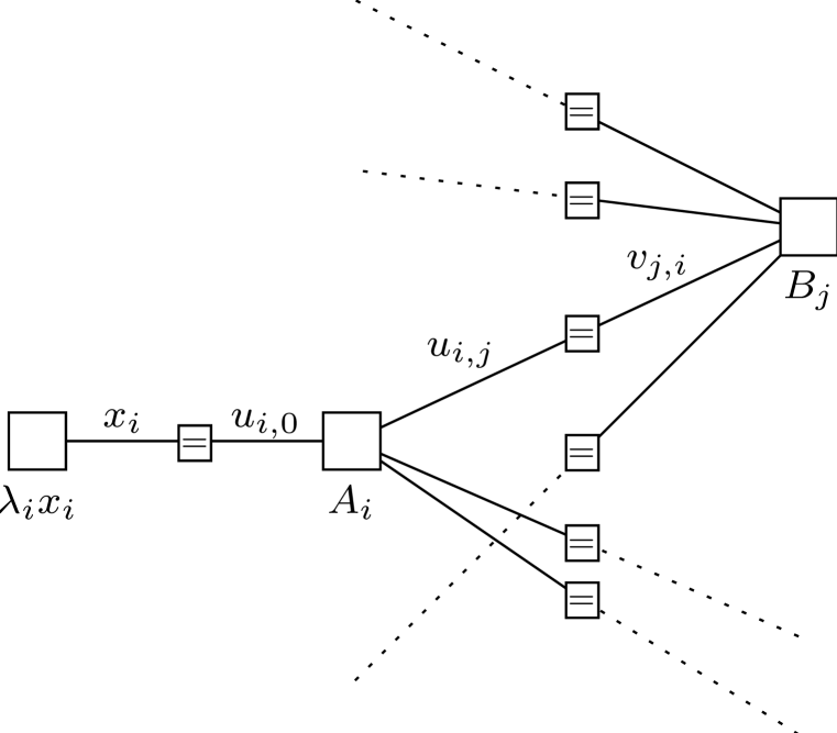
Figure 1: Representative part of the FFG for the augmented cost function in (1). (Note that this FFG has an additively written global function.)

The code $\mathcal{C}$ is used for data transmission over a binary-input memoryless channel with channel law $P_{\mathbf{Y}|\mathbf{X}}(\mathbf{y}|\mathbf{x})=\prod_{i\in\mathcal{I}}P_{Y|X}(y_{i}|x_{i})$. Upon observing $\mathbf{Y}=\mathbf{y}$, the maximum-likelihood decoding (MLD) rule decides for $\hat{\mathbf{x}}(\mathbf{y})=\arg\max_{\mathbf{x}\in\mathcal{C}}P_{\mathbf{Y}|\mathbf{X}}(\mathbf{y}|\mathbf{x})$. This can also be written as

MLD1: maximize $\displaystyle P_{\mathbf{Y}|\mathbf{X}}(\mathbf{y}|\mathbf{x})$ subject to $\displaystyle\mathbf{x}\in\mathcal{C}.$

It is clear that instead of $P_{\mathbf{Y}|\mathbf{X}}(\mathbf{y}|\mathbf{x})$ we can also maximize $\log P_{\mathbf{Y}|\mathbf{X}}(\mathbf{y}|\mathbf{x})=\sum_{i\in\mathcal{I}}\log P_{Y|X}(y_{i}|x_{i})$. Introducing $\lambda_{i}\triangleq\lambda_{i}(y_{i})\triangleq\log\bigl{(}\frac{P_{Y|X}(y_{i}|0)}{P_{Y|X}(y_{i}|1)}\bigr{)}$, $i\in\mathcal{I}$, and noting that $\log P_{Y|X}(y_{i}|x_{i})=-\lambda_{i}x_{i}+\log P_{Y|X}(y_{i}|0),\textbf{MLD1}$ can then be rewritten to read

MLD2: minimize $\displaystyle\sum_{i\in\mathcal{I}}\lambda_{i}x_{i}$ subject to $\displaystyle\mathbf{x}\in\mathcal{C}.$

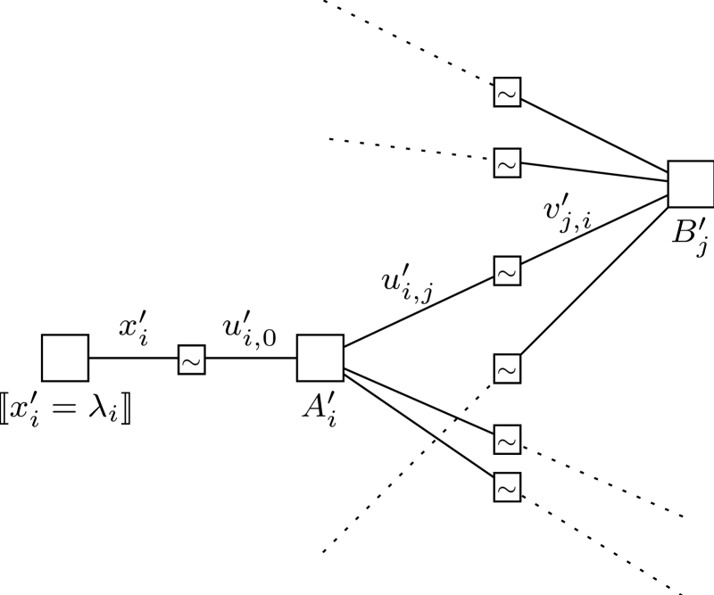
Figure 2: Representative part of the FFG for the augmented cost function in (2). Function nodes with a tilde sign in them mean the following: if such a function node is connected to edges $u$ and $v$ then the function value is $-\llbracket u=-v\rrbracket$. (Note that this FFG has an additively written global function.)

Because the cost function is linear, and a linear function attains its minimum at the extremal points of a convex set, this is essentially equivalent to

MLD3: minimize $\displaystyle\sum_{i\in\mathcal{I}}\lambda_{i}x_{i}$ subject to $\displaystyle\mathbf{x}\in\operatorname{conv}(\mathcal{C}).$

Although this is a linear program, it can usually not be solved efficiently because its description complexity is usually exponential in the block length of the code.

However, one might try to solve a relaxation of MLD3. Noting that $\operatorname{conv}(\mathcal{C})\subseteq\operatorname{conv}(\mathcal{C}_{1})\cap\cdots\cap\operatorname{conv}(\mathcal{C}_{m})$ (which follows from the fact that $\mathcal{C}=\mathcal{C}_{1}\cap\cdots\cap\mathcal{C}_{m}$), Feldman, Wainwright, and Karger [1, 2] defined the (primal) linear programming decoder (PLPD) to be given by the solution of the linear program

PLPD1: minimize $\displaystyle\sum_{i\in\mathcal{I}}\lambda_{i}x_{i}$ subject to $\displaystyle\mathbf{x}\in\operatorname{conv}(\mathcal{C}_{j})\ (j\in\mathcal{J}).$

The inequalities that are implied by the expression $\mathbf{x}\in\operatorname{conv}(\mathcal{C}_{j})$ can be found in [1, 2, 3, 4]. Although PLPD1 is usually suboptimal compared to MLD, it is especially attractive for LDPC codes for two reasons: firstly, for these codes the description complexities of $\operatorname{conv}(\mathcal{C}_{j})$, $j\in\mathcal{J}$, turn out to be low [2, 4] and, secondly, the relaxation is relatively benign only if the weight of the parity checks is low. There are many ways of reformulating this PLPD1 rule by introducing auxiliary variables: one way that we found particularly useful is shown as PLPD2 below. The reason for its usefulness is that there is a one-to-one correspondence between parts of the program and the FFG shown in Fig. 1, as we will discuss later on. Indeed, while the notation may seem heavy at first glance, it precisely reflects the structure of the constraints that are summarily folded into the seemingly simpler constraint $\mathbf{x}\in\operatorname{conv}(\mathcal{C}_{j})\ (j\in\mathcal{J})$ of PLPD1.

PLPD2: min. $\displaystyle\sum_{i\in\mathcal{I}}\lambda_{i}x_{i}$ subj. to $\displaystyle x_{i}$ $\displaystyle=u_{i,0}\quad$ $\displaystyle(i\in\mathcal{I}),$ $\displaystyle u_{i,j}$ $\displaystyle=v_{j,i}\quad$ $\displaystyle((i,j)\in\mathcal{E}),$ $\displaystyle\sum_{\mathbf{a}_{i}\in\mathcal{A}_{i}}\alpha_{i,\mathbf{a}_{i}}\mathbf{a}_{i}$ $\displaystyle=\mathbf{u}_{i}\quad$ $\displaystyle(i\in\mathcal{I}),$ $\displaystyle\sum_{\mathbf{b}_{j}\in\mathcal{B}_{j}}\beta_{j,\mathbf{b}_{j}}\mathbf{b}_{j}$ $\displaystyle=\mathbf{v}_{j}\quad$ $\displaystyle(j\in\mathcal{J}),$ $\displaystyle\alpha_{i,\mathbf{a}_{i}}$ $\displaystyle\geq 0\quad$ $\displaystyle(i\in\mathcal{I},\mathbf{a}_{i}\in\mathcal{A}_{i}),$ $\displaystyle\beta_{j,\mathbf{b}_{j}}$ $\displaystyle\geq 0\quad$ $\displaystyle(j\in\mathcal{J},\mathbf{b}_{j}\in\mathcal{B}_{j}),$ $\displaystyle\sum_{\mathbf{a}_{i}\in\mathcal{A}_{i}}\alpha_{i,\mathbf{a}_{i}}$ $\displaystyle=1\quad$ $\displaystyle(i\in\mathcal{I}),$ $\displaystyle\sum_{\mathbf{b}_{j}\in\mathcal{B}_{j}}\beta_{j,\mathbf{b}_{j}}$ $\displaystyle=1\quad$ $\displaystyle(j\in\mathcal{J}).$

Here we used the following codes, variables and vectors. The code $\mathcal{A}_{i}\subseteq\{0,1\}^{|\{0\}\cup\mathcal{J}_{i}|}$, $i\in\mathcal{I}$, is the set containing the all-zeros vector and the all-ones vector of length $|\mathcal{J}_{i}|+1$, and $\mathcal{B}_{j}\subseteq\{0,1\}^{|\mathcal{I}_{j}|}$, $j\in\mathcal{J}$, is the code $\mathcal{C}_{j}$ shortened at the positions $\mathcal{I}\setminus\mathcal{I}_{j}$. For $i\in\mathcal{I}$ we will also use the vectors $\mathbf{u}_{i}$ where the entries are indexed by $\{0\}\cup\mathcal{J}_{i}$ and denoted by $u_{i,j}\triangleq[\mathbf{u}_{i}]_{j}$, and for $j\in\mathcal{J}$ we will use the vectors $\mathbf{v}_{j}$ where the entries are indexed by $\mathcal{I}_{j}$ and denoted by $v_{j,i}\triangleq[\mathbf{v}_{j}]_{i}$. Later on, we will use a similar notation for the entries of $\mathbf{a}_{i}$ and $\mathbf{b}_{j}$, i.e. we will use $a_{i,j}\triangleq[\mathbf{a}_{i}]_{j}$ and $b_{j,i}\triangleq[\mathbf{b}_{j}]_{i}$, respectively.

The above optimization problem is elegantly represented by the FFG shown in Fig. 1. In order to express the LP itself in an FFG we have to express the constraints as additive cost terms. This is easily accomplished by assigning the cost $+\infty$ to any configuration of variables that does not satisfy the LP constraints. The above minimization problem is then equivalent to the (unconstrained) minimization of the augmented cost function

$$\sum_{i\in\mathcal{I}}\lambda_{i}x_{i} +\sum_{i\in\mathcal{I}}\big{\llbracket}x_{i}=u_{i,0}\big{\rrbracket}+\sum_{(i,j)\in\mathcal{E}}\big{\llbracket}u_{i,j}=v_{j,i}\big{\rrbracket}$$

$$+\sum_{i\in\mathcal{I}}A_{i}(\mathbf{u}_{i})+\sum_{j\in\mathcal{J}}B_{j}(\mathbf{v}_{j}),$$ (1)

where for all $i\in\mathcal{I}$ and all $j\in\mathcal{J}$, respectively, we introduced

$$A_{i}(\mathbf{u}_{i}) \triangleq\left\llbracket\sum_{\mathbf{a}_{i}\in\mathcal{A}_{i}}\alpha_{i,\mathbf{a}_{i}}\mathbf{a}_{i}=\mathbf{u}_{i}\right\rrbracket$$

$$\quad\quad+\sum_{\mathbf{a}_{i}\in\mathcal{A}_{i}}\big{\llbracket}\alpha_{i,\mathbf{a}_{i}}\geq 0\big{\rrbracket}+\left\llbracket\sum_{\mathbf{a}_{i}\in\mathcal{A}_{i}}\alpha_{i,\mathbf{a}_{i}}=1\right\rrbracket,$$

$$B_{j}(\mathbf{v}_{j}) \triangleq\left\llbracket\sum_{\mathbf{b}_{j}\in\mathcal{B}_{j}}\beta_{j,\mathbf{b}_{j}}\mathbf{b}_{j}=\mathbf{v}_{j}\right\rrbracket$$

$$\quad\quad+\sum_{\mathbf{b}_{j}\in\mathcal{B}_{j}}\big{\llbracket}\beta_{j,\mathbf{b}_{j}}\geq 0\big{\rrbracket}+\left\llbracket\sum_{\mathbf{b}_{j}\in\mathcal{B}_{j}}\beta_{j,\mathbf{b}_{j}}=1\right\rrbracket.$$

With this, the global function of the FFG in Fig. 1 equals the augmented cost function in (1) and we have represented the LP in terms of an FFG.

Of course, any reader who is familiar with LDPC codes will have no problem to make a connection between the FFG of Fig. 1 and the standard representation as a Tanner graph. Indeed, a node $A_{i}$ corresponds to a variable node in a Tanner graph and a node $B_{j}$ takes over the role of a parity check node. However, instead of simply assigning a variable to node $A_{i}$ we assign a local set of constraints corresponding to the convex hull of a repetition code. These are the equations $\sum_{\mathbf{a}_{i}\in{\cal{A}}_{i}}\alpha_{i,\mathbf{a}_{i}}\mathbf{a}_{i}=\mathbf{u}_{i}$, $\alpha_{i,\mathbf{a}_{i}}\geq 0$, $\sum_{\mathbf{a}_{i}\in{\cal{A}}_{i}}\alpha_{i,\mathbf{a}_{i}}=1$. Similarly, the equations for the convex hull of a simple parity-check code can be identified for nodes $B_{j}$.

III The Dual Linear Program

The dual linear program [14] of PLPD2 is

DLPD2: max. $\displaystyle\sum_{i\in\mathcal{I}}\phi^{\prime}_{i}$ $\displaystyle+\sum_{j\in\mathcal{J}}\theta^{\prime}_{j}$ subj. to $\displaystyle\phi^{\prime}_{i}$ $\displaystyle\leq\min_{\mathbf{a}_{i}\in\mathcal{A}_{i}}\langle-\mathbf{u}^{\prime}_{i},\mathbf{a}_{i}\rangle\quad$ $\displaystyle(i\in\mathcal{I}),$ $\displaystyle\theta^{\prime}_{j}$ $\displaystyle\leq\min_{\mathbf{b}_{j}\in\mathcal{B}_{j}}\langle-\mathbf{v}^{\prime}_{j},\mathbf{b}_{j}\rangle\quad$ $\displaystyle(j\in\mathcal{J}),$ $\displaystyle u^{\prime}_{i,j}$ $\displaystyle=-v^{\prime}_{j,i}\quad$ $\displaystyle((i,j)\in\mathcal{E}),$ $\displaystyle u^{\prime}_{i,0}$ $\displaystyle=-x^{\prime}_{i}\quad$ $\displaystyle(i\in\mathcal{I}),$ $\displaystyle x^{\prime}_{i}$ $\displaystyle=\lambda_{i}\quad$ $\displaystyle(i\in\mathcal{I}).$

Expressing the constraints as additive cost terms, the above maximization problem is equivalent to the (unconstrained) maximization of the augmented cost function

$$\sum_{i\in\mathcal{I}}A^{\prime}_{i}(\mathbf{u}^{\prime}_{i})+\sum_{j\in\mathcal{J}}B^{\prime}_{j}(\mathbf{v}^{\prime}_{j})-\sum_{(i,j)\in\mathcal{E}}\llbracket u^{\prime}_{i,j}=-v^{\prime}_{j,i}\rrbracket$$

$$-\sum_{i\in\mathcal{I}}\llbracket u^{\prime}_{i,0}=-x^{\prime}_{i}\rrbracket-\sum_{i\in\mathcal{I}}\llbracket x^{\prime}_{i}=\lambda_{i}\rrbracket,$$ (2)

with

$$A^{\prime}_{i}(\mathbf{u}^{\prime}_{i}) =\phi^{\prime}_{i}-\left\llbracket\phi^{\prime}_{i}\leq\min_{\mathbf{a}_{i}\in\mathcal{A}_{i}}\langle-\mathbf{u}^{\prime}_{i},\mathbf{a}_{i}\rangle\right\rrbracket,$$

$$B^{\prime}_{j}(\mathbf{v}^{\prime}_{j}) =\theta^{\prime}_{j}-\left\llbracket\theta^{\prime}_{j}\leq\min_{\mathbf{b}_{j}\in\mathcal{B}_{j}}\langle-\mathbf{v}^{\prime}_{j},\mathbf{b}_{j}\rangle\right\rrbracket.$$

The augmented cost function in (2) is represented by the FFG in Fig. 2. (For deriving DLPD2 we used the techniques introduced in [15, 16]; note that the techniques presented there can also be used to systematically derive the dual function of much more complicated functions that are sums of convex functions. Alternatively, one might also use results from monotropic programming, cf. e.g. [17].)

Because for each $i\in\mathcal{I}$ the variable $\phi^{\prime}_{i}$ is involved in only one inequality, the optimal solution does not change if we replace the corresponding inequality signs by equality signs in DLPD2. The same comment holds for all $\theta^{\prime}_{j}$, $j\in\mathcal{J}$.

Definition 1

Let $\mathcal{A}\triangleq\mathcal{A}_{1}\times\cdots\times\mathcal{A}_{n}$ and let $\mathcal{B}\triangleq\mathcal{B}_{1}\times\cdots\times\mathcal{B}_{m}$. For $\mathbf{a}\triangleq(\mathbf{a}_{1},\ldots,\mathbf{a}_{n})\in\mathcal{A}$ and $\mathbf{b}\triangleq(\mathbf{b}_{1},\ldots,\mathbf{b}_{m})\in\mathcal{B}$ define

$$g^{\prime}_{\mathbf{a},\mathbf{b}}(\mathbf{u}^{\prime}) \triangleq\sum_{i\in\mathcal{I}}\langle-\mathbf{u}^{\prime}_{i},\mathbf{a}_{i}\rangle+\sum_{j\in\mathcal{J}}\langle+\mathbf{u}^{\prime}_{j},\mathbf{b}_{j}\rangle,$$

where, with a slight abuse of notation, $\mathbf{u}^{\prime}_{j}$ is such that $[\mathbf{u}^{\prime}_{j}]_{i}=u^{\prime}_{i,j}$ for all $(i,j)\in\mathcal{E}$. Moreover, we call $(\mathbf{a},\mathbf{b})\in\mathcal{A}\times\mathcal{B}$ consistent if $a_{i,j}=b_{j,i}$ for all $(i,j)\in\mathcal{E}$. $\square$

Obviously, $g^{\prime}_{\mathbf{a},\mathbf{b}}(\mathbf{u}^{\prime})$ is a linear function in $\mathbf{u}^{\prime}$. With the above definition, DLPD2 can be rewritten to read

DLPD3: max. $\displaystyle g^{\prime}_{\mathbf{a},\mathbf{b}}(\mathbf{u}^{\prime})$ subj. to $\displaystyle(\mathbf{a},\mathbf{b})\in\mathcal{A}\times\mathcal{B},$ $\displaystyle u^{\prime}_{i,0}=-\lambda_{i}$ $\displaystyle\quad(i\in\mathcal{I}).$

Lemma 2

Let $\mathbf{u}^{\prime}$ be such that $u^{\prime}_{i,0}=-\lambda_{i}$, $i\in\mathcal{I}$. If $(\mathbf{a},\mathbf{b})\in\mathcal{A}\times\mathcal{B}$ is consistent then $g^{\prime}_{\mathbf{a},\mathbf{b}}(\mathbf{u}^{\prime})$ is constant in $\mathbf{u}^{\prime}$. Moreover, $g^{\prime}_{\mathbf{a},\mathbf{b}}(\mathbf{u}^{\prime})=\langle\boldsymbol{\lambda},\mathbf{x}\rangle$, where $\mathbf{x}$ is such that $x_{i}=a_{i,0}$, $i\in\mathcal{I}$. If $(\mathbf{a},\mathbf{b})\in\mathcal{A}\times\mathcal{B}$ is not consistent then $g^{\prime}_{\mathbf{a},\mathbf{b}}(\mathbf{u}^{\prime})$ is not a constant function for at least one $u_{i,j}$, $(i,j)\in\mathcal{E}$.

Proof: See Sec. -A. $\square$

IV A Softened Dual Linear Program

For any $\kappa\in\mathbb{R}_{++}$, we define the soft-minimum operator to be

$${\min_{\ell}}^{(\kappa)}z_{\ell} \triangleq-\frac{1}{\kappa}\log\left(\sum_{\ell}\mathrm{e}^{-\kappa z_{\ell}}\right).$$

(Note that $\kappa$ can be given the interpretation of an inverse temperature.) One can easily check that ${\min_{\ell}}^{(\kappa)}z_{\ell}\leq\min_{\ell}\{z_{\ell}\}$ with equality in the limit $\kappa\to+\infty$. Replacing the minimum operators in DLPD2 by soft-minimum operators, we obtain the modified optimization problem

SDLPD2: max. $\displaystyle\sum_{i\in\mathcal{I}}\phi^{\prime}_{i}$ $\displaystyle+\sum_{j\in\mathcal{J}}\theta^{\prime}_{j}$ subj. to $\displaystyle\phi^{\prime}_{i}$ $\displaystyle\leq{\min_{\mathbf{a}_{i}\in\mathcal{A}_{i}}}^{(\kappa_{i})}\langle-\mathbf{u}^{\prime}_{i},\mathbf{a}_{i}\rangle\$ $\displaystyle(i\in\mathcal{I}),$ $\displaystyle\theta^{\prime}_{j}$ $\displaystyle\leq{\min_{\mathbf{b}_{j}\in\mathcal{B}_{j}}}^{(\kappa_{j})}\langle-\mathbf{v}^{\prime}_{j},\mathbf{b}_{j}\rangle\$ $\displaystyle(j\in\mathcal{J}),$ $\displaystyle u^{\prime}_{i,j}$ $\displaystyle=-v^{\prime}_{j,i}\quad$ $\displaystyle((i,j)\in\mathcal{E}),$ $\displaystyle u^{\prime}_{i,0}$ $\displaystyle=-x^{\prime}_{i}\quad$ $\displaystyle(i\in\mathcal{I}),$ $\displaystyle x^{\prime}_{i}$ $\displaystyle=\lambda_{i}\quad$ $\displaystyle(i\in\mathcal{I}).$

In the following, unless noted otherwise, we will set $\kappa_{i}\triangleq\kappa$, $i\in\mathcal{I}$, and $\kappa_{j}\triangleq\kappa$, $j\in\mathcal{J}$, for some $\kappa\in\mathbb{R}_{++}$. It is clear that in the limit $\kappa\to+\infty$ we recover DLPD2.

V A Comment on the Dual of the Softened Dual Linear Program

Let

$$H(\alpha_{i}) \triangleq-\sum_{\mathbf{a}_{i}\in\mathcal{A}_{i}}\alpha_{i,\mathbf{a}_{i}}\log(\alpha_{i,\mathbf{a}_{i}})$$

be the entropy of of a random variable whose pmf takes on the values $\{\alpha_{i,\mathbf{a}_{i}}\}_{\mathbf{a}_{i}\in\mathcal{A}_{i}}$. Similarly, let

$$H(\beta_{j}) \triangleq-\sum_{\mathbf{b}_{j}\in\mathcal{B}_{j}}\beta_{j,\mathbf{b}_{j}}\log(\beta_{j,\mathbf{b}_{j}}).$$

The dual of SDLDP2 can then be written as

DSLPD2: min. $\displaystyle\sum_{i\in\mathcal{I}}\lambda_{i}x_{i}-\frac{1}{\kappa}\sum_{i\in\mathcal{I}}H(\alpha_{i})-\frac{1}{\kappa}\sum_{j\in\mathcal{J}}H(\beta_{j})$ subj. to $\displaystyle\text{the same constraints as in {PLPD2}}.$

We note that this is very close to the following Bethe free energy optimization problem, cf. e.g. [18]

BFE1: min. $\displaystyle\sum_{i\in\mathcal{I}}\lambda_{i}x_{i}$ $\displaystyle+\frac{1}{\kappa}\sum_{i\in\mathcal{I}}(|\mathcal{J}_{i}|-1)H(\alpha_{i})-\frac{1}{\kappa}\sum_{j\in\mathcal{J}}H(\beta_{j})$ subj. to $\displaystyle\text{the same constraints as in {PLPD2}},$

which, in turn, can also be written as

BFE2: min. $\displaystyle\sum_{i\in\mathcal{I}}\lambda_{i}x_{i}-\frac{1}{\kappa}\sum_{i\in\mathcal{I}}H(\alpha_{i})-\sum_{j\in\mathcal{J}}H(\beta_{j})$ $\displaystyle+\frac{1}{\kappa}\sum_{i\in\mathcal{I}}|\mathcal{J}_{i}|H(\alpha_{i})$ subj. to $\displaystyle\text{the same constraints as in {PLPD2}}.$

Without going into the details we note that the term $+\frac{1}{\kappa}\sum_{i\in\mathcal{I}}(|\mathcal{J}_{i}|-1)H(\alpha_{i})$ is responsible for the fact that the cost function in BFE2 is usually non-convex for FFGs with cycles.

VI Decoding Algorithm 1

In the following, we assume that $u^{\prime}_{i,j}$ and $v^{\prime}_{j,i}$ are “coupled”, i.e. we always have $u^{\prime}_{i,j}=-v^{\prime}_{j,i}$ for all $(i,j)\in\mathcal{E}$.

The first algorithm that we propose is a coordinate-ascent-type algorithm for solving SDLPD2. The main idea is to select edges $(i,j)\in\mathcal{E}$ according to some update schedule: for each selected edge $(i,j)\in\mathcal{E}$ we then replace the old values of $u^{\prime}_{i,j}$, $\phi^{\prime}_{i}$, and $\theta^{\prime}_{j}$ by new values such that the dual cost function is increased (or at least not decreased). Practically, this means that we have to find an $\overline{u}^{\prime}_{i,j}$ such that $h^{\prime}(\overline{u}^{\prime}_{i,j})\geq h^{\prime}(u^{\prime}_{i,j})$, where

$$h^{\prime}(u^{\prime}_{i,j}) \triangleq{\min_{\mathbf{a}_{i}\in\mathcal{A}_{i}}}^{(\kappa)}\langle-\mathbf{u}^{\prime}_{i},\mathbf{a}_{i}\rangle+{\min_{\mathbf{b}_{j}\in\mathcal{B}_{j}}}^{(\kappa)}\langle-\mathbf{v}^{\prime}_{j},\mathbf{b}_{j}\rangle.$$

A simple way to achieve this is by setting

$$\overline{u}^{\prime}_{i,j} \triangleq\arg\max_{u^{\prime}_{i,j}}h^{\prime}(u^{\prime}_{i,j}).$$ (3)

The variables $\phi^{\prime}_{i}$ and $\theta^{\prime}_{j}$ are then updated accordingly so that we obtain a new (dual) feasible point.

Lemma 3

The value of $\overline{u}^{\prime}_{i,j}$ in (3) is given by

$$\overline{u}^{\prime}_{i,j} =\frac{1}{2}\bigg{(}+\big{(}S^{\prime}_{i,0}-S^{\prime}_{i,1}\big{)}-\big{(}T^{\prime}_{j,0}-T^{\prime}_{j,1}\big{)}\bigg{)},$$

where

$$S^{\prime}_{i,0} \triangleq-{\min_{\mathbf{a}_{i}\in\mathcal{A}_{i}\atop a_{i,j}=0}}^{(\kappa)}\langle-\tilde{\mathbf{u}}_{i},\tilde{\mathbf{a}}_{i}\rangle,$$

$$S^{\prime}_{i,1} \triangleq-{\min_{\mathbf{a}_{i}\in\mathcal{A}_{i}\atop a_{i,j}=1}}^{(\kappa)}\langle-\tilde{\mathbf{u}}_{i},\tilde{\mathbf{a}}_{i}\rangle,$$

$$T^{\prime}_{j,0} \triangleq-{\min_{\mathbf{b}_{j}\in\mathcal{B}_{j}\atop b_{j,i}=0}}^{(\kappa)}\langle-\tilde{\mathbf{v}}_{j},\tilde{\mathbf{b}}_{j}\rangle,$$

$$T^{\prime}_{j,1} \triangleq-{\min_{\mathbf{b}_{j}\in\mathcal{B}_{j}\atop b_{j,i}=1}}^{(\kappa)}\langle-\tilde{\mathbf{v}}_{j},\tilde{\mathbf{b}}_{j}\rangle.$$

Here the vectors $\tilde{\mathbf{u}}$ and $\tilde{\mathbf{a}}$ are the vectors $\mathbf{u}$ and $\mathbf{a}$, respectively, where the $j$-th position has been omitted. Similarly, the vectors $\tilde{\mathbf{v}}$ and $\tilde{\mathbf{b}}$ are the vectors $\mathbf{v}$ and $\mathbf{b}$, respectively, where the $i$-th position has been omitted. Note that the differences $S^{\prime}_{i,0}-S^{\prime}_{i,1}$ and $T^{\prime}_{i,0}-T^{\prime}_{i,1}$, which are required for computing $\overline{u}^{\prime}_{i,j}$, can be obtained very efficiently by using the sum-product algorithm [11].

Proof: See Sec. -B. $\square$

In the introduction we wrote that we would like to use the special structure of the primal/dual LP at hand; Lemma 3 is a first example how this can be done. Please note that when computing the necessary quantities (for the case $\kappa=1$) one has do computations that are (up to some flipped signs) equivalent to computations that are done during message updates while performing sum-product algorithm decoding of the LDPC code at hand.

Lemma 4

Assume that all the rows of the parity-check matrix $\mathbf{H}$ of the code $\mathcal{C}$ have Hamming weight at least $3$. Then, updating cyclically all edges $(i,j)\in\mathcal{E}$, the above coordinate-ascent algorithm converges to the maximum of SDLPD2.

Proof: See Sec. -C $\square$

As we mentioned in the proof of Lemma 4, the above algorithm can be seen as a Gauss-Seidel-type algorithm. Let us remark that there are ways to see sum-product algorithm decoding as applying a Gauss-Seidel-type algorithm to the dual of the Bethe free energy, see e.g. [19, 20]; in light of the observations in Sec. V it is not surprising that there is a tight relationship between our algorithms and the above-mentioned algorithms.

Lemma 5

For $\kappa\to\infty$, the function $h^{\prime}(u^{\prime}_{i,j})$ is maximized by any value $u^{\prime}_{i,j}$ that lies in the closed interval between

$$\big{(}S^{\prime}_{i,0}-S^{\prime}_{i,1}\big{)}\quad\text{ and }\quad-\big{(}T^{\prime}_{j,0}-T^{\prime}_{j,1}\big{)},$$

where

$$S^{\prime}_{i,0} \triangleq-\min_{\mathbf{a}_{i}\in\mathcal{A}_{i}\atop a_{i,j}=0}\langle-\tilde{\mathbf{u}}_{i},\tilde{\mathbf{a}}_{i}\rangle,$$

$$S^{\prime}_{i,1} \triangleq-\min_{\mathbf{a}_{i}\in\mathcal{A}_{i}\atop a_{i,j}=1}\langle-\tilde{\mathbf{u}}_{i},\tilde{\mathbf{a}}_{i}\rangle,$$

$$T^{\prime}_{j,0} \triangleq-\min_{\mathbf{b}_{j}\in\mathcal{B}_{j}\atop b_{j,i}=0}\langle-\tilde{\mathbf{v}}_{j},\tilde{\mathbf{b}}_{j}\rangle,$$

$$T^{\prime}_{j,1} \triangleq-\min_{\mathbf{b}_{j}\in\mathcal{B}_{j}\atop b_{j,i}=1}\langle-\tilde{\mathbf{v}}_{j},\tilde{\mathbf{b}}_{j}\rangle.$$

Proof: See Sec. -D. $\square$

Conjecture 6

Again, we can cyclically update the edges $(i,j)\in\mathcal{E}$ whereby the new $\overline{u}^{\prime}_{i,j}$ is chosen randomly in the above interval. Although the objective function for $\kappa\to+\infty$ is concave, it is not everywhere differentiable. This makes a convergence proof in the style of Lemma 4 difficult. We think that we can again use the special structure of the LP at hand to show that the algorithm cannot get stuck at a suboptimal point. However, so far we do not have a proof of this fact. Sec. -E discusses briefly why a convergence proof is not a trivial extension of Lemma 4. $\square$

Before ending this section, let us briefly remark how a codeword decision is obtained from a solution of DLPD2. Assume that $\hat{\mathbf{x}}$ is the pseudo-codeword that is the solution to PLPD1 or to PLPD2. Knowing the solution of DLPD2 we cannot directly find $\hat{\mathbf{x}}$, however, we can find out at what positions $\hat{\mathbf{x}}$ is $0$ and at what positions $\hat{\mathbf{x}}$ is $1$. Namely, letting $\check{\mathbf{x}}\in\{0,?,1\}^{n}$ have the components

$$\check{x}_{i}\triangleq\begin{cases}0&\text{ if }\langle-\mathbf{u}^{\prime}_{i},\mathbf{a}_{i}\rangle|_{\mathbf{a}_{i}=\mathbf{0}}\ <\ \langle-\mathbf{u}^{\prime}_{i},\mathbf{a}_{i}\rangle|_{\mathbf{a}_{i}=\mathbf{1}}\\ ?&\text{ if }\langle-\mathbf{u}^{\prime}_{i},\mathbf{a}_{i}\rangle|_{\mathbf{a}_{i}=\mathbf{0}}\ =\ \langle-\mathbf{u}^{\prime}_{i},\mathbf{a}_{i}\rangle|_{\mathbf{a}_{i}=\mathbf{1}}\\ 1&\text{ if }\langle-\mathbf{u}^{\prime}_{i},\mathbf{a}_{i}\rangle|_{\mathbf{a}_{i}=\mathbf{0}}\ >\ \langle-\mathbf{u}^{\prime}_{i},\mathbf{a}_{i}\rangle|_{\mathbf{a}_{i}=\mathbf{1}}\end{cases},$$

we have $\check{x}_{i}=\hat{x}_{i}$ when $\hat{x}_{i}$ equals $0$ or $1$ and $\check{x}_{i}=\ ?$ when $\hat{x}_{i}\in(0,1)$. In other words, with the solution to DLPD2 we do not get the exact $\hat{\mathbf{x}}$ in case $\hat{\mathbf{x}}$ is not a codeword. However, as a side remark, because $\operatorname{supp}(\hat{\mathbf{x}})=\operatorname{supp}(\check{\mathbf{x}})$ (where $\operatorname{supp}$ is the set of all non-zero positions) we can use $\check{\mathbf{x}}$ to find the stopping set [21] associated to $\hat{\mathbf{x}}$.

VII Decoding Algorithm 2

Again, we assume that $u^{\prime}_{i,j}$ and $v^{\prime}_{j,i}$ are “coupled”, i.e. we always have $u^{\prime}_{j,i}=-v^{\prime}_{i,j}$ for all $(i,j)\in\mathcal{E}$.

While the iterative solutions of the coordinate-ascent methods that we presented in the previous section resemble the traditional min-sum algorithm decoding rules (and sum-product algorithm decoding rules) relatively closely, other methods for solving the linear program also offer attractive complexity/performance trade-offs. We would like to point out one such algorithm which is well suited for the linear programming problem arising from the decoding setup. Indeed, observing the formulation of the dual linear program DLPD2, sub-gradient methods are readily available to perform the required maximization. However, in order to exploit the structure of the problem we focus our attention to incremental sub-gradient methods [22]. Algorithms belonging to this family of optimization procedures allow us to exploit the fact that the objective function is a sum of a number of terms and we can operate on each term, i.e. each constituent code in the FFG, individually. In order to derive a concise formulation of the procedure we start by considering a check node $j\in\mathcal{J}$. For a particular choice of dual variables $\mathbf{v}^{\prime}_{j}$ the contribution of node $j$ to the overall objective function is

$$f^{\prime}_{j}(\mathbf{v}^{\prime}_{j}) =\min_{\mathbf{b}_{j}\in\mathcal{B}_{j}}\langle-\mathbf{v}^{\prime}_{j},\mathbf{b}_{j}\rangle.$$

Let a function $\mathbf{g}^{\prime}(\mathbf{v}^{\prime}_{j})$ be defined as $\mathbf{g}^{\prime}_{j}(\mathbf{v}^{\prime}_{j})\triangleq-\arg\min_{\mathbf{b}_{j}\in\mathcal{B}_{j}}\langle-\mathbf{v}^{\prime}_{j},\mathbf{b}_{j}\rangle$ where, if ambiguities exist, $\mathbf{g}^{\prime}_{j}(\mathbf{v}^{\prime}_{j})$ is the negative of an arbitrary combination of the set of ambiguous vectors $\mathbf{b}^{\prime}_{j}$. Note that for obtaining $\mathbf{g}^{\prime}_{j}(\mathbf{v}^{\prime}_{j})$ we can again take advantage of the special structure of the LP at hand.

Using the defining property of sub-gradient $\mathbf{d}^{\prime}_{j}$ at $\mathbf{v}^{\prime}_{j}$, namely,

$$f^{\prime}(\mathbf{\breve{v}}^{\prime}_{j}) \leq f(\mathbf{v}^{\prime}_{j})+\langle\mathbf{d}^{\prime}_{j},\mathbf{\breve{v}}^{\prime}_{j}-\mathbf{v}^{\prime}_{j})$$

it can be seen that $\mathbf{g}^{\prime}_{j}(\mathbf{v}^{\prime}_{j})$ is a sub-gradient. We can then update $\mathbf{v}^{\prime}_{j}$ as follows:

$$\mathbf{v}^{\prime}_{j} \leftarrow\mathbf{v}^{\prime}_{j}+\mu_{\ell}\mathbf{g}^{\prime}_{j}(\mathbf{v}^{\prime}_{j}),$$

where $\mu_{\ell}\in\mathbb{R}_{++}$. Given this, one can formulate the following algorithm: at iteration $\ell$ update consecutively all check nodes $j\in\mathcal{J}$ and then, in an analogous manner, update all variable nodes $i\in\mathcal{I}$.

For this algorithm we cannot guarantee that the value of the objective function increases for each iteration (not even for small $\mu_{\ell}$). Nevertheless, its convergence to the maximum can be guaranteed for a suitably chosen sequence $\{\alpha_{\ell}\}_{\ell\geq 1}$ [22].

Let us point out that gradient-type methods have also been used to decode codes in different contexts, see e.g. the work by Lucas et al. [23]. However, the setup in [23] has some significant differences to the setup here: firstly, the objective function of the optimization problem in [23] does not depend on the observed log-liklihood ratio vector $\boldsymbol{\lambda}$, secondly, the starting point in [23] is chosen as a function of $\boldsymbol{\lambda}$.

VIII Simulation Results

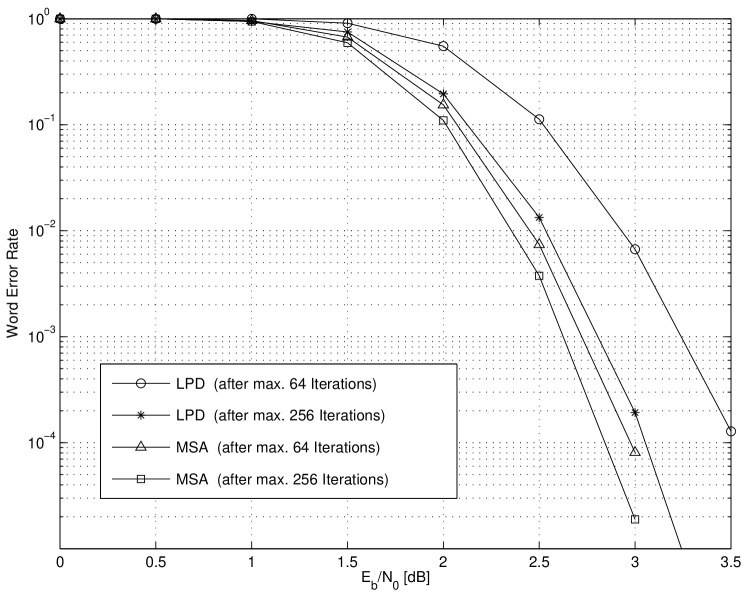
Figure 3: Decoding results for a $[1000,500]$ LDPC code. (See Sec. VIII for more details.)

As a proof of concept we show some simulation results for a randomly generated $(3,6)$-regular $[1000,500]$ LDPC code where four-cycles in the Tanner graph have been eliminated. Fig. 3 shows the decoding results based on Decoding Algorithm $1$ with update rule Lemma 5 compared with standard min-sum algorithm decoding [11].

IX Conclusions

We have discussed some initial steps towards algorithms that are specially targeted for efficiently solving the LP that appears in LP decoding. It has been shown that algorithms with memory and time complexity similar to min-sum algorithm decoding can be achieved. There are many avenues to pursue this topic further, e.g. by improving the update schedule, by studying how to design codes that allow efficient hardware implementation of the proposed algorithms, or by investigating other algorithms that use the structure of the LP that appears in LP decoding. We hope that this paper raises the interest in exploring these research directions.

Finally, without going into the details, let us remark that the algorithms here can also be used to solve certain linear programs whose value can be used to obtain lower bounds on the minimal AWGNC pseudo-weight of parity-check matrices, cf. [8, Claim 3]. (Actually, one does not really need to solve the linear program in [8, Claim 3] in order to obtain a lower bound on the minimum AWGNC pseudo-weight, any dual feasible point is good enough for that purpose.)

-A Proof of Lemma 2

If $(\mathbf{a},\mathbf{b})$ is consistent then

$$g^{\prime}_{\mathbf{a},\mathbf{b}}(\mathbf{u}^{\prime}) =\sum_{i\in\mathcal{I}}\langle-\mathbf{u}^{\prime}_{i},\mathbf{a}_{i}\rangle+\sum_{j\in\mathcal{J}}\langle+\mathbf{u}^{\prime}_{j},\mathbf{b}_{j}\rangle$$

$$=-\sum_{i\in\mathcal{I}}u^{\prime}_{i,0}a_{i,0}-\sum_{(i,j)\in\mathcal{E}}u^{\prime}_{i,j}a_{i,j}$$

$$\quad\,+\sum_{(i,j)\in\mathcal{E}}u^{\prime}_{i,j}b_{j,i}$$

$$=-\sum_{i\in\mathcal{I}}u^{\prime}_{i,0}a_{i,0}$$

$$=\sum_{i\in\mathcal{I}}\lambda_{i}x_{i}.$$

On the other hand, if $(\mathbf{a},\mathbf{b})$ is not consistent and $(i,j)\in\mathcal{E}$ is such that $a_{i,j}\neq b_{j,i}$ then $g^{\prime}_{\mathbf{a},\mathbf{b}}(\mathbf{u}^{\prime})$ is non-constant in $u^{\prime}_{i,j}$.

-B Proof of Lemma 3

This result is obtained by taking the derivative of $h^{\prime}(u^{\prime}_{i,j})$, setting it equal to zero, and solving for $u^{\prime}_{i,j}$. Let us go through this procedure step by step. Using the fact that $u^{\prime}_{i,j}=-v^{\prime}_{j,i}$, the function $h^{\prime}(u^{\prime}_{i,j})$ can be written as

$$h^{\prime}(u^{\prime}_{i,j}) \triangleq{\min_{\mathbf{a}_{i}\in\mathcal{A}_{i}}}^{(\kappa)}\langle-\mathbf{u}^{\prime}_{i},\mathbf{a}_{i}\rangle+{\min_{\mathbf{b}_{j}\in\mathcal{B}_{j}}}^{(\kappa)}\langle-\mathbf{v}^{\prime}_{j},\mathbf{b}_{j}\rangle$$

$$=-\frac{1}{\kappa}\log\left(\sum_{\mathbf{a}_{i}\in\mathcal{A}_{i}}\mathrm{e}^{+\kappa\langle\mathbf{u}_{i},\mathbf{a}_{i}\rangle}\right)$$

$$\quad\,-\frac{1}{\kappa}\log\left(\sum_{\mathbf{b}_{j}\in\mathcal{B}_{j}}\mathrm{e}^{+\kappa\langle\mathbf{v}_{j},\mathbf{b}_{j}\rangle}\right)$$

$$=-\frac{1}{\kappa}\log\left(\sum_{\mathbf{a}_{i}\in\mathcal{A}_{i}}\mathrm{e}^{+\kappa u_{i,j}a_{i,j}+\kappa\langle\tilde{\mathbf{u}}_{i},\tilde{\mathbf{a}}_{i}\rangle}\right)$$

$$\quad\,-\frac{1}{\kappa}\log\left(\sum_{\mathbf{b}_{j}\in\mathcal{B}_{j}}\mathrm{e}^{-\kappa u_{i,j}b_{j,i}+\kappa\langle\tilde{\mathbf{v}}_{j},\tilde{\mathbf{b}}_{j}\rangle}\right)$$

$$=-\frac{1}{\kappa}\log\left(\mathrm{e}^{\kappa S^{\prime}_{i,0}}+\mathrm{e}^{+\kappa u^{\prime}_{i,j}}\mathrm{e}^{\kappa S^{\prime}_{i,1}}\right)$$

$$\quad\,-\frac{1}{\kappa}\log\left(\mathrm{e}^{\kappa T^{\prime}_{j,0}}+\mathrm{e}^{-\kappa u^{\prime}_{i,j}}\mathrm{e}^{\kappa T^{\prime}_{j,1}}\right)$$

Setting the derivative of $h^{\prime}(u^{\prime}_{i,j})$ with respect to $u^{\prime}_{i,j}$ equal to zero we obtain

$$0 \overset{!}{=}\frac{\partial h^{\prime}(u^{\prime}_{i,j})}{\partial u^{\prime}_{i,j}}$$

$$=-\frac{1}{\kappa}\cdot\frac{+\kappa\mathrm{e}^{+\kappa u^{\prime}_{i,j}}\mathrm{e}^{\kappa S^{\prime}_{i,1}}}{\mathrm{e}^{\kappa S^{\prime}_{i,0}}+\mathrm{e}^{+\kappa u^{\prime}_{i,j}}\mathrm{e}^{\kappa S^{\prime}_{i,1}}}$$

$$\quad\,-\frac{1}{\kappa}\cdot\frac{-\kappa\mathrm{e}^{-\kappa u^{\prime}_{i,j}}\mathrm{e}^{\kappa T^{\prime}_{j,1}}}{\mathrm{e}^{\kappa T^{\prime}_{j,0}}+\mathrm{e}^{-\kappa u^{\prime}_{i,j}}\mathrm{e}^{\kappa T^{\prime}_{j,1}}}.$$

Multiplying out we get

$$\mathrm{e}^{+\kappa u^{\prime}_{i,j}}\mathrm{e}^{\kappa(S^{\prime}_{i,1}+T^{\prime}_{j,0})}+\mathrm{e}^{\kappa(S^{\prime}_{i,1}+T^{\prime}_{j,1})}$$

$$\quad=\mathrm{e}^{-\kappa u^{\prime}_{i,j}}\mathrm{e}^{\kappa(S^{\prime}_{i,0}+T^{\prime}_{j,1})}+\mathrm{e}^{\kappa(S^{\prime}_{i,1}+T^{\prime}_{j,1})}.$$

This yields

$$\overline{u}^{\prime}_{i,j} =\frac{1}{2}\bigg{(}+\big{(}S^{\prime}_{i,0}-S^{\prime}_{i,1}\big{)}-\big{(}T^{\prime}_{j,0}-T^{\prime}_{j,1}\big{)}\bigg{)},$$

which is the promised result.

-C Proof of Lemma 4

We can use results from [17, Sec. 2.7], where the following setup is considered. Consider the optimization problem

maximize $\displaystyle f(\mathbf{x})$ subject to $\displaystyle\mathbf{x}\in\mathcal{X},$

where $\mathcal{X}\triangleq\mathcal{X}_{1}\times\cdots\times\mathcal{X}_{m}$. The set $\mathcal{X}_{i}$ is assumed to be a closed convex subset of $\mathbb{R}^{n_{i}}$ and $n=n_{1}+\cdots+n_{m}$. The vector $\mathbf{x}$ is partitioned as $\mathbf{x}=(\mathbf{x}_{1},\ldots,\mathbf{x}_{m})$ where each $\mathbf{x}_{i}\in\mathbb{R}^{n_{i}}$. So the constraint $\mathbf{x}\in\mathcal{X}$ is equivalent to $\mathbf{x}_{i}\in\mathcal{X}_{i}$, $i\in\{1,\ldots,m\}$.

The following algorithm, known as block coordinate-ascent or non-linear Gauss-Seidel method, generates the next iterate $\mathbf{x}^{k+1}\triangleq(\mathbf{x}_{1}^{k+1},\ldots,\mathbf{x}_{m}^{k+1})$, given the current iterate $\mathbf{x}^{k}\triangleq(\mathbf{x}_{1}^{k},\ldots,\mathbf{x}_{m}^{k})$ according to the iteration

$$\mathbf{x}_{i}^{k+1} \triangleq\arg\max_{\boldsymbol{\xi}_{i}\in\mathcal{X}_{i}}$$

$$\quad\quad f(\mathbf{x}_{1}^{k+1},\ldots,\mathbf{x}_{i-1}^{k+1},\boldsymbol{\xi}_{i},\mathbf{x}_{i+1}^{k},\ldots,\mathbf{x}_{m}^{k}).$$ (4)

Proposition 7 ([17, Prop. 2.7.1])

Suppose that $f$ is continuously differentiable over the set $\mathcal{X}$. Furthermore, suppose that for each $i$ and $\mathbf{x}\in\mathcal{X}$, the maximum below

$$\max_{\boldsymbol{\xi}_{i}\in\mathcal{X}_{i}}f(\mathbf{x}_{1},\ldots,\mathbf{x}_{i-1},\boldsymbol{\xi}_{i},\mathbf{x}_{i+1},\ldots,\mathbf{x}_{m})$$

is uniquely attained. Let $\{\mathbf{x}^{k}\}$ be the sequence generated by the block coordinate-ascent method (4). Then every limit point of $\{\mathbf{x}^{k}\}$ is a stationary point. $\square$

We turn our attention now to our optimization problem. The fundamental polytope (which is the set $\bigcap_{j\in\mathcal{J}}\operatorname{conv}(\mathcal{C}_{j})$), has dimension $n$ if and only if the parity-check matrix has no rows of Hamming weight $1$ and $2$. This type of non-degeneracy of PLPD2 implies the strict concavity of the function that we try to optimize in SDLPD2. Based on $\boldsymbol{\lambda}$ one can then without loss of generality define suitable closed intervals for each variable so that one can apply the above proposition to our algorithm.

-D Proof of Lemma 5

Figure 4: Illustration of the functions $s^{\prime}(u^{\prime}_{i,j})$, $t^{\prime}(u^{\prime}_{i,j})$, and $h^{\prime}(u^{\prime}_{i,j})$ appearing the the proof of Lemma 5. Left plots: exemplary case for $S^{\prime}_{i,0}-S^{\prime}_{i,1}\geq T^{\prime}_{i,1}-T^{\prime}_{i,0}$. Right plots: exemplary case for $S^{\prime}_{i,0}-S^{\prime}_{i,1}\leq T^{\prime}_{i,1}-T^{\prime}_{i,0}$.

Define the functions

$$s^{\prime}(u^{\prime}_{i,j}) \triangleq\min_{\mathbf{a}_{i}\in\mathcal{A}_{i}}\langle-\mathbf{u}^{\prime}_{i},\mathbf{a}_{i}\rangle\quad\text{ and }$$

$$t^{\prime}(u^{\prime}_{i,j}) \triangleq\min_{\mathbf{b}_{j}\in\mathcal{B}_{j}}\langle-\mathbf{v}^{\prime}_{j},\mathbf{b}_{j}\rangle$$

such that $h^{\prime}(u^{\prime}_{i,j})=s^{\prime}(u^{\prime}_{i,j})+t^{\prime}(u^{\prime}_{i,j})$. Then

$$s^{\prime}(u^{\prime}_{i,j}) \triangleq\min_{\mathbf{a}_{i}\in\mathcal{A}_{i}}\langle-\mathbf{u}^{\prime}_{i},\mathbf{a}_{i}\rangle$$

$$=\min_{\mathbf{a}_{i}\in\mathcal{A}_{i}}-u^{\prime}_{i,j}a_{i,j}-\langle\tilde{\mathbf{u}}^{\prime}_{i},\tilde{\mathbf{a}}_{i}\rangle$$

$$=\min\big{(}-S^{\prime}_{i,0},\ -u^{\prime}_{i,j}{-}S^{\prime}_{i,1}\big{)},$$

$$t^{\prime}(u^{\prime}_{i,j}) \triangleq\min_{\mathbf{b}_{j}\in\mathcal{B}_{j}}\langle-\mathbf{v}^{\prime}_{j},\mathbf{b}_{j}\rangle$$

$$=\min_{\mathbf{b}_{j}\in\mathcal{B}_{j}}+u^{\prime}_{i,j}b_{j,i}-\langle\tilde{\mathbf{v}}^{\prime}_{j},\tilde{\mathbf{b}}_{j}\rangle$$

$$=\min\big{(}-T^{\prime}_{i,0},\ +u^{\prime}_{i,j}{-}T^{\prime}_{i,1}\big{)}.$$

As can be seen from Fig. 4, the functions $s^{\prime}(u^{\prime}_{i,j})$ and $t^{\prime}(u^{\prime}_{i,j})$ are both piece-wise linear functions. Whereas the function $s^{\prime}(u^{\prime}_{i,j})$ is flat up to $u^{\prime}_{i,j}=S^{\prime}_{i,0}-S^{\prime}_{i,1}$ and then has slope $-1$, the function $t^{\prime}(u^{\prime}_{i,j})$ increases with slope $+1$ up to $u^{\prime}_{i,j}=T^{\prime}_{i,1}-T^{\prime}_{i,0}$ and is then flat. From Fig. 4 is can also be seen that, independently if $S^{\prime}_{i,0}-S^{\prime}_{i,1}$ is larger or smaller than $T^{\prime}_{i,1}-T^{\prime}_{i,0}$, the function $h^{\prime}(u^{\prime}_{i,j})$ always consists of three parts: first it increases with slope $+1$, then it is flat, and finally it decreases with slope $-1$. From this observations, the lemma statement follows.

-E Comment to Conjecture 6

Figure 5: Level curves of $f(x_{1},x_{2})$ in Sec. -E.

This section briefly discusses a concave function where a coordinate-ascent approach does not find the global maximum. Let $0<a<1$ and let

$$f(x_{1},x_{2})\triangleq\min\big{(}\! -x_{1}+x_{2}+a(x_{1}+x_{2}),$$

$$+x_{1}-x_{2}+a(x_{1}+x_{2})\big{)}.$$

The level curves of $f(x_{1},x_{2})$ are shown in Fig. 5. By choosing $(x_{1},x_{2})\triangleq(\alpha,\alpha)$ and letting $\alpha$ go to $\infty$ we see that this function is unbounded.

Consider now the optimization problem

maximize $\displaystyle f(x_{1},x_{2})$ subject to $\displaystyle(x_{1},x_{2})\in\mathcal{X},$

where $\mathcal{X}$ is some suitably chosen closed convex subset of $\mathbb{R}^{2}$. Assume that a coordinate-ascent-type method has e.g. found the point $(x_{1},x_{2})=(0,0)$ with $f(0,0)=0$. (Of course, we assume that $(0,0)\in\mathcal{X}$.) Unfortunately, at this point the coordinate-ascent-type method cannot make any progress because $f(x_{1},0)=\min\big{(}-(1-a)x_{1},(1+a)x_{1}\big{)}<0$ for all $x_{1}\neq 0$ and $f(0,x_{2})=\min\big{(}(1+a)x_{2},-(1-a)x_{2}\big{)}<0$ for all $x_{2}\neq 0$.

However, defining

$$f^{(\kappa)}(x_{1},x_{2})\triangleq{\min}^{(\kappa)}\big{(}\! -x_{1}+x_{2}+a(x_{1}+x_{2}),$$

$$+x_{1}-x_{2}+a(x_{1}+x_{2})\big{)},$$

where $\kappa\in\mathbb{R}_{++}$ is arbitrary, a coordinate-ascent method can successfully be used for the “softened” optimization problem

maximize $\displaystyle f^{(\kappa)}(x_{1},x_{2})$ subject to $\displaystyle(x_{1},x_{2})\in\mathcal{X}.$

References

-
[1]
J. Feldman, Decoding Error-Correcting Codes via Linear Programming.
PhD thesis, Massachusetts Institute of Technology, Cambridge, MA,
2003.
Available online under
http://www.columbia.edu/~jf2189/pubs.html. - [2] J. Feldman, M. J. Wainwright, and D. R. Karger, “Using linear programming to decode binary linear codes,” IEEE Trans. on Inform. Theory, vol. IT–51, no. 3, pp. 954–972, 2005.
- [3] R. Koetter and P. O. Vontobel, “Graph covers and iterative decoding of finite-length codes,” in Proc. 3rd Intern. Symp. on Turbo Codes and Related Topics, (Brest, France), pp. 75–82, Sept. 1–5 2003.
- [4] P. O. Vontobel and R. Koetter, “Graph-cover decoding and finite-length analysis of message-passing iterative decoding of LDPC codes,” submitted to IEEE Trans. Inform. Theory, available online under http://www.arxiv.org/abs/ cs.IT/0512078, Dec. 2005.
- [5] P. O. Vontobel and R. Koetter, “On the relationship between linear programming decoding and min-sum algorithm decoding,” in Proc. Intern. Symp. on Inform. Theory and its Applications (ISITA), (Parma, Italy), pp. 991–996, Oct. 10–13 2004.
-
[6]
J. Feldman, D. R. Karger, and M. J. Wainwright, “Linear programming-based
decoding of turbo-like codes and its relation to iterative approaches,” in
Proc. 40th Allerton Conf. on Communications, Control, and Computing,
(Allerton House, Monticello, Illinois, USA), October 2–4 2002.
Available online under
http://www.columbia.edu/~jf2189/pubs.html. - [7] K. Yang, X. Wang, and J. Feldman, “Non-linear programming approaches to decoding low-density parity-check codes,” in Proc. 43rd Allerton Conf. on Communications, Control, and Computing, (Allerton House, Monticello, Illinois, USA), Sep. 28–30 2005.
- [8] P. O. Vontobel and R. Koetter, “Lower bounds on the minimum pseudo-weight of linear codes,” in Proc. IEEE Intern. Symp. on Inform. Theory, (Chicago, IL, USA), p. 70, June 27–July 2 2004.
-
[9]
P. Chaichanavong and P. H. Siegel, “Relaxation bounds on the minimum
pseudo-weight of linear block codes,” in Proc. IEEE Intern. Symp. on
Inform. Theory, (Adelaide, Australia), pp. 805–809, Sep. 4–9 2005.
Available online under
http://www.arxiv.org/abs/cs.IT/0508046. -
[10]
P. O. Vontobel and R. Smarandache, “On minimal pseudo-codewords of Tanner
graphs from projective planes,” in Proc. 43rd Allerton Conf. on
Communications, Control, and Computing, (Allerton House, Monticello,
Illinois, USA), Sep. 28–30 2005.
Available online under
http://www.arxiv.org/abs/cs.IT/0510043. - [11] F. R. Kschischang, B. J. Frey, and H.-A. Loeliger, “Factor graphs and the sum-product algorithm,” IEEE Trans. on Inform. Theory, vol. IT–47, no. 2, pp. 498–519, 2001.
- [12] G. D. Forney, Jr., “Codes on graphs: normal realizations,” IEEE Trans. on Inform. Theory, vol. IT–47, no. 2, pp. 520–548, 2001.
- [13] H.-A. Loeliger, “An introduction to factor graphs,” IEEE Sig. Proc. Mag., vol. 21, no. 1, pp. 28–41, 2004.
- [14] D. Bertsimas and J. N. Tsitsiklis, Linear Optimization. Belmont, MA: Athena Scientific, 1997.
-
[15]
P. O. Vontobel, Kalman Filters, Factor Graphs, and Electrical Networks.
Post-Diploma Project, ETH Zurich, 2002.
Available online under
http://www.isi.ee.ethz.ch/publications. - [16] P. O. Vontobel and H.-A. Loeliger, “On factor graphs and electrical networks,” in Mathematical Systems Theory in Biology, Communication, Computation, and Finance, IMA Volumes in Math. & Appl. (D. Gilliam and J. Rosenthal, eds.), Springer Verlag, 2003.
- [17] D. Bertsekas, Nonlinear Programming. Belmont, MA: Athena Scientific, second ed., 1999.
- [18] J. S. Yedidia, W. T. Freeman, and Y. Weiss, “Constructing free-energy approximations and generalized belief propagation algorithms,” IEEE Trans. on Inform. Theory, vol. IT–51, no. 7, pp. 2282–2312, 2005.
- [19] P. H. Tan and L. K. Rasmussen, “The serial and parallel belief propagation algorithms,” in Proc. IEEE Intern. Symp. on Inform. Theory, (Adelaide, Australia), pp. 729 – 733, Sep. 4–9 2005.
- [20] J. M. Walsh, P. Regalia, and C. R. Johnson Jr., “A convergence proof for the turbo decoder as an instance of the Gauss-Seidel iteration,” in Proc. IEEE Intern. Symp. on Inform. Theory, (Adelaide, Australia), pp. 734–738, Sep. 4–9 2005.
- [21] C. Di, D. Proietti, Ị. E. Telatar, T. J. Richardson, and R. L. Urbanke, “Finite-length analysis of low-density parity-check codes on the binary erasure channel,” IEEE Trans. on Inform. Theory, vol. IT–48, no. 6, pp. 1570–1579, 2002.
- [22] A. Nedić, Subgradient Methods for Convex Minimization. PhD thesis, Massachusetts Institute of Technology, Cambridge, MA, 2002.
- [23] R. Lucas, M. Bossert, and M. Breitbach, “On iterative soft-decision decoding of linear binary block codes and product codes,” IEEE J. Sel. Areas Comm., vol. JSAC–16, no. 2, pp. 276–296, 1998.