Bounds on the Threshold of
Linear Programming Decoding

Abstract

Whereas many results are known about thresholds for ensembles of low-density parity-check codes under message-passing iterative decoding, this is not the case for linear programming decoding. Towards closing this knowledge gap, this paper presents some bounds on the thresholds of low-density parity-check code ensembles under linear programming decoding.

I Introduction

Message-passing iterative (MPI) decoding and linear programming (LP) decoding are very efficient methods to achieve excellent decoding performance of low-density parity-check (LDPC) codes on a variety of channels. While an enormous amount of work has been devoted to the understanding of LDPC codes under MPI decoding (see e.g. [1, 2, 3, 4, 5, 6] for results on thresholds), comparably few results on the performance of LDPC codes using the more recent LP decoding are known. In this paper we provide analytical bounds on thresholds of LP decoding; these bounds establish necessary conditions for the existence of LP decoding thresholds.

We note that the existence of such thresholds is not clear a priori. In contrast to [7], where we discuss cases where we can guarantee a threshold under LP decoding, here we will show cases where an LP decoding threshold does not exist. E.g., the sequence of random codes where each entry in a parity-check matrix is drawn independently from a Bernoulli distribution with arbitrary nonzero parameter $\theta{}$ does not possess an SNR-threshold (in the AWGNC case) or an $\varepsilon$-threshold (in the BSC case). Also, there are ensembles of codes that do not show arbitrary low probability of decoding error for any SNR (AWGNC) or any positive $\varepsilon$ (BSC) even if the code rate is allowed to approach zero and the variable degree is allowed to grow exponentially fast in the block length.

Because LP decoding and MPI decoding are essentially equivalent in the case of the binary erasure channel (BEC), well-known results about MPI decoding for the BEC (see e.g. [2, 3]) can be used for making statements about LP decoding thresholds and therefore we will not deal any further with the BEC case here.

The paper is structured as follows. After having concluded this introduction with some remarks about our notation, we will review ML and LP decoding in Sec. II. The main part of the paper will be Sec. III where we present so-called $0$-neighborhood-based bounds on the LP decoding threshold. Finally, in Sec. IV we will present so-called $2$-neighborhood-based bounds.

Let us fix some notation. We let $\mathbb{R}$, $\mathbb{R}_{+}$, and $\mathbb{R}_{++}$ be the set of real numbers, the set of non-negative real numbers, and the set of positive real numbers, respectively. Moreover, we will use the canonical embedding of the set $\mathbb{F}_{2}=\{0,1\}$ into $\mathbb{R}$. The convex hull (see e.g [8]) of a set $\mathcal{A}\subseteq\mathbb{R}^{n}$ is denoted by $\operatorname{conv}(\mathcal{A})$. If $\mathcal{A}$ is a subset of $\mathbb{F}_{2}^{n}$ then $\operatorname{conv}(\mathcal{A})$ denotes the convex hull of the set $\mathcal{A}$ after $\mathcal{A}$ has been canonically embedded in $\mathbb{R}^{n}$. Similarly, the conic hull (see e.g [8]) of a set $\mathcal{A}\subseteq\mathbb{R}^{n}$ will be denoted by $\operatorname{conic}(\mathcal{A})$ and if $\mathcal{A}$ is a subset of $\mathbb{F}_{2}^{n}$ then $\operatorname{conic}(\mathcal{A})$ denotes the conic hull of the set $\mathcal{A}$ after $\mathcal{A}$ has been canonically embedded in $\mathbb{R}^{n}$. The $i$-th component of a vector $\mathbf{x}$ will be called $[\mathbf{x}]_{i}$ or $x_{i}$ and the element in the $j$-th row and $i$-th column of a matrix $\mathbf{A}$ will be called $[\mathbf{A}]_{j,i}$.

Let $\mathcal{C}$ be a binary linear code defined by a parity-check matrix $\mathbf{H}$ of size $m$ by $n$. Based on $\mathbf{H}$, we define the sets $\mathcal{I}\triangleq\mathcal{I}(\mathbf{H})\triangleq\{1,\ldots,n\}$, $\mathcal{J}\triangleq\mathcal{J}(\mathbf{H})\triangleq\{1,\ldots,m\}$, $\mathcal{I}_{j}\triangleq\mathcal{I}_{j}(\mathbf{H})\triangleq\{i\in\mathcal{I}\ |\ [\mathbf{H}]_{j,i}=1\}$ for each $j\in\mathcal{J}$, and $\mathcal{J}_{i}\triangleq\mathcal{J}_{i}(\mathbf{H})\triangleq\{j\in\mathcal{J}\ |\ [\mathbf{H}]_{j,i}=1\}$ for each $i\in\mathcal{I}$. Moreover, for each $j\in\mathcal{J}$ we define the codes $\mathcal{C}_{j}\triangleq\mathcal{C}_{j}(\mathbf{H})\triangleq\{\mathbf{x}\in\mathbb{F}_{2}^{n}\ |\ \mathbf{h}_{j}\mathbf{x}^{\mathsf{T}}=0\text{ (mod $2$)}\}$, where $\mathbf{h}_{j}$ is the $j$-th row of $\mathbf{H}$. Note that the code $\mathcal{C}_{j}$ is a code of length $n$ where all positions not in $\mathcal{I}_{j}$ are unconstrained. For simplicity of notation, we will never indicate the parity-check matrix as an argument of $\mathcal{I}$, $\mathcal{J}$, etc.; it will be clear from the context to what parity-check matrix we are referring to. Finally, by a family of codes we will mean a sequence of (deterministicly or randomly generated) codes where the block length goes to infinity.

II ML and LP Decoding

Let us use the above-mentioned code $\mathcal{C}$ for data transmission over a binary-input discrete memoryless channel with input alphabet $\mathcal{X}\triangleq\{0,1\}$, output alphabet $\mathcal{Y}$, and channel law $P_{Y|X}(y|x)$. Because the channel is memoryless, $P_{\mathbf{Y}|\mathbf{X}}(\mathbf{y}|\mathbf{x})=\prod_{i\in\mathcal{I}}P_{Y|X}(y_{i}|x_{i})$, where $\mathbf{X}\triangleq(X_{1},\ldots,X_{n})$, where $\mathbf{Y}\triangleq(Y_{1},\ldots,Y_{n})$, where the random variable $X_{i}$ denotes the channel input at time index $i$, and where the random variable $Y_{i}$ denotes the channel output at time index $i$. Upon observing $\mathbf{Y}=\mathbf{y}$, the maximum-likelihood (ML) decoding rule decides for

$$\hat{\mathbf{x}}(\mathbf{y}) =\arg\max_{\mathbf{x}\in\mathcal{C}}P_{\mathbf{Y}|\mathbf{X}}(\mathbf{y}|\mathbf{x}).$$

Let the $i$-th log-likelihood ratio $\Gamma_{i}$, $i\in\mathcal{I}$, be the random variable

$$\Gamma_{i} \triangleq\Gamma_{i}(Y_{i})\triangleq\log\left(\frac{P_{Y|X}(Y_{i}|0)}{P_{Y|X}(Y_{i}|1)}\right)\in\mathbb{R}\cup\{\pm\infty\}$$

with realization $\gamma_{i}\triangleq\gamma_{i}(y_{i})$. Then, noting that

$$\log P_{Y|X}(y_{i}|x_{i}) =-\gamma_{i}x_{i}+\log P_{Y|X}(y_{i}|0),$$

ML decoding can also be written as

$$\hat{\mathbf{x}}(\mathbf{y}) =\arg\min_{\mathbf{x}\in\mathcal{C}}\sum_{i\in\mathcal{I}}\gamma_{i}x_{i}.$$

Because the cost function is linear, and a linear function attains its minimum at the extremal points of a convex set, this is essentially equivalent to

$$\hat{\mathbf{x}}(\mathbf{y}) =\arg\min_{\mathbf{x}\in\operatorname{conv}(\mathcal{C})}\sum_{i\in\mathcal{I}}\gamma_{i}x_{i}.$$

Although this is a linear program, it can usually not be solved efficiently because its description complexity is usually exponential in the block length of the code.

However, one might try to solve a relaxation of the above minimization problem. Noting that $\operatorname{conv}(\mathcal{C})\subseteq\bigcap_{j\in\mathcal{J}}\operatorname{conv}(\mathcal{C}_{j})$ (which follows from the fact that $\mathcal{C}=\bigcap_{j\in\mathcal{J}}\mathcal{C}_{j}$), Feldman, Wainwright, and Karger [9, 10] defined the linear programming decoder (LP decoder) to be given by the solution of the linear program

$$\hat{\bm{\omega}}(\mathbf{y}) =\arg\min_{\bm{\omega}\in\cap_{j\in\mathcal{J}}\operatorname{conv}(\mathcal{C}_{j})}\sum_{i\in\mathcal{I}}\gamma_{i}\omega_{i}.$$ (1)

Because of its importance, we will abbreviate the set $\cap_{j\in\mathcal{J}}\operatorname{conv}(\mathcal{C}_{j})$ by $\mathcal{P}\triangleq\mathcal{P}(\mathbf{H})$ and call it the fundamental polytope [11, 12]. The fundamental polytope $\mathcal{P}$ can be expressed using inequalities as follows [9, 10, 11, 12]

$$\mathcal{P} =\left\{\bm{\omega}\in\mathbb{R}^{n}\ \left|\ \begin{array}[]{ll}\forall i\in\mathcal{I}:0\leq\omega_{i}\leq 1\text{ and }\\ \forall j\in\mathcal{J},\ \forall\mathcal{I}^{\prime}_{j}\subseteq\mathcal{I}_{j},\ \lvert\mathcal{I}^{\prime}_{j}\rvert\text{ odd}:\\ \sum_{i\in\mathcal{I}^{\prime}_{j}}\omega_{i}+\sum_{i\in(\mathcal{I}_{j}\setminus\mathcal{I}^{\prime}_{j})}(1-\omega_{i})\leq\lvert\mathcal{I}_{j}\rvert-1\end{array}\right.\right\}.$$

When analyzing the decoding performance of LP decoding of a binary linear code that is used for data transmission over a binary-input output-symmetric channel, we can without loss of generality assume that the all-zeros codeword was sent. (See also  [9] and [10] that discuss this so-called “$\mathcal{C}$-symmetry” property.) We observe that a necessary (but usually not sufficient) condition that one decides for the all-zeros codeword in (1) is that

$$\sum_{i\in\mathcal{I}}\gamma_{i}\omega_{i} \geq 0\quad\text{ for all $\bm{\omega}\in\mathcal{P}\setminus\{\mathbf{0}\}$}.$$ (2)

It can easily be seen that this condition is equivalent to the condition that

$$\sum_{i\in\mathcal{I}}\gamma_{i}\omega_{i} \geq 0\quad\text{ for all $\bm{\omega}\in\operatorname{conic}(\mathcal{P})\setminus\{\mathbf{0}\}$}.$$ (3)

The set $\operatorname{conic}(\mathcal{P})$, which is the conic hull of the fundamental polytope, is called the fundamental cone $\mathcal{K}\triangleq\mathcal{K}(\mathbf{H})$. In terms of inequalities, $\mathcal{K}$ can be written as [9, 10, 11, 12]

$$\mathcal{K} =\left\{\bm{\omega}\in\mathbb{R}^{n}\ \left|\ \begin{array}[]{ll}\forall i\in\mathcal{I}:0\leq\omega_{i}\text{ and }\\ \forall j\in\mathcal{J},\ \forall i^{\prime}\in\mathcal{I}_{j}:\\ \omega_{i^{\prime}}-\sum_{i\in(\mathcal{I}_{j}\setminus\{i^{\prime}\})}\omega_{i}\leq 0\end{array}\right.\right\}.$$

The condition in (3) can then be stated as

$$\sum_{i\in\mathcal{I}}\gamma_{i}\omega_{i} \geq 0\quad\text{ for all $\bm{\omega}\in\mathcal{K}\setminus\{\mathbf{0}\}$}.$$ (4)

We will use the following definition for the block decoding error event under LP decoding: it is the complement of the event that the all-zeros vector is the unique solution in (1).

III $0$-Neighborhood-Based Bounds on the Threshold for Regular LDPC Codes

We focus our attention on $(w_{\mathrm{col}},w_{\mathrm{row}})$-regular LDPC codes, i.e. codes defined by parity-check matrices that have uniform column weight $w_{\mathrm{col}}$ and uniform row weight $w_{\mathrm{row}}$. For these type of codes, we present a technique to obtain bounds on the threshold under LP decoding which we will call $0$-neighborhood-based bounds; the choice for this name will become clear later on.

Assumption 1

In the following, we will always assume that the all-zeros codeword was sent, i.e. we will not explicitly write the conditioning on $\mathbf{X}=\mathbf{0}$ when making statements involving probabilities. $\square$

Under this assumption, the log-likelihood ratios $\Gamma_{1},\ldots,\Gamma_{n}$ are i.i.d. random variables and so there is a random variable $\Gamma$ such that $\Gamma_{i}\sim\Gamma$ for all $i\in\mathcal{I}$. Moreover, let $\mathcal{G}\subseteq(\mathbb{R}\cup\{\pm\infty\})$ be the support of the pdf of $\Gamma$.

Example 2

Let us discuss the random variable $\Gamma$ for three channels: the binary-input additive white Gaussian channel (AWGNC), the binary symmetric channel (BSC), and the binary erasure channel (BEC).

• AWGNC (with modulation map $0\mapsto+\sqrt{E_{\mathrm{c}}}$, $1\mapsto-\sqrt{E_{\mathrm{c}}}$ and where the added noise has variance $\sigma^{2}$): $\mathcal{G}=\mathbb{R}$ and $\Gamma$ is a continuous random variable that is normally distributed with mean $2E_{\mathrm{c}}/\sigma^{2}$ and variance $4E_{\mathrm{c}}/\sigma^{2}$.

• BSC (with cross-over probability $\varepsilon$): $\mathcal{G}=\{\pm G\}$ and $\Gamma$ is a discrete random variable that takes on the value $G$ with probability $1-\varepsilon$ and the value $-G$ with probability $\varepsilon$, where $G\triangleq\log\bigl{(}\frac{1-\varepsilon}{\varepsilon}\bigr{)}$.

• BEC (with erasure probability $\epsilon$): $\mathcal{G}=\{0,+\infty\}$ and $\Gamma$ is a discrete random variable that takes on the value $+\infty$ with probability $1-\epsilon$ and the value $0$ with probability $\epsilon$.

$\square$

Definition 3

Let

$$\Gamma_{\mathrm{pos}} \triangleq+\sum_{i\in\mathcal{I}\atop\Gamma_{i}\geq 0}\Gamma_{i}\quad\text{ and }\quad\Gamma_{\mathrm{neg}}\triangleq-\sum_{i\in\mathcal{I}\atop\Gamma_{i}<0}\Gamma_{i}$$

be random variables with realizations $\gamma_{\mathrm{pos}}$ and $\gamma_{\mathrm{neg}}$, respectively. Note that $\Gamma_{\mathrm{pos}}\geq 0$ and $\Gamma_{\mathrm{neg}}\geq 0$ w.p. $1$. $\square$

Lemma 4

With probability one we have

$$\lim_{n\to\infty}\frac{\Gamma_{\mathrm{pos}}}{n} =+\operatorname{E}[\Gamma\,|\,\Gamma{\geq}0]\cdot\operatorname{Pr}(\Gamma{\geq}0) =+\int_{0^{-}}^{+\infty}\!\!\!\!\!\!\gamma\,p_{\Gamma}(\gamma)\operatorname{d}\!\gamma,$$

$$\lim_{n\to\infty}\frac{\Gamma_{\mathrm{neg}}}{n} =-\operatorname{E}[\Gamma\,|\,\Gamma{<}0]\cdot\operatorname{Pr}(\Gamma{<}0) =-\int_{-\infty}^{0^{-}}\!\!\!\gamma\,p_{\Gamma}(\gamma)\operatorname{d}\!\gamma.$$

Proof: Follows easily from the weak law of large numbers. $\square$

Lemma 5

Consider a code with a $(w_{\mathrm{col}},w_{\mathrm{row}})$-regular parity-check matrix. Let $\bm{\gamma}\in\mathcal{G}^{n}$. A necessary condition that the LP decoder decides in favor of the all-zeros codeword is

$$\frac{\gamma_{\mathrm{pos}}}{\gamma_{\mathrm{neg}}} \geq w_{\mathrm{row}}-1.$$

Proof: We saw in (4) that a necessary condition for LP decoding to decide in favor of the all-zeros codeword is that $\sum_{i\in\mathcal{I}}\gamma_{i}\omega_{i}\geq 0$ for all $\bm{\omega}\in\mathcal{K}\setminus\{\mathbf{0}\}$. Let us construct a vector $\bm{\omega}\in\mathbb{R}^{n}$ as follows:

$$\omega_{i} \triangleq\begin{cases}\frac{1}{w_{\mathrm{row}}-1}&\text{if $\gamma_{i}\geq 0$}\\ 1&\text{if $\gamma_{i}<0$}\end{cases}.$$ (5)

It can easily be seen that $\bm{\omega}\in\mathcal{K}(\mathbf{H})$. We obtain the necessary condition

$$0 \leq\sum_{i\in\mathcal{I}}\gamma_{i}\omega_{i}=-1\cdot\gamma_{\mathrm{neg}}+\frac{1}{w_{\mathrm{row}}-1}\cdot\gamma_{\mathrm{pos}},$$

which is equivalent to the necessary condition in the lemma statement. $\square$

Theorem 6

Consider a family of codes that have $(w_{\mathrm{col}},w_{\mathrm{row}})$-regular parity-check matrices. In the limit $n\to\infty$, a necessary condition such that the LP decoder decides in favor of the all-zeros codeword with probability one is

$$-\frac{\operatorname{E}[\Gamma\,|\,\Gamma{\geq}0]}{\operatorname{E}[\Gamma\,|\,\Gamma{<}0]}\cdot\frac{\operatorname{Pr}(\Gamma{\geq}0)}{\operatorname{Pr}(\Gamma{<}0)} \geq w_{\mathrm{row}}-1,$$

or, equivalently,

$$-\frac{\int_{0^{-}}^{+\infty}\gamma\,p_{\Gamma}(\gamma)\operatorname{d}\!\gamma}{\int_{-\infty}^{0^{-}}\gamma\,p_{\Gamma}(\gamma)\operatorname{d}\!\gamma} \geq w_{\mathrm{row}}-1.$$

Proof: This follows upon combining Lemmas 4 and 5. $\square$

Corollary 7

Consider the setup of Th. 6. If the memoryless channel is a BSC with cross-over probability $\varepsilon$ then the necessary condition in Th. 6 reads

$$\varepsilon \leq\frac{1}{w_{\mathrm{row}}}.$$

Proof: For a BSC with cross-over probability $\varepsilon$ we obtain

$$\operatorname{E}[\Gamma\,|\,\Gamma{\geq}0]\cdot\operatorname{Pr}(\Gamma{\geq}0) =+G\cdot(1-\varepsilon),$$

$$-\operatorname{E}[\Gamma\,|\,{\Gamma}{<}0]\cdot\operatorname{Pr}(\Gamma{<}0) =-(-G)\cdot\varepsilon=+G\cdot\varepsilon$$

where $G$ is defined as in Ex. 2. Therefore, the condition in Th. 6 is that $\frac{G(1-\varepsilon)}{G\varepsilon}\geq w_{\mathrm{row}}-1$, i.e. $\varepsilon\leq\frac{1}{w_{\mathrm{row}}}$. $\square$

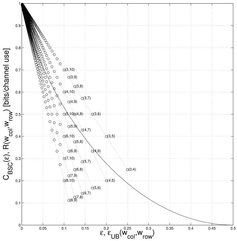
Figure 1: The solid line shows the capacity $C_{\mathrm{BSC}}(\varepsilon)$ of a BSC as a function of the cross-over probability $\varepsilon$. The circles have the following meaning: the circle with label $(w_{\mathrm{col}},w_{\mathrm{row}})$ shows the point $\bigl{(}R(w_{\mathrm{col}},w_{\mathrm{row}}),\varepsilon_{\mathrm{UB}}(w_{\mathrm{col}},w_{\mathrm{row}})\bigr{)}$, where $R(w_{\mathrm{col}},w_{\mathrm{row}})$ and $\varepsilon_{\mathrm{UB}}(w_{\mathrm{col}},w_{\mathrm{row}})$ are the designed rate and the threshold upper bound from Cor. 7, respectively, for $(w_{\mathrm{col}},w_{\mathrm{row}})$-regular LDPC codes.

Example 8

Fig. 1 tries to capture some of the implications of Th. 6 / Cor. 7. The circles in the plot that are to the left of the capacity curve yield non-trivial upper bounds on the error correction capability of LP decoding. (Note that the designed rate of a $(w_{\mathrm{col}},w_{\mathrm{row}})$-regular LDPC code is $1-\frac{w_{\mathrm{col}}}{w_{\mathrm{row}}}$ and that the actual rate is lower bounded by this quantity.) $\square$

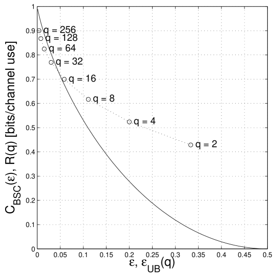
Figure 2: The solid line shows the capacity $C_{\mathrm{BSC}}(\varepsilon)$ of a BSC as a function of the cross-over probability $\varepsilon$. The circles have the following meaning: the circle with label $q$ shows the point $\bigl{(}R(q),\varepsilon_{\mathrm{UB}}(q)\bigr{)}$, where $R(q)$ is the rate of the $\mathrm{PG}(2,q)$-based code and where $\varepsilon_{\mathrm{UB}}(q)$ is the threshold upper bound from Cor. 7 for a family of $(w_{\mathrm{col}}(q),w_{\mathrm{row}}(q))$-regular LDPC codes. (See also the main text for further explanations.)

Example 9

It is a surprising fact that the bounds in Th. 6 and Cor. 7 do not depend on the variable degree $w_{\mathrm{col}}$ at all. In particular, this implies that decoding would fail even if we choose extremely large variable degrees. For example we might consider a sequence of codes defined by parity-check matrices that contain all rows of a given weight $w_{\mathrm{row}}$. Clearly, a specific code $\mathcal{C}_{n}$ of this sequence is a $(\mbox{ \scriptsize$\!\!\left(\!\!\begin{array}[]{c}n-1\\ w_{\mathrm{row}}-1\end{array}\!\!\right)\!$},w_{\mathrm{row}})$-regular code which contains either one ($\mathcal{C}_{n}=\{\mathbf{0}\}$) or two codewords ($\mathcal{C}_{n}=\{\mathbf{0},\mathbf{1}\}$) depending on $k$ being odd or even. Thus, while the rate of this code sequence approaches zero, LP decoding will not succeed for $\varepsilon>\frac{1}{w_{\mathrm{row}}}$. $\square$

Example 10

Th. 6 and Cor. 7 can easily be extended to families of codes where the row weight grows as a function of $n$; let us call theses extensions Th. 6’ and Cor. 7’. It is clear from Cor. 7’ that there cannot be an LP decoding threshold for the BSC if the row weight grows unboundedly. Moreover, coming back to the code family in Ex. 9, if $w_{\mathrm{row}}$ is allowed to grow with $n$, LP decoding will fail as $n\to\infty$ despite the variable degree being exponentially larger than the check degree.

Example 11

Similarly, the family of random codes where entries in a parity-check matrix are drawn independently from a Bernoulli($\theta$) distribution will not only have poor threshold performance under LP decoding but will fail with high probability as the code length approaches infinity for any symmetric channel for which the expression

$$-\frac{\operatorname{E}[\Gamma\,|\,\Gamma{\geq}0]}{\operatorname{E}[\Gamma\,|\,\Gamma{<}0]}\cdot\frac{\operatorname{Pr}(\Gamma{\geq}0)}{\operatorname{Pr}(\Gamma{<}0)}$$

is (upper) bounded. The result follows from the observation that the weight of the rows in $\mathbf{H}$ is exponentially concentrated around $\theta n$. Indeed, given a vector of log-likelihood ratios, the vector with components $\frac{1}{n\theta-\delta-1}$ in positions where $\gamma_{i}$ is non-negative and $1$ in the remaining positions is inside $\mathcal{K}(\mathbf{H})$ with high probability for $\delta>0$ and $n\to\infty$. $\square$

While the above considerations give some insight in the asymptotic behavior of of decoding error for LP decoding, the characterization and spirit of Th. 6 is essentially combinatorial.

Example 12

We saw in Ex. 10 that for any family of codes where the row weight grows as a function of $n$, Cor. 7’ implies that there cannot be an LP decoding threshold for the BSC. A special case, though, arises when the rate of the code family under consideration goes to $1$ when $n\to\infty$ because then also the best code family under the best possible decoding algorithm can only correct a vanishing fraction of bit flips as $n\to\infty$. A family were the rate goes to $1$ as $n\to\infty$ is the family of type-I $\mathrm{PG}(2,q)$-based codes, cf. [13]; in the context of LP decoding, these codes were analyzed in [14, 15]. A code from this family is indexed by $q$ (where $q\triangleq 2^{s}$ for some positive integer $s$), has length $n(q)\triangleq q^{2}+q+1$, rate $R(q)\triangleq 1-(3^{s}+1)/(q^{2}+q+1)$, and $w_{\mathrm{col}}(q)=w_{\mathrm{row}}(q)=q+1$.

Fig. 2 shows the following: for each $q$ we plot the point $(R(q),\varepsilon_{\mathrm{UB}}(q))$, where $R(q)$ is the rate of the $\mathrm{PG}(2,q)$-based code and where $\varepsilon_{\mathrm{UB}}(q)$ is the LP decoding threshold upper bound from Cor. 7 for a $(w_{\mathrm{col}}(q),w_{\mathrm{row}}(q))$-regular family of codes. Care must be taken when giving an interpretation to this figure since the $\mathrm{PG}(2,q)$-based codes are finite-length codes for finite $q$. $\square$

We leave it as an exercise for the reader to generalize the results in this section to irregular LDPC codes.

IV $2$-Neighborhood-Based Bounds on the Threshold for Regular LDPC Codes

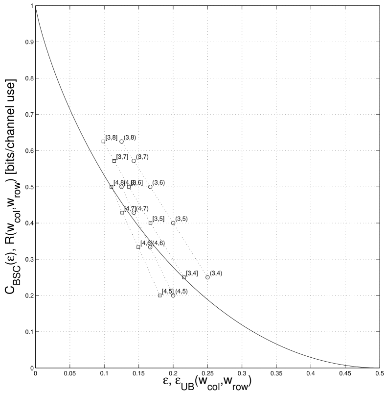
Figure 3: The solid line shows the capacity $C_{\mathrm{BSC}}(\varepsilon)$ of a BSC as a function of the cross-over probability $\varepsilon$. The circles have the same meaning as in Fig. 1. The squares have the following meaning: the square with label $q$ shows the point $\bigl{(}R(q),\varepsilon_{\mathrm{UB}}(q)\bigr{)}$, where $R(q)$ is the rate of the $\mathrm{PG}(2,q)$-based code and where $\varepsilon_{\mathrm{UB}}(q)$ is the $2$-neighborhood-based threshold upper bound from Sec. IV for a family of $(w_{\mathrm{col}}(q),w_{\mathrm{row}}(q))$-regular LDPC codes. (See also the main text for further explanations.)

Because the assignment of a value to $\omega_{i}$ in (5) was only based on the value of $\gamma_{i}$, we call the resulting bound in Cor. 7 a $0$-neighborhood-based bound. (Of course, the way we assigned a value to every $\omega_{i}$ in (5) can also be seen as a very simplistic, and usually sub-optimal way, of solving the linear program in (1).) It is natural to try to formulate more sophisticated assignments of a value to $\omega_{i}$. The next simplest approach is to formulate a rule that does not depend on $\gamma_{i}$ only, but also on $\gamma_{i^{\prime}}$ where $i^{\prime}$ ranges over all variable nodes at Tanner graph distance $2$ from variable node $i$. The resulting bounds on the threshold will therefore be called $2$-neighborhood-based bounds.

For $i\in\mathcal{I}$ let $\mathcal{N}^{(2)}_{i}$ be the subset of $\mathcal{I}$ that includes all variable nodes $i^{\prime}$ with Tanner graph distance at most $2$ from $i$. In the following, we assume that the Tanner graph under consideration has girth at least six. In the case of a $(w_{\mathrm{col}},w_{\mathrm{row}})$-regular LDPC codes, this implies that the set $\mathcal{N}^{(2)}_{i}$ has size $\lvert\mathcal{N}^{(2)}_{i}\rvert=1+w_{\mathrm{col}}(w_{\mathrm{row}}-1)$. (Fig. 4 (left) shows part of a $(3,4)$-regular code, i.e. node $i$, all check nodes at Tanner graph distance $1$ from $i$, and all variable nodes at Tanner graph distance $2$ from $i$.)

Definition 13

Let $\bm{\Gamma}^{\prime}_{i}$ be the vector that contains all the random variables $\{\Gamma_{i^{\prime}}\}_{i^{\prime}\in\mathcal{N}^{(2)}_{i}}$ and let $\bm{\gamma}^{\prime}_{i}$ be its realization. Our new rule (that replaces (5)) for defining a vector $\bm{\omega}\in\mathbb{R}^{n}$ is now $\omega_{i}\triangleq\alpha_{\bm{\gamma}^{\prime}_{i}}$, where $\alpha_{\bm{\gamma}^{\prime}_{i}}\in\mathbb{R}_{+}$ for all $\bm{\gamma}^{\prime}_{i}\in\mathcal{G}^{\lvert\mathcal{N}^{(2)}_{i}\rvert}$ is chosen such that for all possible $\bm{\gamma}\in\mathcal{G}^{n}$ we obtain a vector $\bm{\omega}$ that lies in the fundamental cone.

Lemma 14

Assume that we have such values $\{\alpha_{\bm{\gamma}^{\prime}_{i}}\}_{\bm{\gamma}^{\prime}_{i}}$ as defined in Def. 13. With probability one with have

$$\lim_{n\to\infty}\frac{1}{n}\sum_{i\in\mathcal{I}}\gamma_{i}\omega_{i} =\sum_{\bm{\gamma}^{\prime}_{i}}p_{\bm{\gamma}^{\prime}_{i}}\alpha_{\bm{\gamma}^{\prime}_{i}},$$

where

$$p_{\bm{\gamma}^{\prime}_{i}} \triangleq\Pr\big{(}\{\Gamma_{i^{\prime}}\}_{i^{\prime}\in\mathcal{N}^{(2)}_{i}}=\{\gamma_{i^{\prime}}\}_{i^{\prime}\in\mathcal{N}^{(2)}_{i}}\big{)}=\prod_{i^{\prime}\in\mathcal{N}^{(2)}_{i}}\Pr(\Gamma=\gamma_{i^{\prime}}).$$

Proof: Follows from the fact that $\gamma_{i}\omega_{i}$ depends only on finitely many $\gamma_{i^{\prime}}$ from $\{\gamma_{i^{\prime}}\}_{i^{\prime}\in\mathcal{I}}$ and from the use of the weak law of large numbers. $\square$

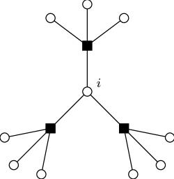
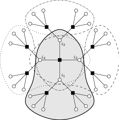
Figure 4: Left: $2$-neighborhood. Right: overlapping $2$-neighborhoods. (See Sec. IV for more explanations.)

Consider a BSC with cross-over probability $\varepsilon$. An upper bound on the LP decoding threshold for the BSC is then given by the infimum of all $\varepsilon$ were we are able to find an assignment in Def. 13 such that $\lim_{n\to\infty}\frac{1}{n}\sum_{i\in\mathcal{I}}\gamma_{i}\omega_{i}$ is negative with probability one. Finding such assignments can e.g. be done by solving a linear program that roughly looks as follows

min. $$\sum_{\bm{\gamma}^{\prime}_{i}}p_{\bm{\gamma}^{\prime}_{i}}\alpha_{\bm{\gamma}^{\prime}_{i}}$$

subj. to $$\alpha_{\tilde{\bm{\gamma}}^{\prime}_{i}}=1$$,

and for each $$\bm{\gamma}$$ the assignment always results in a

$$\text{non-zero vector that lies in the fundamental cone},$$

where $\tilde{\bm{\gamma}}^{\prime}_{i}$ is an arbitrary assignment of values to $\bm{\gamma}^{\prime}_{i}$, e.g. $\gamma_{i^{\prime}}=-G$ for all $i^{\prime}\in\mathcal{N}^{(2)}_{i}$, where $G$ is defined as in Ex. 2.

The Tanner graph in Fig. 4 (left) has many symmetries that can be used to simplify the above linear program. E.g. if there is a graph isomorphism that maps an assignments ${\overline{\bm{\gamma}}}^{\prime}_{i}$ to an assignment ${\overline{\overline{\bm{\gamma}}}}^{\prime}_{i}$, then without loss of generality we can assume that $\alpha_{{\overline{\bm{\gamma}}}^{\prime}_{i}}=\alpha_{{\overline{\overline{\bm{\gamma}}}}^{\prime}_{i}}$. In this way, the dimensionality of the above linear program can be reduced significantly. Without going into the details, the requirement that the resulting assignment always results in a vector in the fundamental cone can be simplified by introducing some auxiliary variables according to overlapping $2$-neighborhoods as is sketched in Fig. 4 (right).

Example 15

Fig. 3 shows the improved upper bounds for $(w_{\mathrm{col}},w_{\mathrm{row}})$-regular code families. $\square$

Whereas the above approach results in relatively small linear programs for small $w_{\mathrm{col}}$ and $w_{\mathrm{row}}$, similar $4$-, $6$-, $8$-, etc., neighborhood-based approaches seem to be computationally much more demanding. We leave it as an open question to see if there are ways to handle also these cases in an efficient numerical way.

References

- [1] N. Wiberg, Codes and Decoding on General Graphs. PhD thesis, Linköping University, Sweden, 1996.
- [2] M. G. Luby, M. Mitzenmacher, M. A. Shokrollahi, D. A. Spielman, and V. Stemann, “Practical loss-resilient codes,” in Proc. 29th Annual ACM Symp. on Theory of Computing, pp. 150–159, 1997.
- [3] M. G. Luby, M. Mitzenmacher, and M. A. Shokrollahi, “Analysis of random processes via and-or tree evaluation,” in Proc. 9th Annual ACM-SIAM Symp. on Discrete Algorithms, pp. 364–373, 1998.
- [4] T. J. Richardson and R. L. Urbanke, “The capacity of low-density parity-check codes under message-passing decoding,” IEEE Trans. on Inform. Theory, vol. IT–47, no. 2, pp. 599–618, 2001.
- [5] M. Lentmaier, D. V. Truhachev, D. J. Costello, Jr., and K. Zigangirov, “On the block error probability of iteratively decoded LDPC codes,” in 5th ITG Conference on Source and Channel Coding, (Erlangen, Germany), Jan. 14-16 2004.
- [6] H. Jin and T. Richardson, “Block error iterative decoding capacity for LDPC codes,” in Proc. IEEE Intern. Symp. on Inform. Theory, (Adelaide, Australia), pp. 52 – 56, Sep. 4–9 2005.
- [7] R. Koetter and P. O. Vontobel, “On the block error probability of LP decoding of LDPC codes,” in Proc. Inaugural Workshop of the Center for Information Theory and its Applications, (UC San Diego, La Jolla, CA, USA), Feb. 6-10 2006.
- [8] S. Boyd and L. Vandenberghe, Convex Optimization. Cambridge, UK: Cambridge University Press, 2004.
-
[9]
J. Feldman, Decoding Error-Correcting Codes via Linear Programming.
PhD thesis, Massachusetts Institute of Technology, Cambridge, MA,
2003.
Available online under
http://www.columbia.edu/~jf2189/pubs.html. - [10] J. Feldman, M. J. Wainwright, and D. R. Karger, “Using linear programming to decode binary linear codes,” IEEE Trans. on Inform. Theory, vol. IT–51, no. 3, pp. 954–972, 2005.
- [11] R. Koetter and P. O. Vontobel, “Graph covers and iterative decoding of finite-length codes,” in Proc. 3rd Intern. Symp. on Turbo Codes and Related Topics, (Brest, France), pp. 75–82, Sept. 1–5 2003.
-
[12]
P. O. Vontobel and R. Koetter, “Graph-cover decoding and finite-length
analysis of message-passing iterative decoding of LDPC codes,” submitted to IEEE Trans. Inform. Theory, available online under
http://www.arxiv.org/abs/cs.IT/0512078, Dec. 2005. - [13] Y. Kou, S. Lin, and M. P. C. Fossorier, “Low-density parity-check codes based on finite geometries: a rediscovery and new results,” IEEE Trans. on Inform. Theory, vol. IT–47, pp. 2711–2736, Nov. 2001.
-
[14]
P. O. Vontobel, R. Smarandache, N. Kiyavash, J. Teutsch, and D. Vukobratovic,
“On the minimal pseudo-codewords of codes from finite geometries,” in Proc. IEEE Intern. Symp. on Inform. Theory, (Adelaide, Australia),
pp. 980–984, Sep. 4–9 2005.
Available online under
http://www.arxiv.org/abs/cs.IT/0508019. -
[15]
P. O. Vontobel and R. Smarandache, “On minimal pseudo-codewords of Tanner
graphs from projective planes,” in Proc. 43rd Allerton Conf. on
Communications, Control, and Computing, (Allerton House, Monticello,
Illinois, USA), Sep. 28–30 2005.
Available online under
http://www.arxiv.org/abs/cs.IT/0510043.