Classifying Signals With Local Classifiers

Abstract

This paper deals with the problem of classifying signals. The new method for building so called local classifiers and local features is presented. The method is a combination of the lifting scheme and the support vector machines. Its main aim is to produce effective and yet comprehensible classifiers that would help in understanding processes hidden behind classified signals. To illustrate the method we present the results obtained on an artificial and a real dataset.

Keywords: local feature, local classifier, lifting scheme, support vector machines, signal analysis

1 Introduction

Many classification algorithms such as artificial neural networks induce classifiers which have good accuracy but do not give an insight into the real process which is hidden behind the problem. Although predictions are made with high precision such classifiers do not answer the question ’’Why?‘‘. Even algorithms such as decision trees or rule inducers very often produce enormous classifiers. Their analysis is almost intractable by the human mind. It is even worse when these algorithms are used for problems of signal classification. In practice good accuracy without an explanation of the classification process is useless.

In this article we describe an approach which can help in building classifiers which are not only very accurate but also comprehensible. The method is based on the idea of the lifting scheme (Sweldens, 1998). The lifting scheme is used for calculating expansion coefficients of analysed signals using biorthogonal wavelet bases. The biggest advantage of this method is that it uses only spatial domain in contrast to the classical approach (Daubechies, 1992) in which the frequency domain is used. As originally lifting scheme did not give us enough freedom in incorporating adaptation we used its modified version called update-first (Claypoole et al., 1998).

Assume we act in space $\mathbb{R}^{N}$ spanned by a biorthogonal base $\{\phi_{i}\}_{i=1}^{n}$ and $\{\tilde{\phi}_{i}\}_{i=1}^{n}$. Vectors $\{\phi_{i}\}_{i=1}^{n}$ and $\{\tilde{\phi}_{i}\}_{i=1}^{n}$ are biorthogonal in the sense that

$$\left\langle\phi_{i},\tilde{\phi_{j}}\right\rangle=\delta_{ij}$$

where $\delta_{ij}=1$ if $i=j$ and $0$ otherwise.

Each vector $x\in\mathbb{R}^{N}$ can be expressed in the following way

$$x=\sum_{i=1}^{n}\alpha_{i}\phi_{i}$$ (1)

where $\alpha_{i}=\left\langle\tilde{\phi}_{i},x\right\rangle$ are expansion coefficients. Very important feature of vectors $\{\tilde{\phi}_{i}\}_{i=1}^{n}$ is that they can be nonzero only for several indices. It implies that for calculating $\left\langle\tilde{\phi}_{i},x\right\rangle$ only a part of the vector $x$ is needed. This feature is called locality.

The aim of the method presented in this article is to find such an expansion (1) by implicitly constructing biorthogonal base $\{(\phi_{i},\tilde{\phi}_{i})\}_{i=1}^{n}$, that coefficients $\alpha_{i}=\left\langle\tilde{\phi}_{i},x\right\rangle$ are as discriminative as possible for classified signals.

More specifically we assume that a training set $X=\{(x_{i},y_{i}):x_{i}\in\mathbb{R}^{n},y_{i}\in\{-1,+1\}\}_{i=1}^{l}$ is given. For each base vector $\tilde{\phi}_{j}$ we get a vector of expansion coefficients $\alpha^{j}\in\mathbb{R}^{l}$

$$\alpha^{j}(i)=\left\langle\tilde{\phi}_{j},x_{i}\right\rangle$$

For each such vector we can find a number $b^{j}\in\mathbb{R}$ called bias for which

$$\mathrm{sgn}(\alpha^{j}(i)+b^{j})=y_{i}$$

for as many indices $i\in\left\{1,2,\ldots,l\right\}$ as possible.

For calculating expansion coefficients we used the idea of support vector machines (SVM) introduced by Vapnik (1998). SVM proved to be one of the best classifier inducers. Combining the power of SVM and the locality feature of the designed base we were able to build classifiers with a very good classification accuracy and which are also easily interpreted. We present experiments obtained for an artificial datasets and a real dataset. The artificial datasets allowed us to verify our method and to better understand its features. Experiments conducted on the real dataset proofed usefulness of the method for real applications.

2 Outline of the paper

The paper is divided into two main parts and the appendix. The first part is devoted to a description of the method and consists of three subparts. First we present a general outline of the method next we introduce some notation that will be used in next part that gives detailed description of the method. The first part of the paper we end with a short summary of the presented method. In the second part of the paper we present a results of the experiments conducted both on the artificial and the real dataset. In the appendix we show how to efficiently solve optimisation problems that arise in the method.

3 Method description

In this section we will describe the new method for designing discriminative biorthogonal bases for signal classification. In fact we will be computing only expansion coefficients of some implicitly defined discriminative biorthogonal base. The method is a combination of update-first version of the lifting scheme (Claypoole et al., 1998) and proximal support vector machines (Fung and Mangasarian, 2001).

3.1 Outline of the method

The method is based on the Lifting Scheme that is very general and easily modified method for computing expansion coefficients of analysed signal with respect to biorthogonal base. The method is iterative and each iteration is divided into three steps

• SPLIT - Signal is splitted into two subsignals containing even and odd indices.

• UPDATE - Coarse approximation of analysed signal is computed from subsignals.

• PREDICT - Wavelet coefficients are calculated using coarse approximation and subsignal containing even indicies. Those coefficients are simply inner products between a weight vector and small part of coarse approximation and even subsignal. We used proximal support vector Machines (Fung and Mangasarian, 2001) to calculate the weight vector. As PSVM is the procedure for generating classifiers we decided to call obtained expansion coefficients discriminative wavelet coefficients.

Coarse approximation is used as an input for next iteration. As the coarse approximation is twice shorter than original signal the number of iterations is bounded from above by $\ln(N)$ where $N$ is the length of the analysed signal.

3.2 Notation

Assume we are given a training set $X$

$$X=\left\{(\mathbf{x}_{i},y_{i})\in\mathbb{R}^{N\times\{-1,+1\}}:i=1,\ldots,l\right\}$$

where $N=2^{n}$ for some $n\in\mathbb{N}$. Vectors $\mathbf{x}_{i}$ are sampled versions of signals we want to analyse and $y_{i}\in\{-1,+1\}$ are labels.

Having set $X$ we create two matrices

$$\mathbf{A}=\left(\begin{array}[]{c}\mathbf{x}_{1}^{T}\\ \vdots\\ \mathbf{x}_{l}^{T}\end{array}\right)\in\mathbb{R}^{l\times N}$$

and

$$\mathbf{Y}=\left(\begin{array}[]{ccc}y_{1}&&\\ &\ddots&\\ &&y_{l}\end{array}\right)$$

Let $I=\{i_{1},\ldots,i_{k}\}$ be a set of integer numbers (indices). We will use the following shorthand notation for accessing indices I of a vector $\mathbf{x}\in\mathbb{R}^{N}$.

$$\mathbf{x}(I)=(\mathbf{x}(i_{1}),\ldots,\mathbf{x}(i_{k}))$$

We will also use a special notation for accessing odd and even indices of a vector $\mathbf{x}\in\mathbb{R}^{N}$

$$\mathbf{x_{o}} = (\mathbf{x}(1),\mathbf{x}(3),\ldots,\mathbf{x}(N-1))\quad\textrm{for odd indices}$$

$$\mathbf{x_{e}} = (\mathbf{x}(2),\mathbf{x}(4),\ldots,\mathbf{x}(N))\quad\textrm{for even indices}$$

Finally we will use the following symbols for special vectors

$$\mathbf{e}=\left(\begin{array}[]{c}1\\ \vdots\\ 1\end{array}\right)$$

and

$$\mathbf{e_{1}}=\left(\begin{array}[]{c}1\\ 0\\ \vdots\\ 0\end{array}\right)$$

The dimensionality of the vectors $\mathbf{e}$ and $\mathbf{e_{1}}$ will be clear from the context.

3.3 Three main steps

As we have mentioned before the method we propose is iterative and each iteration step consists of three substeps.

3.3.1 First substep - Split

Matrix $\mathbf{A}$ is splitted into matrices $\mathbf{A_{o}}$ (odd columns) and $\mathbf{A_{e}}$ (even columns)

$$\mathbf{A_{o}}=\left(\begin{array}[]{c}\mathbf{x_{o}}_{1}^{T}\\ \vdots\\ \mathbf{x_{o}}_{l}^{T}\end{array}\right)\in\mathbb{R}^{l\times N/2}$$

and

$$\mathbf{A_{e}}=\left(\begin{array}[]{c}\mathbf{x_{e}}_{1}^{T}\\ \vdots\\ \mathbf{x_{e}}_{l}^{T}\end{array}\right)\in\mathbb{R}^{l\times N/2}$$

3.3.2 Second substep - Update

Having matrices $\mathbf{A_{o}}\in\mathbb{R}^{l\times N/2}$ and $\mathbf{A_{e}}\in\mathbb{R}^{l\times N/2}$ we create matrix $\mathbf{C}\in\mathbb{R}^{l\times N/2}$

$$\mathbf{C}=\frac{1}{2}\left(\mathbf{A_{o}}+\mathbf{A_{e}}\right)=\left(\begin{array}[]{c}\mathbf{c}_{1}^{T}\\ \vdots\\ \mathbf{c}_{l}^{T}\end{array}\right)$$

This matrix will be called coarse approximation of matrix $\mathbf{A}$.

3.3.3 Third substep - Predict

In the last step we calculate discriminative wavelet coefficients. For each column $k$ of matrix $\mathbf{A_{e}}$ ($k=1,2,\ldots,N/2$) we create matrix $\mathbf{A}^{k}\in\mathbb{R}^{l\times L_{k}+1}$ where $L_{k}\in\mathbb{N}$ is an even number and a parameter of the method.

$$\mathbf{A}^{k}=\left(\begin{array}[]{cc}\mathbf{x_{e}}_{1}(k)&-\mathbf{c}^{k}_{1}\\ \vdots&\vdots\\ \mathbf{x_{e}}_{l}(k)&-\mathbf{c}^{k}_{l}\end{array}\right)$$

where $\mathbf{c}^{k}_{i}=\mathbf{c}_{i}(I_{k})$ and $I_{k}$ is a set of indices selected in the following way

• If $1\leq k<\frac{L_{k}}{2}$ then $I_{k}=\{1,2,\ldots,L_{k}\}$

• If $\frac{L_{k}}{2}\leq k<\frac{N}{2}-\frac{L_{k}}{2}$ then $I_{k}=\{k-\frac{L_{k}}{2}+1,\ldots,k+\frac{L_{k}}{2}\}$

• If $\frac{N}{2}-\frac{L_{k}}{2}\leq k\leq\frac{N}{2}$ then $I_{k}=\{\frac{N}{2}-L_{k}+1,\ldots,\frac{N}{2}\}$

At this point our method can be splitted into two variants: regularised and non-regularised.

• regularised variant: This variant uses PSVM approach to find the optimal weight vector $\mathbf{w}^{k}\in\mathbb{R}^{L_{k}+1}$. According to Fung and Mangasarian (2001) optimal $\mathbf{w}^{k}$ is the solution of the following optimisation problem

  $$min_{\mathbf{w}^{k},\gamma_{k},\mathbf{\xi}^{k}}\frac{1}{2}\|\mathbf{w}^{k}\|^{2}_{2}+\frac{1}{2}\gamma_{k}^{2}+\frac{\nu_{k}}{2}\|\mathbf{\xi}_{k}\|^{2}_{2}$$ (2)

  subject to constraints

  $$\mathbf{Y}(\mathbf{A}^{k}\mathbf{w}^{k}-\gamma_{k}\mathbf{e})+\mathbf{\xi}^{k}=\mathbf{e}$$ (3)

  where $\xi^{k}$ is the error vector and $\nu^{k}\geq 0$.

• non-regularised variant: Similarly as in regularised variant the optimal weight vector $\mathbf{w}^{k}\in\mathbb{R}^{L_{k}}$ is given by solving the following optimisation problem

  $$min_{\mathbf{w}^{k},\gamma_{k},\mathbf{\xi}^{k}}\frac{1}{2}\|\mathbf{w}^{k}\|^{2}_{2}+\frac{1}{2}\gamma_{k}^{2}+\frac{\nu_{k}}{2}\|\mathbf{\xi}_{k}\|^{2}_{2}$$ (4)

  subject to constraints

  $$\mathbf{Y}\left(\mathbf{A}^{k}\left(1\atop\mathbf{w}^{k}\right)-\gamma_{k}\mathbf{e}\right)+\mathbf{\xi}^{k}=\mathbf{e}$$ (5)

  where $\xi^{k}$ is the error vector and $\nu^{k}\geq 0$. The only difference to the previous variant is that dimensionality of $\mathbf{w}^{k}$ is $L_{k}$ instead of $L_{k}+1$ and $x_{ei}(k)$ is multiplied by one.

  In this variant we can also add some extra constraints such that in case of polynomial signals (up to some degree $p_{k}$) we will get wavelet coefficients equal to zero. These constraints can be written in the following way

  $$\mathbf{B}^{k}\mathbf{w}^{k}=\mathbf{e_{1}}$$ (6)

  where $\mathbf{e_{1}}\in\mathbb{R}^{p_{k}}$ and $\mathbf{B}^{k}$ consists of the first $p_{k}$ rows of the Vandermonde matrix for some knots $t_{1},t_{2},\ldots,t_{L_{k}}$. For more details on how to select knots we refer reader to (Claypoole et al., 1998) and (Fernández et al., 1996).

  The additional constraints could be useful if analysed signals are superposition of polynomial and some other possibly interesting component. They imply that polynomial part of the analysed signal is eliminated and thus interesting component will play a bigger role in constructing discriminative wavelets coefficients. Also constructed base will have similar properties to the standard wavelet base. In the appendix the reader can find information on how to efficiently solve this extended optimisation problem. We have not used this variant in our experiments but present it for completeness reasons.

Having optimal weight vector $\mathbf{w}^{k}$ we can calculate vector $\mathbf{d}^{k}\in\mathbb{R}^{l}$ of discriminative wavelet coefficients using the following equations

• regularised variant

  $$\mathbf{d}^{k}(i)=\left\langle\mathbf{w}^{k},\left(\mathbf{x_{e}}_{i}(k)\atop-\mathbf{c}^{k}_{i}\right)\right\rangle\quad i=1,2,\ldots,l$$

• non-regularised variant

  $$\mathbf{d}^{k}(i)=\mathbf{x_{e}}_{i}(k)-\left\langle\mathbf{w}^{k},\mathbf{c}^{k}_{i}\right\rangle\quad i=1,2,\ldots,l$$

  where $\left\langle\cdot,\cdot\right\rangle$ is a standard inner product.

In a result we obtain a matrix $\mathbf{D}\in\mathbb{R}^{l\times N/2}$

$$\mathbf{D}=\left(\begin{array}[]{ccc}\mathbf{d}^{1}&\cdots&\mathbf{d}^{N/2}\end{array}\right)$$

3.4 Iteration step

The whole algorithm can be written in the following form

• Let $M$ be the number of iterations (decomposition levels).

• Let $\mathbf{A}_{0}$=$\mathbf{A}$

• For $m=1,\ldots,M$ do

  • Calculate $\mathbf{C}_{m}\in\mathbb{R}^{l\times\frac{N}{2^{m}}}$ and $\mathbf{D}_{m}\in\mathbb{R}^{l\times\frac{N}{2^{m}}}$ by applying three steps described in the previous section to the matrix $\mathbf{A}_{m-1}$.

  • Set $\mathbf{A}_{m}=\mathbf{C}_{m}$.

The output of the algorithm will be a set of matrices $\mathbf{C}_{M},\mathbf{D}_{1},\ldots,\mathbf{D}_{M}$. On the basis of these matrices we create the new training set

$$X^{new}=\left\{(\mathbf{x}^{new}_{i},y_{i})\in\mathbb{R}^{N\times\{-1,+1\}}:i=1,\ldots,l\right\}$$ (7)

where new examples are created by merging rows of matrices $\mathbf{C}_{M},\mathbf{D}_{1},\ldots,\mathbf{D}_{M}$.

3.5 Method summary

We introduced the method that maps the set of signals $X$ into a new set of signals $X^{new}$. In the presented setting this map is a linear and invertible function $f\colon\mathbb{R}^{N}\to\mathbb{R}^{N}$

$$f(x)=(\mathbf{c}_{M}^{T},\mathbf{d}_{1}^{T},\ldots,\mathbf{d}_{M}^{T})$$

where

$$\mathbf{c}_{M} \in \mathbb{R}^{\frac{N}{2^{M}}}$$

$$\mathbf{d}_{M} \in \mathbb{R}^{\frac{N}{2^{M}}}$$

$$\vdots$$

$$\mathbf{d}_{2} \in \mathbb{R}^{\frac{N}{4}}$$

$$\mathbf{d}_{1} \in \mathbb{R}^{\frac{N}{2}}$$

are calculated by the method. With increasing $m$ more and more samples from the original signal is used to calculate expansion coefficients. For example if we set $L_{k}\equiv L$ for all $k$ then to calculate vector $\mathbf{d}^{k}$ $L2^{m}$ samples of the original signal will be used.

Here we present two most important features of the method

• Motivation for the method is that only a small part of the signals is important in classification process. The method tries to identify this important part adaptively.

• Exploiting natural parallelism (calculating $\mathbf{d}^{k}$ is completely independent for each $k$) and Sherman-Morrison-Woodbury formula (Gene H. Golub, 1996) the method can be implemented very efficiently. In the appendix A we show how to properly solve optimisation problems that appears in our method.

4 Applications

This section contains description of possible applications of the proposed method. It is divided into two parts. In the first part we present an illustrative example of analysing artificial signals with the proposed method. In the second part we present the results for the real dataset.

4.1 Artificial datasets

Here we present results obtained on artificial datasets: Waveform and Shape.

4.1.1 Dataset description

Waveform is a three class artificial dataset (Breiman, 1998). For our experiments we used a slightly modified version (Saito, 1994). Three classes of signals were generated using the following formulas

$$x^{1}(i) = uh_{1}(i)+(1-u)h_{2}(i)+\epsilon(i)\quad\textrm{class 1}$$ (8)

$$x^{2}(i) = uh_{1}(i)+(1-u)h_{3}(i)+\epsilon(i)\quad\textrm{class 2}$$ (9)

$$x^{3}(i) = uh_{2}(i)+(1-u)h_{3}(i)+\epsilon(i)\quad\textrm{class 3}$$ (10)

where $i=1,2,\ldots,32$, $u$ is a uniform random variable on the interval $(0,1)$, $\epsilon(i)$ is a standard normal variable and

$$h_{1}(i) = max(6-|i-7|,0)$$

$$h_{2}(i) = h_{1}(i-8)$$

$$h_{3}(i) = h_{1}(i-4)$$

4.1.2 Analysis

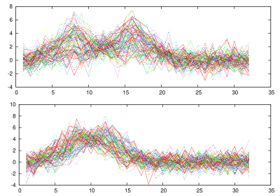
Figure 1: Examples from classes 1 and 2

For simplicity reasons we decided to concentrate only on classes 1 and 2 presented in the Figure 1. For the purpose of this presentation we set parameters of our method as follows

$$L_{k} = 4$$

$$\nu_{k} = 1$$

$$M = 3$$

Figure 2 presents coarse approximations (the first two rows) and the test error ratio (the third row) of calculated discriminative wavelet coefficients (evaluated on a separate test set). Each column present distinct decomposition level of our method. It is easily seen that coarse approximations are an averaged and a shortened versions of original signals. We believe that in some cases such averaging could be very useful especially when the analysed signals contains much noise. From the last row of the Figure 2 we can deduce that the classification ratio of some discriminative wavelet coefficients is comparable to the classification ratio obtained by applying PSVM method to the original dataset. We can point out explicitly the period of time in which two classes of signals differ most. This feature we called locality. Let us take a closer look at the $6$th discriminative wavelet coefficient from the first decomposition level. To calculate this coefficient we need $8$ out of $32$ samples of analysed signals (see first row of the Figure 3).

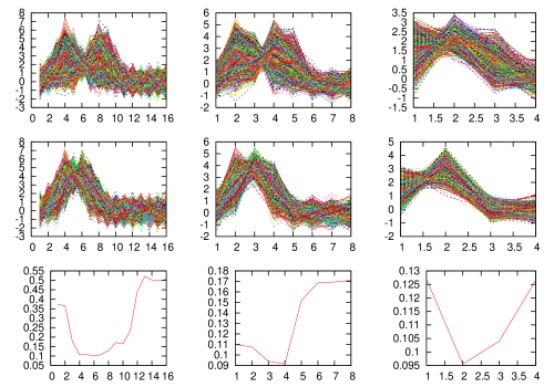
Figure 2: Coarse approximations (two upper rows) and test error of discriminative wavelet coefficients (third row) for examples from classes 1 and 2.

In the Figure 3 one can see that base analysis vectors with the lowest error ratio have the supports shorter than their length. This means that to discern classes 1 and 2 we do not need all 32 samples but only a small fraction of them. Moreover when comparing Figures 1 and 3 it is clear that best analysis base vectors are nonzero where supports of functions $h_{1}$ and $h_{3}$ intersect and this is the place where analysed signals indeed differ.

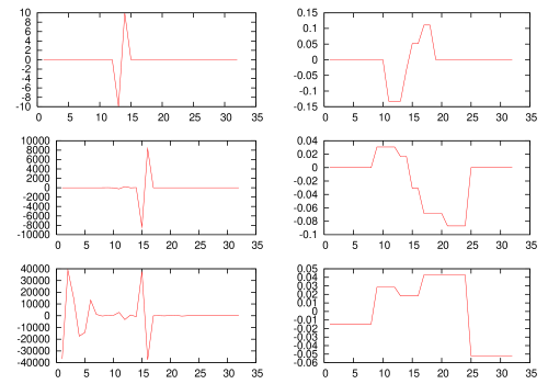
Figure 3: Best synthesis (left) and analysis (right) base vectors for each decomposition level

The last Figure 4 shows supports of analysis and synthesis base vectors. It is easily seen that support of a base vector widens with decomposition level.

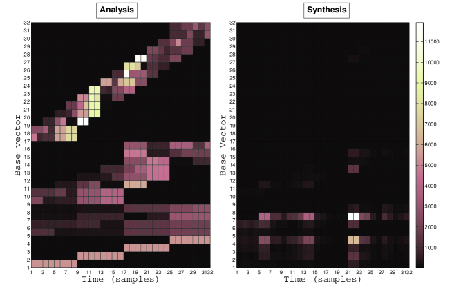
Figure 4: Supports of analysis and synthesis discriminative base

4.1.3 Extracting new features

The method we presented can also be used as a supervised feature extractor. Instead of feeding classifier with original training set $X$ we use $X^{new}$ defined in (7). Table 1 contains results of replacing original data with new features for classifying Waveform dataset and Shape dataset (Saito, 1994) with C4.5 classifier (Ian H. Witten, 1999). From this table we can derive that classification ratio increased considerably. We have also noticed a substantial decrease of decision tree complexity. As our method is designed for two-class problems and the used datasets are three-class problems we used one-against-one scheme (jen Lin and wei Hsu, 2001).

Dataset	Misclassification ratio
	Original	New
Waveform	$0.290$	$0.186$
Shape	$0.081$	$0.023$

Table 1: Effect of feature extraction for C4.5. Numbers are misclassification ratios.

4.1.4 Ensemble of local classifiers

The coefficients calculated by our method can also be used directly for classification. Table 2 contains the test error ratios for Waveform and Shape datasets obtained by voting few best coefficients. As in the previous experiment we used one-against-one scheme for decomposing multi-class problems into three two-class problems.

Dataset	Misclassification ratio
	$3$ coefficients	$15$ coefficients	PSVM
Waveform	$0.155$	$0.147$	$0.193$
Shape	$0.034$	$0.032$	$0.094$

Table 2: Misclassification ratios for voting scheme. We were combining 3 and 15 coefficients. The last column shows the misclassification ratio obtained using PSVM and all samples.

4.1.5 Conclusions

The presented method give both accurate and comprehensible solution to classification problems. It can be very useful not only as a classifier inducer but also as source of information about classified signals. In the next section we support our claims with presenting the results obtained on the real dataset.

4.2 Classifying evoked potentials

In this section we present the results obtained on the dataset collected in Nencki Institute of Experimental Biology of Polish Academy of Science. The dataset consists of sampled evoked potentials of rat‘s brain recorded in two different conditions. As a result the dataset consists of two groups of recordings (CONTROL and COND) that represent two different states of the rat‘s brain. The aim of the experiment was to explain the differences between the two groups. We refer the reader to Kublik et al. (2001) and Wypych et al. (2003) for more details and previous approaches to the data.

It should be mentioned that the problem is not a typical classification task. This is due to the following reasons

• Each example (evoked potential) is labelled with an unknown noise. It means that there are examples that are possibly incorrectly labelled.

• The problem is ill-conditioned due to a small number of examples (45-100) and a huge dimension (1500 samples).

• The biologists that collected the data were interested not only in a good classification ratio but also in explanation of differences in the two groups.

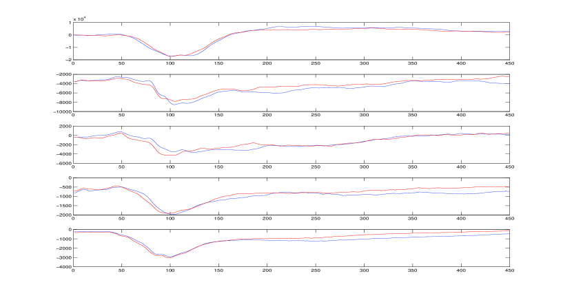
Figure 5: Averaged evoked potentials for five rats. Red colour denotes COND and blue denotes CONTROL. Only first most informative 45ms (450 samples) are presented.

Figure 5 presents averaged potentials from two classes for group of five rats. We show only the first 45ms because differences in this period of time can be easily interpreted by biologists.

After applying our method to evoked potentials for each rat we have chosen those local classifiers whose classification accuracy was greater or equal $0.75$ and it was statistically significant at the level $0.1$ with respect to permutation tests (Wypych et al., 2003). The result of this selection is depicted in the Figure 6. It is clear that the most interesting parts of the signals are $2.9$-$4$ms and $11.7$-$12.8$ms. Figure 7 shows how each potential is classified by selected local classifiers. It should be read in the following manner

• Vertical line divides potentials into two groups CONTROL (on the left) and COND (on the right).

• Axis Y shows how selected classifiers agreed on classifying potential.

• The potentials were grouped (red and blue) depending on how they were classified. Those marked with green colour could not be classified.

• We claim that those groups shows two different states of the rat‘s brain.

The presented method gave very similar results to the previous approaches (Kublik et al., 2001), (Wypych et al., 2003) and (Smolinski et al., 2002). Thanks to locality feature of our method we were able not only to classify potentials but also to point out the most informative part of the signals. For detailed physiological interpretation of the results we refer the reader to Jakuczun et al. (2005).

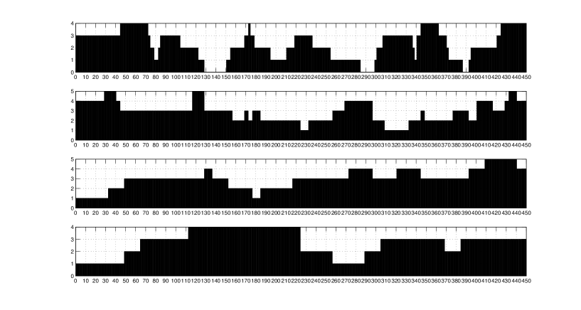
Figure 6: Histograms showing which parts of analysed signals are commonly indicated for all rats. The picture shows first four levels of decomposition of our method.

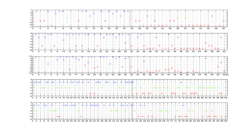
Figure 7: Charts presenting how particular potential was classified by selected local classifiers. Vertical line divides potentials into two groups (CONTROL is on the left, COND is on the right).

5 Conclusions

In this article we presented a new method for classifying signals. The method is iterative and adapts to local structures of analysed signals. If carefully implemented it can be very efficient and when used by an experienced researcher can be a very powerful tool for signals discriminative analysis. There are many possible extensions to our method but the most interesting seem to be the following

• Modification of the method to handle two dimensional signals such us images.

• Applying kernel trick in constructing local classifiers. That would lead to nonlinear classifiers and possibly better accuracy.

• Constructing classifiers using Multi Kernel Learning approaches (Bach et al., 2004).

A Efficiently solving optimisation problem for non-regularised and regularised version

Here we explain how to efficiently solve optimisation problem defined by (4), (5), (6). Let us write Lagrangian for the optimisation problem

$$L(\mathbf{w}^{k},\gamma_{k},\mathbf{\xi}^{k},\mathbf{u}^{k},\mathbf{v}^{k}) = \frac{1}{2}(\|\mathbf{w}^{k}\|^{2}_{2}+\gamma_{k}^{2})+\frac{\nu_{k}}{2}\|\mathbf{\xi}^{k}\|^{2}_{2}+$$

$$- (\mathbf{u}^{k})^{T}\left(\mathbf{Y}\left(\mathbf{A}^{k}\left(1\atop\mathbf{w}^{k}\right)-\gamma_{k}\mathbf{e}\right)+\mathbf{\xi}^{k}-\mathbf{e}\right)$$

$$- (\mathbf{v}^{k})^{T}\left(\mathbf{B}^{k}\mathbf{w}^{k}-\mathbf{e_{1}}\right)$$

where $\mathbf{u}^{k}\in\mathbb{R}^{l}$ is the Lagrange multiplier associate with the equality constraint (5) and $\mathbf{v}^{k}\in\mathbb{R}^{p_{k}}$ is the Lagrange multiplier associated with the equality constraint (6).

Settings the gradients of L to zero we get the following optimality conditions

$$\mathbf{w}^{k} = (\mathbf{\tilde{\tilde{A}}}^{k})^{T}\mathbf{Y}\mathbf{u}^{k}-(\mathbf{B}^{k})^{T}\mathbf{v}^{k}$$ (12)

$$\gamma_{k} = -\mathbf{e}^{T}\mathbf{Y}\mathbf{u}^{k}$$ (13)

$$\mathbf{\xi}^{k} = \frac{1}{\nu^{k}}\mathbf{u}^{k}$$ (14)

$$\mathbf{Y}\left(\mathbf{\tilde{A}}^{k}+\mathbf{\tilde{\tilde{A}}}^{k}\mathbf{w}^{k}-\gamma_{k}\mathbf{e}\right)+\mathbf{\xi}^{k} = \mathbf{e}$$ (15)

$$\mathbf{B}^{k}\mathbf{w}^{k} = \mathbf{e_{1}}$$ (16)

where $\mathbf{A}^{k}=\left(\mathbf{\tilde{A}}^{k}\mathbf{\tilde{\tilde{A}}}^{k}\right)$

Substituting (12) into (16) we get

$$\mathbf{v}^{k}=\left[\mathbf{B}^{k}\left(\mathbf{B}^{k}\right)^{T}\right]^{-1}\left(\mathbf{B}^{k}\left(\mathbf{\tilde{\tilde{A}}}^{k}\right)^{T}\mathbf{Y}\mathbf{u}^{k}-\mathbf{e}\right)$$ (17)

Substituting (12), (13), (14) and (17) into (15) we get

$$\mathbf{Y}\left\{\mathbf{\tilde{\tilde{A}}}^{k}\left(\mathbf{\tilde{\tilde{A}}}^{k}\right)^{T}\mathbf{Y}\mathbf{u}^{k}-\mathbf{\tilde{\tilde{A}}}^{k}\left(\mathbf{B}^{k}\right)^{T}\left[\mathbf{B}^{k}\left(\mathbf{B}^{k}\right)^{T}\right]^{-1}\left(\mathbf{B}^{k}\left(\mathbf{\tilde{\tilde{A}}}^{k}\right)^{T}\mathbf{Y}\mathbf{u}^{k}-\mathbf{e}\right)\right\}+\frac{1}{\nu^{k}}\mathbf{u}^{k}=\mathbf{e}-\mathbf{Y}\mathbf{\tilde{A}}^{k}$$ (18)

Simplifying (18) we get

$$\begin{array}[]{rcl}\mathbf{Y}\left\{\mathbf{\tilde{\tilde{A}}}^{k}\left(\mathbf{\tilde{\tilde{A}}}^{k}\right)^{T}-\mathbf{\tilde{\tilde{A}}}^{k}\left(\mathbf{B}^{k}\right)^{T}\left[\mathbf{B}^{k}\left(\mathbf{B}^{k}\right)^{T}\right]^{-1}\mathbf{B}^{k}\left(\mathbf{\tilde{\tilde{A}}}^{k}\right)^{T}\right\}\mathbf{Y}\mathbf{u}^{k}+\frac{1}{\nu^{k}}\mathbf{u}^{k}&=&\\ =\mathbf{e}-\mathbf{Y}\mathbf{\tilde{A}}^{k}-\mathbf{\tilde{\tilde{A}}}^{k}\left(\mathbf{B}^{k}\right)^{T}\left[\mathbf{B}^{k}\left(\mathbf{B}^{k}\right)^{T}\right]^{-1}\mathbf{e}&&\end{array}$$ (19)

Let matrix $\mathbf{H}_{1}^{k}$ be defined as

$$\mathbf{H}_{1}^{k}=\mathbf{Y}\left[\mathbf{\tilde{\tilde{A}}}^{k}|-\mathbf{\tilde{\tilde{A}}}^{k}\left(\mathbf{B}^{k}\right)^{T}\left(\mathbf{C}^{k}\right)^{T}\right]$$ (20)

and matrix $\mathbf{H}_{2}^{k}$ be defined as

$$\mathbf{H}_{2}^{k}=\mathbf{Y}\left[\mathbf{\tilde{\tilde{A}}}^{k}|\mathbf{\tilde{\tilde{A}}}^{k}\left(\mathbf{B}^{k}\right)^{T}\left(\mathbf{C}^{k}\right)^{T}\right]$$ (21)

where

$$\left[\mathbf{B}^{k}\left(\mathbf{B}^{k}\right)^{T}\right]^{-1}=\left(\mathbf{C}^{k}\right)^{T}\mathbf{C}^{k}$$

Rewriting equation (19) we obtain that

$$\left(\frac{1}{\nu_{k}}\mathbf{I}+\mathbf{H}_{1}\left(\mathbf{H}_{2}\right)^{T}\right)\mathbf{u}^{k}=\mathbf{e}-\mathbf{Y}\mathbf{\tilde{A}}^{k}-\mathbf{\tilde{\tilde{A}}}^{k}\left(\mathbf{B}^{k}\right)^{T}\left[\mathbf{B}^{k}\left(\mathbf{B}^{k}\right)^{T}\right]^{-1}\mathbf{e}$$ (22)

Setting vector $\mathbf{b}^{k}=\mathbf{e}-\mathbf{Y}\mathbf{\tilde{A}}^{k}-\mathbf{\tilde{\tilde{A}}}^{k}\left(\mathbf{B}^{k}\right)^{T}\left[\mathbf{B}^{k}\left(\mathbf{B}^{k}\right)^{T}\right]^{-1}\mathbf{e}$ we get that vector $\mathbf{u}^{k}$ is given by the following set of equations

$$\left(\frac{1}{\nu_{k}}\mathbf{I}+\mathbf{H}_{1}\left(\mathbf{H}_{2}\right)^{T}\right)\mathbf{u}^{k}=\mathbf{b}^{k}$$ (23)

Solving above set of equations is very expensive as the number of equations is equal to number of training examples $l$ which can be large. Using the Sherman-Morrison-Woodbury formula (Gene H. Golub, 1996) we can calculate $\mathbf{u}^{k}$ as follows

$$\mathbf{u}^{k}=\nu_{k}\left(\mathbf{I}-\mathbf{H}_{1}\left(\frac{1}{\nu_{k}}\mathbf{I}+\left(\mathbf{H}_{1}\right)^{T}\mathbf{H}_{2}\right)^{-1}\left(\mathbf{H}_{2}\right)^{T}\right)\mathbf{b}^{k}$$ (24)

It should be stressed that using equation (24) for computing $\mathbf{u}_{k}$ is much less expensive than using equation (23) because the dimensions of matrix

$$\frac{1}{\nu_{k}}\mathbf{I}+\left(\mathbf{H}_{1}\right)^{T}\mathbf{H}_{2}$$

are equal to $L_{k}+p_{k}\times L_{k}+p_{k}$ which is independent of the number of training of examples.

Similarly to nonregularised variant presented above we can use the same techniques to solve optimisation problem (2) and (3). For more details see (Fung and Mangasarian, 2001).

References

- Bach et al. (2004) Francis R. Bach, Gert R. G. Lanckriet, and Michael I. Jordan. Multiple kernel learning, conic duality, and the smo algorithm. In ICML ‘04: Proceedings of the twenty-first international conference on Machine learning, New York, NY, USA, 2004. ACM Press. ISBN 1-58113-828-5. doi: http://doi.acm.org/10.1145/1015330.1015424.
- Breiman (1998) L. Breiman. Arcing classifiers. 1998. URL http://citeseer.ist.psu.edu/breiman98arcing.html.
- Claypoole et al. (1998) R. Claypoole, R. Baraniuk, and R. Nowak. Adaptive wavelet transforms via lifting. 1998. URL http://citeseer.ist.psu.edu/claypoole98adaptive.html.
- Daubechies (1992) Ingrid Daubechies. Ten Lectures on Wavelets. SIAM, 1992.
- Fernández et al. (1996) G. Fernández, S. Periaswamy, and Wim Sweldens. LIFTPACK: A software package for wavelet transforms using lifting. In M. Unser, A. Aldroubi, and A. F. Laine, editors, Wavelet Applications in Signal and Image Processing IV, pages 396–408. Proc. SPIE 2825, 1996.
- Fung and Mangasarian (2001) Glenn Fung and O. L. Mangasarian. Proximal support vector machine classifiers. In Knowledge Discovery and Data Mining, pages 77–86, 2001. URL citeseer.ist.psu.edu/515368.html.
- Gene H. Golub (1996) Charles F. Van Loan Gene H. Golub. Matrix Computations. The Johns Hopkins University Press, 1996.
- Ian H. Witten (1999) Eibe Frank Ian H. Witten. Data Mining: Practical Machine Learning Tools and Techniques with Java Implementations. Morgan Kaufmann, 1999.
- Jakuczun et al. (2005) W. Jakuczun, A. Wróbel, D. Wójcik, and E. Kublik. Classifying evoked potentials with local classifiers. (in preparation), 2005.
- jen Lin and wei Hsu (2001) Chih jen Lin and Chih wei Hsu. A comparison of methods for multi-class support vector machines, June 07 2001. URL http://citeseer.ist.psu.edu/537288.html;http://www.csie.ntu.edu.tw/~cjlin/papers/multisvm.ps.gz.
- Kublik et al. (2001) E. Kublik, P. Musiał, and A. Wróbel. Identification of principal components in cortical evoked potentials by brief suface cooling. Clinical Neuropshysiology, 2001.
- Saito (1994) Naoki Saito. Local Feature Extraction and Its Application Using a Library of Bases. PhD thesis, Yale University, 1994. URL http://www.math.ucdavis.edu/~saito/publications/saito˙phd.html.
- Smolinski et al. (2002) Tomasz G. Smolinski, Grzegorz M. Boratyn, Mariofanna Milanova, Jacek M. Zurada, and Andrzej Wrobel. Evolutionary algorithms and rough sets-based hybrid approach to classificatory decomposition of cortical evoked potentials. In James J. Alpigini, James F. Peters, Andrzej Skowron, and Ning Zhong, editors, Rough Sets and Current Trends in Computing, Third International Conference, RSCTC 2002, number 2475 in Lecture Notes in Artificial Intelligence, pages 621–628. Springer-Verlag, 2002. URL citeseer.csail.mit.edu/smolinski02evolutionary.html.
- Sweldens (1998) Wim Sweldens. The lifting scheme: A construction of second generation wavelets. SIAM Journal on Mathematical Analysis, 29(2):511–546, 1998. URL http://citeseer.ist.psu.edu/sweldens98lifting.html.
- Vapnik (1998) Vladimir Vapnik. Statistical Learning Theory. John Wiley & Sons, 1998.
- Wypych et al. (2003) M. Wypych, E. Kublik, P. Wojdyłło, and A. Wróbel. Sorting functional classes of evoked potentials by wavelets. Neuroinformatic, 2003.