Single-Symbol Maximum Likelihood Decodable Linear STBCs

Abstract

Space-Time block codes (STBC) from Orthogonal Designs (OD) and Co-ordinate Interleaved Orthogonal Designs (CIOD) have been attracting wider attention due to their amenability for fast (single-symbol) ML decoding, and full-rate with full-rank over quasi-static fading channels. However, these codes are instances of single-symbol decodable codes and it is natural to ask, if there exist codes other than STBCs form ODs and CIODs that allow single-symbol decoding?

In this paper, the above question is answered in the affirmative by characterizing all linear STBCs, that allow single-symbol ML decoding (not necessarily full-diversity) over quasi-static fading channels-calling them single-symbol decodable designs (SDD). The class SDD includes ODs and CIODs as proper subclasses. Further, among the SDD, a class of those that offer full-diversity, called Full-rank SDD (FSDD) are characterized and classified.

We then concentrate on square designs and derive the maximal rate for square FSDDs using a constructional proof. It follows that (i) except for $N=2$, square Complex ODs are not maximal rate and (ii) square FSDD exist only for 2 and 4 transmit antennas. For non-square designs, generalized co-ordinate-interleaved orthogonal designs (a superset of CIODs) are presented and analyzed.

Finally, for rapid-fading channels an equivalent matrix channel representation is developed, which allows the results of quasi-static fading channels to be applied to rapid-fading channels. Using this representation we show that for rapid-fading channels the rate of single-symbol decodable STBCs are independent of the number of transmit antennas and inversely proportional to the block-length of the code. Significantly, the CIOD for two transmit antennas is the only STBC that is single-symbol decodable over both quasi-static and rapid-fading channels.

I Introduction

Since the publication of capacity gains of MIMO systems [1, 2] coding for MIMO systems has been an active area of research and such codes have been christened Space-Time Codes (STC). The primary difference between coded modulation (used for SISO, SIMO) and space-time codes is that in coded modulation the coding is in time only while in space-time codes the coding is in both space and time and hence the name. Space-time Codes (STC) can be thought of as a signal design problem at the transmitter to realize the capacity benefits of MIMO systems [1, 2], though, several developments towards STC were presented in [3, 4, 5, 6, 7] which combine transmit and receive diversity, much prior to the results on capacity. Formally, a thorough treatment of STCs was first presented in [8] in the form of trellis codes (Space-Time Trellis Codes (STTC)) along with appropriate design and performance criteria,

The decoding complexity of STTC is exponential in bandwidth efficiency and required diversity order. Starting from Alamouti [12], several authors have studied Space-Time Block Codes (STBCs) obtained from Orthogonal Designs (ODs) and their variations that offer fast decoding (single-symbol decoding or double-symbol decoding) over quasi-static fading channels [9]-[20], [21]-[27]. But the STBCs from ODs are a class of codes that are amenable to single-symbol decoding. Due to the importance of single-symbol decodable codes, need was felt for rigorous characterization of single-symbol decodable linear STBCs.

Following the spirit of [11], by a linear STBC we mean those covered by the following definition.

Definition 1 ( Linear STBC)

A linear design, $S$, is a $L\times N$ matrix whose entries are complex linear combinations of $K$ complex indeterminates $x_{k}=x_{kI}+{\mathbf{j}}x_{kQ}$, $k=0,\cdots,K-1$ and their complex conjugates. The STBC obtained by letting each indeterminate to take all possible values from a complex constellation ${\mathcal{A}}$ is called a linear STBC over ${\mathcal{A}}$. Notice that $S$ is basically a “design”and by the STBC $(S,{\mathcal{A}})$ we mean the STBC obtained using the design $S$ with the indeterminates taking values from the signal constellation ${\mathcal{A}}$. The rate of the code/design is given by $K/L$ symbols/channel use. Every linear design $S$ can be expressed as

$$S=\sum_{k=0}^{K-1}x_{kI}A_{2k}+x_{kQ}A_{2k+1}$$ (1)

where $\{A_{k}\}_{k=0}^{2K-1}$ is a set of complex matrices called weight matrices of $S$. When the signal set ${\mathcal{A}}$ is understood from the context or with the understanding that an appropriate signal set ${\mathcal{A}}$ will be specified subsequently, we will use the terms Design and STBC interchangeably.

Throughout the paper, we consider only those linear STBCs that are obtained from designs. Linear STBCs can be decoded using simple linear processing at the receiver with algorithms like sphere-decoding [38, 39] which have polynomial complexity in, $N$, the number of transmit antennas. But STBCs from ODs stand out because of their amenability to very simple (linear complexity in $N$) decoding. This is because the ML metric can be written as a sum of several square terms, each depending on at-most one variable for OD. However, the rates of ODs is restrictive; resulting in search of other codes that allow simple decoding similar to ODs. We call such codes “single-symbol decodable”. Formally

Definition 2 (Single-symbol Decodable (SD) STBC)

A Single-symbol Decodable (SD) STBC of rate $K/L$ in $K$ complex indeterminates $x_{k}=x_{kI}+{\mathbf{j}}x_{kQ}$, $k=0,\cdots,K-1$ is a linear STBC such that the ML decoding metric can be written as a square of several terms each depending on at most one indeterminate.

Examples of SD STBCs are STBCs from Orthogonal Designs of [9].

In this paper, we first characterize all linear STBCs that admit single-symbol ML decoding, (not necessarily full-rank) over quasi-static fading channels, the class of Single-symbol Decodable Designs (SDD). Further, we characterize a class of full-rank SDDs called Full-Rank SDD (FSDD).

Fig. 1 shows the various classes of SD STBCs identified in this paper. Observe that the class of FSDD consists of only

• an extension of Generalized Linear Complex Orthogonal Design (GLCOD) which we have called Unrestricted Full-rank Single-symbol Decodable Designs (UFSDD) and

• a class of non-UFSDDs called Restricted Full-rank Single-symbol Decodable Designs (RFSDD).

The rest of the material of this paper is organized as follows: In section II the channel model and the design criteria for both quasi-static and rapid-fading channels are reviewed. A brief presentation of basic, well known results concerning GLCODs is given in Section III. In Section IV we characterize the class SDD of all SD (not necessarily full-rank) designs and within the class of SDD the class FSDD consisting of full-diversity SDD is characterized. Section V deals exclusively with the maximal rate of square designs and construction of such maximal rate designs.

In Section VI we generalize the construction of square RFSDDs given in Subsection IV-B, and give a formal definition for Co-ordinate Interleaved Orthogonal Designs (CIOD) and its generalization, Generalized Co-ordinate Interleaved Orthogonal Designs (GCIOD). This generalization is basically a construction of RFSDD; both square and non-square and results in construction of various high rate RFSDDs. The signal set expansion due to co-ordinate interleaving is then highlighted and the coding gain of GCIOD is shown to be equal to what is defined as the generalized co-ordinate product distance (GCPD) for a signal set. A special case of GCPD, the co-ordinate product distance (CPD) is derived for lattice constellations. We then show that, for lattice constellations, GCIODs have higher coding gain as compared to GLCODs. Simulation results are also included for completeness. The maximum mutual information (MMI) of GCIODs is then derived and compared with that of GLCODs to show that, except for $N=2$, CIODs have higher MMI. In short, this section shows that, except for $N=2$ (the Alamouti code), CIODs are better than GLCODs in terms of rate, coding gain and MMI.

In section VII, we study STBCs for use in rapid-fading channels by giving a matrix representation of the multi-antenna rapid-fading channels. The emphasis is on finding STBCs that allow single-symbol decoding for both quasi-static and rapid-fading channels as BER performance such STBCs will be invariant to any channel variations. Therefore, we characterize all linear STBCs that allow single-symbol ML decoding when used in rapid-fading channels. Then, among these we identify those with full-diversity, i.e., those with diversity $L$ when the STBC is of size $L\times N,(L\geq N)$, where $N$ is the number of transmit antennas and $L$ is the length of the code. The maximum rate for such a full-diversity, SD code is shown to be $2/L$ from which it follows that rate-one is possible only for 2 Tx. antennas. The co-ordinate interleaved orthogonal design (CIOD) for 2 Tx (introduced in Section IV) is shown to be one such rate-one, full-diversity and SD code. (It turns out that Alamouti code is not SD for rapid-fading channels.) Finally, Section VIII consists of some concluding remarks and a couple of directions for further research.

II Channel Model

In this section we present the channel model and review the design criteria for both quasi-static and rapid-fading channels. Let the number of transmit antennas be $N$ and the number of receive antennas be $M$. At each time slot $t$, complex signal points, $s_{it},~{}i=0,1,\cdots,N-1$ are transmitted from the $N$ transmit antennas simultaneously. Let $h_{ijt}=\alpha_{ijt}e^{{\mathbf{j}}\theta_{ijt}}$ denote the path gain from the transmit antenna $i$ to the receive antenna $j$ at time $t$, where ${\mathbf{j}}=\sqrt{-1}$. The received signal $v_{jt}$ at the antenna $j$ at time $t$, is given by

$$v_{jt}=\sum_{i=0}^{N-1}h_{ijt}s_{it}+n_{jt},~{}~{}$$ (2)

$j=0,\cdots,M-1;~{}~{}t=0,\cdots,L-1$. Assuming that perfect channel state information (CSI) is available at the receiver, the decision rule for ML decoding is to minimize the metric

$$\sum_{t=0}^{L-1}\sum_{j=0}^{M-1}\left|v_{jt}-\sum_{i=0}^{N-1}h_{ijt}s_{it}\right|^{2}$$ (3)

over all codewords. This results in exponential decoding complexity, because of the joint decision on all the symbols $s_{it}$ in the matrix ${\mathbf{S}}$. If the throughput rate of such a scheme is $R$ in bits/sec/Hz, then $2^{RL}$ metric calculations are required; one for each possible transmission matrix ${\mathbf{S}}$. Even for modest antenna configurations and rates this could be very large resulting in search for codes that admit a simple decoding while providing full diversity gain.

II-A Quasi-Static Fading Channels

For quasi-static fading channels $h_{ijt}=h_{ij}$ and (2) can be written in matrix notation as,

$$v_{jt}=\sum_{i=0}^{N-1}h_{ij}s_{it}+n_{jt},~{}~{}j=0,\cdots,M-1;~{}~{}t=0,\cdots,L-1.$$ (4)

In matrix notation,

$${\mathbf{V}}={\mathbf{S}}{\mathbf{H}}+{\mathbf{W}}$$ (5)

where ${\mathbf{V}}\in{\mathbb{C}}^{L\times M}$ (${\mathbb{C}}$ denotes the complex field) is the received signal matrix, ${\mathbf{S}}\in{\mathbb{C}}^{L\times N}$ is the transmission matrix (codeword matrix), ${\mathbf{H}}\in{\mathbb{C}}^{N\times M}$ denotes the channel matrix and ${\mathbf{W}}\in{\mathbb{C}}^{L\times M}$ has entries that are Gaussian distributed with zero mean and unit variance and also are temporally and spatially white. In ${{\mathbf{V}},{\mathbf{S}}}$ and ${\mathbf{W}}$ time runs vertically and space runs horizontally. The channel matrix ${\mathbf{H}}$ and the transmitted codeword ${\mathbf{S}}$ are assumed to have unit variance entries. The ML metric can then be written as

$$M({{\mathbf{S}}})={\mathrm{tr}}\left(({{\mathbf{V}}}-{{\mathbf{S}}{\mathbf{H}}})^{H}({\mathbf{V}}-{{\mathbf{S}}{\mathbf{H}}})\right).$$ (6)

This ML metric (6) results in exponential decoding complexity with the rate of transmission in bits/sec/Hz.

II-A1 Design Criteria for STC over quasi-static fading channels

The design criteria for STC over quasi-static fading channels are [8]:

• Rank Criterion: In order to achieve diversity of $rM$, the matrix ${\mathbf{B}}({{\mathbf{S}}},{\hat{{\mathbf{S}}}})\triangleq{\mathbf{S}}-\hat{{\mathbf{S}}}$ has to be full rank for any two distinct codewords ${{\mathbf{S}}},{~{}\hat{{\mathbf{S}}}}$. If ${\mathbf{B}}({{\mathbf{S}}},{\hat{{\mathbf{S}}}})$ has rank $N$, then the STC achieves full-diversity.

• Determinant Criterion:After ensuring full diversity the next criteria is to maximize the coding gain given by,

  $$\Lambda({{\mathbf{S}}},\hat{{{\mathbf{S}}}})=\min_{{\mathbf{S}},\hat{{\mathbf{S}}}}|({{\mathbf{S}}}-\hat{{{\mathbf{S}}}})({{\mathbf{S}}}-\hat{{{\mathbf{S}}}})^{H}|_{+}^{1/r}$$ (7)

  where $|{A}|_{+}$ represents the product of the non-zero eigen values of the matrix ${A}$.

II-A2 Design Criteria for STC over Rapid-Fading Channels:

We recall that the design criteria for rapid-fading channels are [8]:

• The Distance Criterion : In order to achieve the diversity $rM$ in rapid-fading channels, for any two distinct codeword matrices $\mathbf{S}$ and $\mathbf{\hat{S}}$, the strings $s_{0t},s_{1t},\cdots$, $s_{(N-1)t}$ and $\hat{s}_{0t},\hat{s}_{1t},\cdots,\hat{s}_{(N-1)t}$ must differ at least for $r$ values of $0\leq t\leq L-1$. (Essentially, the distance criterion implies that if a codeword is viewed as a $L$ length vector with each row of the transmission matrix viewed as a single element of ${\mathbb{C}}^{N}$, then the diversity gain is equal to the Hamming distance of this $L$ length codeword over ${\mathbb{C}}^{N}$.

• The Product Criterion : Let $\mathcal{V}(\mathbf{S},\mathbf{\hat{S}})$ be the indices of the non-zero rows of $\mathbf{S}-\mathbf{\hat{S}}$ and let$|\mathbf{s}_{t}-\mathbf{\hat{s}}_{t}|^{2}=\sum_{i=0}^{N-1}|s_{it}-\hat{s}_{it}|^{2}$, where $\mathbf{s}_{t}$ is the $t$-th row of $\mathbf{S}$, $0\leq t\leq L-1$. Then the coding gain is given by

  $$\min_{\mathbf{s}\neq\mathbf{\hat{s}}}\prod_{t\in\mathcal{V}(\mathbf{s},\mathbf{\hat{s}})}|\mathbf{s_{t}}-\mathbf{\hat{s}_{t}}|^{2}.$$

  The product criterion is to maximize the coding gain.

III Generalized Linear Complex Orthogonal Designs (GLCOD)

The class of GLCOD was first discovered and studied in the context of single-symbol decodable designs by coding theorists in [9, 11, 19, 17, 51]. It is therefore proper to recollect the main results concerning GLCODs before the characterization of SSD. In this section we review the definition of GLCOD and summarize important results on square as well as non-square GLCODs from [9, 11, 19, 17, 51].

Definition 3 (GLCOD)

A Generalized Linear Complex Orthogonal Design (GLCOD) in $k$ complex indeterminates $x_{1},x_{2},\cdots,x_{k}$ of size $N$ and rate ${\cal R}=k/p$, $p\geq N$ is a $p\times N$ matrix $\Theta$, such that

• the entries of $\Theta$ are complex linear combinations of $0,\pm x_{i},~{}~{}i=1,\cdots,k$ and their conjugates.

• $\Theta^{\cal H}\Theta={\mathbf{D}}$, where $\mathbf{D}$ is a diagonal matrix whose entries are a linear combination of $|x_{i}|^{2},i=1,\cdots,k$ with all strictly positive real coefficients.

If $k$=$N$=$p$ then $\Theta$ is called a Linear Complex Orthogonal Design (LCOD). Furthermore, when the entries are only from $\{0,\pm x_{1},\pm x_{2},\cdots,\pm x_{k}\}$, their conjugates and multiples of $\mathbf{j}$ then $\Theta$ is called a Complex Orthogonal Design (COD). STBCs from ODs are obtained by replacing $x_{i}$ by $s_{i}$ and allowing $s_{i}$ to take all values from a signal set ${{\mathcal{A}}}$. A GLCOD is said to be of minimal-delay if $N=p$.

Actually, according to [9] it is required that $\mathbf{D}=\sum_{i=1}^{k}|x_{i}|^{2}I$, which is a special case of the requirement that $\mathbf{D}$ is a diagonal matrix with the conditions in the above definition. In other words, we have presented a generalized version of the definition of GLCOD of [9]. Also we say that a GLCOD satisfies Equal-Weights condition if $\mathbf{D}=\sum_{i=1}^{k}|x_{i}|^{2}I$.

The Alamouti scheme [12], which is of minimal-delay, full-rank and rate-one is basically the STBC arising from the size 2 COD.

Consider a square GLCOD, $S=\sum_{k=0}^{K-1}x_{kI}$ $A_{2k}+x_{kQ}A_{2k+1}$. The weight matrices satisfy,

$$A_{k}^{\cal H}A_{k}=\hat{{\mathcal{D}}}_{k},~{}~{}~{}~{}k=0,\cdots,2K-1$$ (8)

$$A_{l}^{\cal H}A_{k}+A_{k}^{\cal H}A_{l}=0,~{}~{}~{}~{}0\leq k\neq l\leq 2K-1.$$ (9)

where $\hat{{\mathcal{D}}}_{k}$ is a diagonal matrix of full-rank for all $k$. Define $B_{k}=A_{k}\hat{{\mathcal{D}}}_{k}^{-1/2}$. Then the matrices $B_{k}$ satisfy (using the results shown in [51])

$$B_{k}^{\cal H}B_{k}=I_{N},~{}~{}~{}~{}k=0,\cdots,2K-1$$ (10)

$$B_{l}^{\cal H}B_{k}+B_{k}^{\cal H}B_{l}=0,~{}~{}~{}~{}0\leq k\neq l\leq 2K-1$$ (11)

and again defining

$$C_{k}={B}_{0}^{\cal H}B_{k},~{}~{}~{}~{}k=0,\cdots,2K-1,$$ (12)

we end up with $C_{0}=I_{N}$ and

$$C_{k}^{\cal H}=-C_{k},~{}~{}~{}~{}k=1,\cdots,2K-1$$ (13)

$$C_{l}^{\cal H}C_{k}+C_{k}^{\cal H}C_{l}=0,~{}~{}~{}~{}1\leq k\neq l\leq 2K-1.$$ (14)

The above normalized set of matrices $\{C_{1},\cdots,C_{2K-1}\}$ constitute a Hurwitz family of order $N$ [28]. Let ${H}\left(N\right)-1$ denote the number of matrices in a Hurwitz family of order $N$, then the Hurwitz Theorem can be stated as

Theorem 1 (Hurwitz [28])

If $N=2^{a}b$, $b$ odd and $a,b>0$ then

$${H}\left(N\right)\leq 2a+2.$$

Observe that ${H}\left(N\right)=2K$. An immediate consequence of the Hurwitz Theorem are the following results:

Theorem 2 (Tarokh, Jafarkhani and Calderbank [9])

A square GLCOD of rate-1 exists iff $N=2$.

Theorem 3 (Trikkonen and Hottinen [11])

The maximal rate, ${\mathcal{R}}$ of a square GLCOD of size $N=2^{a}b,b$ odd, satisfying equal weight condition is

$${\mathcal{R}}=\frac{a+1}{N}.$$

This result was generalized to all square GLCODs in [51] using the theorem:

Theorem 4 (Khan and Rajan [51])

With the Equal-Weights condition removed from the definition of GLCODs, an $N\times N$ square (GLCOD), ${\mathcal{E}}_{c}$ in variables $x_{0},\cdots,x_{K-1}$ exists iff there exists a GLCOD ${{\mathcal{L}}}_{c}$ such that

$${{\mathcal{L}}}_{c}^{\cal H}{{\mathcal{L}}}_{c}=(|x_{0}|^{2}+\cdots+|x_{K-1}|^{2})I.$$ (15)

Hence we have the following corollary.

Corollary 5 (Khan and Rajan [51])

Let $N=2^{a}b$ where $b$ is an odd integer and $a=4c+d$, where $0\leq d<c$ and $c\geq 0$. The maximal rate of size $N$, square GLROD without the Equal-Weights condition satisfied is $\frac{8c+2^{d}}{N}$ and of size $N$, square GLCOD without the Equal-Weights condition satisfied is $\frac{a+1}{N}$.

An intuitive and simple realization of such GLCODs based on Josefiak’s realization of the Hurwitz family, was presented in [19] as

Construction III.1 (Su and Xia [19])

Let $G_{1}(x_{0})=x_{0}I_{1}$, then the GLCOD of size $2^{K}$, $G_{2^{K}}(x_{0},x_{1},\cdots,x_{K})$, can be constructed iteratively for $K=1,2,3,\cdots$ as

$$G_{2^{K}}(x_{0},x_{1},\cdots,x_{K})=~{}~{}~{}~{}~{}~{}~{}~{}~{}~{}~{}~{}~{}~{}~{}~{}~{}~{}~{}~{}~{}~{}~{}~{}~{}~{}~{}~{}~{}~{}~{}~{}~{}~{}~{}~{}~{}~{}~{}~{}~{}$$

$$\begin{bmatrix}G_{2^{K-1}}(x_{0},x_{1},\cdots,x_{K-1})&x_{K}I_{2^{K-1}}\\ -x_{K}^{*}I_{2^{K-1}}&G_{2^{K-1}}^{\cal H}(x_{0},x_{1},\cdots,x_{K-1})\ \end{bmatrix}.$$ (16)

While square GLCODs have been completely characterized non-square GLCODs are not well understood. The main results for non-square GLCODs are due to Liang and Xia. The primary result is

Theorem 6 (Liang and Xia [16])

A rate 1 GLCOD exists iff $N=2$.

This was further, improved later to,

Theorem 7 (Su and Xia [19])

The maximum rate of GCOD (without linear processing) is upper bounded by 3/4.

Xue bin-Liang [17] gave the construction of maximal rates GCOD

Theorem 8 (Liang [17])

The maximal rate of a GCOD for $N\in\mathbb{N}$ transmit antennas is given by ${\mathcal{R}}=\frac{m+1}{2m}$ where $m=\lfloor N/2\rfloor$.

The maximal rate and the construction of such maximal rate non-square GLCODs for $N>2$ remains an open problem.

IV Single-symbol Decodable Designs

In the first part of this section we characterize all STBCs that allow single-symbol ML decoding in quasi-static fading channel and using this characterization define Single-symbol Decodable Designs (SDD) in terms of the weight matrices and discuss several examples of such designs. In the second part, we characterize the class FSDD and classify the same.

IV-A Characterization of SD STBCs

Consider the matrix channel model for quasi-static fading channel given in (5) and the corresponding ML decoding metric (6). For a linear STBC with $K$ variables, we are concerned about those STBCs for which the ML metric (6) can be written as sum of several terms with each term involving at-most one variable only and hence SD.

The following theorem characterizes all linear STBCs, in terms of the weight matrices, that will allow single-symbol decoding.

Theorem 9

For a linear STBC in $K$ variables, $S=\sum_{k=0}^{K-1}x_{kI}A_{2k}+x_{kQ}A_{2k+1}$, the ML metric, $M(S)$ defined in (6) decomposes as $M(S)=\sum_{k=0}^{K-1}M_{k}(x_{k})+M_{c}$ where $M_{c}=-(K-1){\mathrm{tr}}\left(V^{\cal H}V\right)$ is independent of all the variables and $M_{k}(x_{k})$ is a function only of the variable $x_{k}$, iff

$$A_{k}^{\cal H}A_{l}+A_{l}^{\cal H}A_{k}=0~{}~{}\left\{\begin{array}[]{c}\forall l\neq k,k+1\mbox{ if k is even}\\ \forall l\neq k,k-1\mbox{ if k is odd}\end{array}\right..$$ (17)

Proof:

From (6) we have

$$M(S)={\mathrm{tr}}\left({\mathbf{V}}^{\cal H}{\mathbf{V}}\right)-{\mathrm{tr}}\left((S{\mathbf{H}})^{\cal H}{\mathbf{V}}\right)-{\mathrm{tr}}\left({\mathbf{V}}^{\cal H}{S{\mathbf{H}}})\right)$$

$$+{\mathrm{tr}}\left({S}^{\cal H}{S}{\mathbf{H}}{\mathbf{H}}^{\cal H}\right).$$

Observe that ${\mathrm{tr}}\left({\mathbf{V}}^{\cal H}{\mathbf{V}}\right)$ is independent of ${S}$. The next two terms in $M(S)$ are functions of ${S,S^{\cal H}}$ and hence linear in $x_{kI},x_{kQ}$. In the last term,

$$S^{\cal H}S = \sum_{k=0}^{K-1}(A_{2k}^{\cal H}A_{2k}x_{kI}^{2}+A_{2k+1}^{\cal H}A_{2k+1}x_{kQ}^{2})$$ (18)

$$+\sum_{k=0}^{K-1}\sum_{l=k+1}^{K-1}(A_{2k}^{\cal H}A_{2l}+A_{2l}^{\cal H}A_{2k})x_{kI}x_{lI}$$

$$+\sum_{k=0}^{K-1}\sum_{l=k+1}^{K-1}(A_{2k+1}^{\cal H}A_{2l+1}+A_{2l+1}^{\cal H}A_{2k+1})x_{kQ}x_{lQ}$$

$$+\sum_{k=0}^{K-1}\sum_{l=0}^{K-1}(A_{2k}^{\cal H}A_{2l+1}+A_{2l+1}^{\cal H}A_{2k})x_{kI}x_{lQ}.\$$

(a) Proof for the “if part”: If (17) is satisfied then (18) reduces to

$${S}^{\cal H}{S} = \sum_{k=0}^{K-1}\left(A_{2k}^{\cal H}A_{2k}x_{kI}^{2}+A_{2k+1}^{\cal H}A_{2k+1}x_{kQ}^{2}\right.$$ (19)

$$\left.+\left(A_{2k}^{\cal H}A_{2k+1}+A_{2k+1}^{\cal H}A_{2k}\right)x_{kI}x_{kQ}\right)$$

$$= \sum_{k=0}^{K-1}T_{k}^{\cal H}T_{k},\mbox{ where }$$

$$T_{k} = A_{2k}x_{kI}+A_{2k+1}x_{kQ}$$ (20)

and using linearity of the trace operator, $M(S)$ can be written as

$$M(S) = {\mathrm{tr}}\left({\mathbf{V}}^{\cal H}{\mathbf{V}}\right)-\sum_{k=0}^{K-1}\left\{{\mathrm{tr}}\left((T_{k}{\mathbf{H}})^{\cal H}{\mathbf{V}}\right)\right.$$ (21)

$$\left.-{\mathrm{tr}}\left({\mathbf{V}}^{\cal H}{T_{k}{\mathbf{H}}}\right)+{\mathrm{tr}}\left({T_{k}}^{\cal H}{T_{k}}{\mathbf{H}}{\mathbf{H}}^{\cal H}\right)\right\}$$

$$= \sum_{k}\underbrace{\left\|{\mathbf{V}}-(A_{2k}x_{kI}+A_{2k+1}x_{kQ}){\mathbf{H}}\right\|^{2}}_{M_{k}(x_{k})}+M_{c}$$

where $M_{c}=-(K-1){\mathrm{tr}}\left(V^{\cal H}V\right)$ and $\|.\|$ denotes the Frobenius norm.

(b) Proof for the “only if part”: If (17) is not satisfied for any $A_{k_{1}},A_{l_{1}},k_{1}\neq l_{1}$ then

$$M(S) = \sum_{k}\left|\left|{\mathbf{V}}-(A_{2k}x_{kI}+A_{2k+1}x_{kQ}){\mathbf{H}}\right|\right|^{2}$$ (22)

$$+{\mathrm{tr}}\left((A_{k_{1}}^{\cal H}A_{l_{1}}+A_{l_{1}}^{\cal H}A_{k_{1}}){\mathbf{H}}^{\cal H}{\mathbf{H}}\right)y+M_{c}$$

where

$$y=\left\{\begin{array}[]{ll}x_{(k_{1}/2)I}x_{(l_{1}/2)I}&\mbox{ if both $k_{1},l_{1}$ are even}\\ x_{((k_{1}-1)/2)Q}x_{((l_{1}-1)/2)Q}&\mbox{ if both $k_{1},l_{1}$ are odd}\\ x_{((k_{1}-1)/2)Q}x_{(l_{1}/2)I}&\mbox{ if $k_{1}$ odd, $l_{1}$ even}.\end{array}\right.$$

Now, from the above it is clear that $M({{S}})$ can not be decomposed into terms involving only one variable. ∎

It is important to observe that (17) implies that it is not necessary for the weight matrices associated with the in-phase and quadrature-phase of a single variable (say $k$-th) to satisfy the condition $A_{2k+1}^{\cal H}A_{2k}+A_{2k}^{\cal H}A_{2k+1}=0$. Since $A_{2k+1}^{\cal H}A_{2k}+A_{2k}^{\cal H}A_{2k+1}$ is indeed the coefficient of $x_{kI}x_{kQ}$ in $S^{\cal H}S$, this implies that terms of the form $x_{kI}x_{kQ}$ can appear in $S^{\cal H}S$ without violating single-symbol decodability. An example of such a STBC is given in Example IV.1.

Example IV.1

Consider

$$S(x_{0},x_{1})=\left[\begin{array}[]{cc}x_{0I}+{\mathbf{j}}x_{1I}&x_{0Q}+{\mathbf{j}}x_{1Q}\\ x_{0Q}+{\mathbf{j}}x_{1Q}&x_{0I}+{\mathbf{j}}x_{1I}\end{array}\right].$$ (24)

The corresponding weight matrices are given by

$$A_{0}=\left[\begin{array}[]{cc}1&0\\ 0&1\end{array}\right],A_{1}=\left[\begin{array}[]{cc}0&1\\ 1&0\end{array}\right],$$

$$A_{2}=\left[\begin{array}[]{cc}{\mathbf{j}}&0\\ 0&{\mathbf{j}}\end{array}\right],A_{3}=\left[\begin{array}[]{cc}0&{\mathbf{j}}\\ {\mathbf{j}}&0\end{array}\right]$$

and it is easily verified that (17) is satisfied and $A_{2k+1}^{\cal H}A_{2k}+A_{2k}^{\cal H}A_{2k+1}\neq 0$ for $k=0$ as well as $k=1$. Explicitly,

$$A_{0}^{\cal H}A_{1}+A_{1}^{\cal H}A_{0} \neq 0$$ (27)

$$A_{2}^{\cal H}A_{3}+A_{3}^{\cal H}A_{2} \neq 0$$ (28)

$$A_{0}^{\cal H}A_{2}+A_{2}^{\cal H}A_{0} = 0$$ (29)

$$A_{0}^{\cal H}A_{3}+A_{3}^{\cal H}A_{0} = 0$$ (30)

$$A_{1}^{\cal H}A_{2}+A_{2}^{\cal H}A_{1} = 0$$ (31)

$$A_{1}^{\cal H}A_{2}+A_{2}^{\cal H}A_{1} = 0.$$ (32)

Remark 10

However note that for the SD STBC in Example IV.1,

$$\det\left\{(S-\hat{S})^{\cal H}(S-\hat{S})\right\}=\left[(\triangle x_{0I}-\triangle x_{0Q})^{2}\right.+$$

$$\left.(\triangle x_{1I}-\triangle x_{1Q})^{2}\right]\left[(\triangle x_{0I}+\triangle x_{0Q})^{2}+(\triangle x_{1I}+\triangle x_{1Q})^{2}\right]$$

where $x_{i}-\hat{x}_{i}=\triangle x_{iI}+{\mathbf{j}}\triangle x_{iQ}$. If we set $\triangle x_{1I}=\triangle x_{1Q}=0$ we have

$$\det\left\{(S-\hat{S})^{\cal H}(S-\hat{S})\right\}=\left[(\triangle^{2}x_{0I}-\triangle^{2}x_{0Q})^{2}\right]$$ (33)

which is maximized (without rotation of the signal set) when either $\triangle^{2}x_{0I}=0$ or $\triangle^{2}x_{0Q}=0$, i.e. the $k$-th indeterminate should take values from a constellation that is parallel to the “real axis” or the “imaginary axis”. Such codes are closely related to Quasi-Orthogonal Designs (QOD) and the maximization of the corresponding coding gain with signal set rotation has been considered in [58, 59].

Henceforth, we consider only those STBCs $S=\sum_{k=0}^{K-1}x_{kI}A_{2k}+x_{kQ}A_{2k+1}$, which have the property that the weight matrices of the in-phase and quadrature components of any variable are orthogonal, that is

$$A_{2k}^{\cal H}A_{2k+1}+A_{2k+1}^{\cal H}A_{2k}=0,~{}~{}~{}~{}~{}0\leq k\leq K-1$$ (34)

since all known STBCs satisfy (34) and we are able to tract and obtain several results concerning full-rankness, coding gain and existence results with this restriction.

Theorem 9 for this case specializes to:

Theorem 11

For a linear STBC in $K$ complex variables, $S=\sum_{k=0}^{K-1}x_{kI}A_{2k}+x_{kQ}A_{2k+1}$ satisfying the necessary condition $A_{2k}^{\cal H}A_{2k+1}+A_{2k+1}^{\cal H}A_{2k}=0,0\leq k\leq K-1$, the ML metric, $M(S)$ defined in (6) decomposes as $M(S)=\sum_{k=0}^{K-1}M_{k}(x_{k})+M_{c}$ where $M_{c}=-(K-1){\mathrm{tr}}\left(V^{\cal H}V\right)$, iff

$$A_{k}^{\cal H}A_{l}+A_{l}^{\cal H}A_{k}=0,~{}~{}~{}~{}0\leq k\neq l\leq 2K-1.$$ (35)

We also have

Proposition 12

For a linear STBC in $K$ complex variables, $S=\sum_{k=0}^{K-1}x_{kI}$ $A_{2k}+x_{kQ}A_{2k+1}$ satisfying the necessary condition $A_{2k}^{\cal H}A_{2k+1}+A_{2k+1}^{\cal H}A_{2k}=0,0\leq k\leq K-1$, the ML metric, $M(S)$ defined in (6) decomposes as $M(S)=\sum_{k=0}^{K-1}$ $M_{k}(x_{k})+M_{c}$ where $M_{c}=-(K-1){\mathrm{tr}}\left(V^{\cal H}V\right)$, iff

$${\mathrm{tr}}\left(A_{k}\mathbf{H}\mathbf{H}^{\cal H}A_{l}^{\cal H}+A_{l}\mathbf{H}\mathbf{H}^{\cal H}A_{k}^{\cal H}\right)=0,~{}~{}~{}~{}0\leq k\neq l\leq 2K-1.$$ (36)

If, in addition, $S$ is square ($N=L$), then (36) is satisfied if and only if

$$A_{k}A_{l}^{\cal H}+A_{l}A_{k}^{\cal H}=0,~{}~{}~{}~{}0\leq k\neq l\leq 2K-1.$$ (37)

Proof:

Using the identity,

$${\mathrm{tr}}\left({(\mathbf{V-SH})}^{\cal H}{(\mathbf{V-SH})}\right)={\mathrm{tr}}\left((\mathbf{V-SH})(\mathbf{V-SH})^{\cal H}\right),$$

(6) can be written as

$$M(S) = {\mathrm{tr}}\left({\mathbf{V}}{\mathbf{V}}^{\cal H}\right)-{\mathrm{tr}}\left((S{\mathbf{H}}){\mathbf{V}}^{\cal H}\right)-{\mathrm{tr}}\left({\mathbf{V}}(S{\mathbf{H}})^{\cal H}\right)$$

$$+{\mathrm{tr}}\left({S}{\mathbf{H}}{\mathbf{H}}^{\cal H}{S}^{\cal H}\right).$$

Observe that ${\mathrm{tr}}\left({\mathbf{V}}{\mathbf{V}}^{\cal H}\right)$ is independent of ${S}$. The next two terms in $M(S)$ are functions of ${S,S^{\cal H}}$ and hence linear in $x_{kI},x_{kQ}$. In the last term,

$$S{\mathbf{H}}{\mathbf{H}}^{\mathcal{H}}S^{\cal H} = \sum_{k=0}^{K-1}(B_{2k}B_{2k}^{\cal H}x_{kI}^{2}+B_{2k+1}B_{2k+1}^{\cal H}x_{kQ}^{2})$$

$$+ \sum_{k=0}^{K-1}\sum_{l=k+1}^{K-1}(B_{2k}B_{2l}^{\cal H}+A_{2l}{\mathbf{H}}{\mathbf{H}}^{\mathcal{H}}A_{2k}^{\cal H})x_{kI}x_{lI}$$

$$+ \sum_{k=0}^{K-1}\sum_{l=k+1}^{K-1}(B_{2k+1}B_{2l+1}^{\cal H}+B_{2l+1}B_{2k+1}^{\cal H})x_{kQ}x_{lQ}$$

$$+ \sum_{k=0}^{K-1}\sum_{l=0}^{K-1}(B_{2k}B_{2l+1}^{\cal H}+B_{2l+1}B_{2k}^{\cal H})x_{kI}x_{lQ}\$$ (38)

where $B_{k}=A_{k}{\mathbf{H}}$ (a) Proof for the “if part”: If (36) is satisfied then (IV-A) reduces to

$${S}^{\cal H}{S} = \sum_{k=0}^{K-1}\left(A_{2k}{\mathbf{H}}{\mathbf{H}}^{\mathcal{H}}A_{2k}^{\cal H}x_{kI}^{2}+A_{2k+1}{\mathbf{H}}{\mathbf{H}}^{\mathcal{H}}A_{2k+1}^{\cal H}x_{kQ}^{2}\right)$$ (39)

$$= \sum_{k=0}^{K-1}T_{k}T_{k}^{\cal H},\mbox{ where }$$

$$T_{k} = \left(A_{2k}x_{kI}+A_{2k+1}x_{kQ}\right){\mathbf{H}}$$ (40)

and using linearity of the trace operator, $M(S)$ can be written as

$$M(S) = {\mathrm{tr}}\left({\mathbf{V}}{\mathbf{V}}^{\mathcal{H}}\right)-\sum_{k=0}^{K-1}\left\{{\mathrm{tr}}\left(T_{k}{\mathbf{V}}^{\cal H}\right)\right.-{\mathrm{tr}}\left({\mathbf{V}}{T_{k}}^{\cal H}\right)$$ (41)

$$+{\mathrm{tr}}\left({T_{k}}{T_{k}}^{\cal H}\right)$$

$$= \sum_{k}\underbrace{\left\|{\mathbf{V}}-(A_{2k}x_{kI}+A_{2k+1}x_{kQ}){\mathbf{H}}\right\|^{2}}_{M_{k}(x_{k})}+M_{c}$$

where $M_{c}=-(K-1){\mathrm{tr}}\left(V^{\cal H}V\right)$ and $\|.\|$ denotes the Frobenius norm.

(b) Proof for the “only if part”: If (36) is not satisfied for any $A_{k_{1}},A_{l_{1}},k_{1}\neq l_{1}$ then

$$M(S) = \sum_{k}\left|\left|{\mathbf{V}}-(A_{2k}x_{kI}+A_{2k+1}x_{kQ}){\mathbf{H}}\right|\right|^{2}$$

$$+ {\mathrm{tr}}\left((A_{k_{1}}{{\mathbf{H}}}{{\mathbf{H}}}^{{\mathcal{H}}}A_{l_{1}}^{\mathcal{H}}+A_{l_{1}}{{\mathbf{H}}}{{\mathbf{H}}}^{{\mathcal{H}}}A_{k_{1}}^{\mathcal{H}})\right)y+M_{c}$$

where

$$y=\left\{\begin{array}[]{ll}x_{(k_{1}/2)I}x_{(l_{1}/2)I}&\mbox{ if both $k_{1},l_{1}$ are even}\\ x_{((k_{1}-1)/2)Q}x_{((l_{1}-1)/2)Q}&\mbox{ if both $k_{1},l_{1}$ are odd}\\ x_{((k_{1}-1)/2)Q}x_{(l_{1}/2)I}&\mbox{ if $k_{1}$ odd, $l_{1}$ even}.\end{array}\right.$$

Now, from the above it is clear that $M({{S}})$ can not be decomposed into terms involving only one variable.

For square $S$, (36) can be written as

$${\mathrm{tr}}\left(\mathbf{H}\mathbf{H}^{\cal H}\left\{A_{k}A_{l}^{\cal H}+A_{l}A_{k}^{\cal H}\right\}\right)=0,~{}~{}~{}~{}0\leq k\neq l\leq 2K-1$$ (42)

which is satisfied iff $A_{k}A_{l}^{\cal H}+A_{l}A_{k}^{\cal H}=0,~{}~{}~{}~{}0\leq k\neq l\leq 2K-1$. ∎

Examples of SD STBCs are those from OD, in-particular the Alamouti code. The following example gives two STBCs that are not obtainable as STBCs from ODs.

Example IV.2

For $N=K=2$ consider

$$S=\left[\begin{array}[]{cc}x_{0I}+{\mathbf{j}}x_{1Q}&0\\ 0&x_{1I}+{\mathbf{j}}x_{0Q}\end{array}\right].$$ (43)

The corresponding weight matrices are given by

$$A_{0}=\left[\begin{array}[]{cc}1&0\\ 0&0\end{array}\right],A_{1}=\left[\begin{array}[]{cc}0&0\\ 0&{\mathbf{j}}\end{array}\right],$$

$$A_{2}=\left[\begin{array}[]{cc}0&0\\ 0&1\end{array}\right],A_{3}=\left[\begin{array}[]{cc}{\mathbf{j}}&0\\ 0&0\end{array}\right].$$

Similarly, for $N=K=4$ consider the design given in (46).

$$S=\left[\begin{array}[]{cccc}x_{0I}+{\mathbf{j}}x_{2Q}&x_{1I}+{\mathbf{j}}x_{3Q}&0&0\\ -x_{1I}+{\mathbf{j}}x_{3Q}&x_{0I}-{\mathbf{j}}x_{2Q}&0&0\\ 0&0&x_{2I}+{\mathbf{j}}x_{0Q}&x_{3I}+{\mathbf{j}}x_{1Q}\\ 0&0&-x_{3I}+{\mathbf{j}}x_{1Q}&x_{2I}-{\mathbf{j}}x_{0Q}\end{array}\right].$$ (46)

The corresponding weight matrices are

$$A_{0}=\left[\begin{array}[]{cccc}1&0&0&0\\ 0&1&0&0\\ 0&0&0&0\\ 0&0&0&0\end{array}\right],A_{1}=\left[\begin{array}[]{cccc}0&0&0&0\\ 0&0&0&0\\ 0&0&{\mathbf{j}}&0\\ 0&0&0&-{\mathbf{j}}\end{array}\right],$$

$$A_{2}=\left[\begin{array}[]{cccc}0&1&0&0\\ -1&0&0&0\\ 0&0&0&0\\ 0&0&0&0\end{array}\right],A_{3}=\left[\begin{array}[]{cccc}0&0&0&0\\ 0&0&0&0\\ 0&0&0&{\mathbf{j}}\\ 0&0&{\mathbf{j}}&0\end{array}\right],$$

$$A_{4}=\left[\begin{array}[]{cccc}0&0&0&0\\ 0&0&0&0\\ 0&0&1&0\\ 0&0&0&1\end{array}\right],A_{5}=\left[\begin{array}[]{cccc}{\mathbf{j}}&0&0&0\\ 0&-{\mathbf{j}}&0&0\\ 0&0&0&0\\ 0&0&0&0\end{array}\right],$$

$$A_{6}=\left[\begin{array}[]{cccc}0&0&0&0\\ 0&0&0&0\\ 0&0&0&1\\ 0&0&-1&0\end{array}\right],A_{7}=\left[\begin{array}[]{cccc}0&{\mathbf{j}}&0&0\\ {\mathbf{j}}&0&0&0\\ 0&0&0&0\\ 0&0&0&0\end{array}\right].$$

It is easily seen that the two codes of the above example are not covered by GLCODs and satisfy the requirements of Theorem 11 and hence are SD. These two STBCs are instances of the so called Co-ordinate Interleaved Orthogonal Designs (CIOD), which is discussed in detail in Section VI and a formal definition of which is Definition 7. These codes apart from being SD can give STBCs with full-rank also when the indeterminates take values from appropriate signal sets- an aspect which is discussed in detail in Subsection IV-B and in Section VI.

IV-B Full-rank SDD

In this subsection we identify all full-rank designs with in the class of SDD that satisfy (35), calling them the class of Full-rank Single-symbol Decodable Designs (FSDD), characterize the class of FSDD and classify the same. Towards this end, we have for square ($N=L$) SDD

Proposition 13

A square SDD $S=\sum_{k=0}^{K-1}x_{kI}A_{2k}+x_{kQ}A_{2k+1}$, exists if and only if there exists a square SDD, $\hat{S}=\sum_{k=0}^{K-1}x_{kI}\hat{A}_{2k}+x_{kQ}\hat{A}_{2k+1}$ such that

$$\hat{A}_{k}^{\cal H}\hat{A}_{l}+\hat{A}_{l}^{\cal H}\hat{A}_{k}=0,~{}~{}~{}~{}k\neq l,~{}~{}\mbox{ and }~{}~{}\hat{A}_{k}^{\cal H}\hat{A}_{k}={\mathcal{D}}_{k},\forall k,$$

where ${\mathcal{D}}_{k}$ is a diagonal matrix.

Proof:

Using (35) and (37) repeatedly we get

$$A_{k}^{\cal H}A_{k}A_{l}^{\cal H}A_{l} = A_{k}^{\cal H}(-A_{l}A_{k}^{\cal H})A_{l}=(A_{l}^{\cal H}A_{k})A_{k}^{\cal H}A_{l}$$

$$= A_{l}^{\cal H}A_{k}(-A_{l}^{\cal H}A_{k})=A_{l}^{\cal H}(A_{l}A_{k}^{\cal H})A_{k},$$

which implies that the set of matrices $\{A_{k}^{\cal H}A_{k}\}_{k=0}^{2K-1}$ forms a commuting family of Hermitian matrices and hence can be simultaneously diagonalized by a unitary matrix, $U$. Define $\hat{A}_{k}=A_{k}U^{\cal H}$, then $\hat{S}=\sum_{k=0}^{K-1}x_{kI}\hat{A}_{2k}+x_{kQ}\hat{A}_{2k+1}$ is a linear STBC such that $\hat{A}_{k}^{\cal H}\hat{A}_{l}+\hat{A}_{l}^{\cal H}\hat{A}_{k}=0,\forall k\neq l,\hat{A}_{k}^{\cal H}\hat{A}_{k}={\mathcal{D}}_{k},\forall k$, where ${\mathcal{D}}_{k}$ is a diagonal matrix. For the converse, given $\hat{S}$, $S=\hat{S}U$ where $U$ is a unitary matrix. ∎

Therefore for square SDD, we may, without any loss of generality, assume that $S^{\cal H}S$ is diagonal. To characterize non-square SDD, we use the following

Property IV.1 (Observation 7.1.3 of [65])

Any non-negative linear combination of positive semi-definite matrices is positive semi-definite.

Property IV.1 when applied to a SDD yields

Property IV.2

For a SDD, $S=\sum_{k=0}^{K-1}x_{kI}A_{2k}+x_{kQ}A_{2k+1}$, the matrix $S^{\cal H}S$ is positive semi-definite and $A_{k}^{\cal H}A_{k},~{}~{}\forall k$ are positive semi-definite.

Using property IV.2, we have the following necessary condition for a SDD to have full-diversity.

Proposition 14

If an SDD, $S=\sum_{k=0}^{K-1}x_{kI}A_{2k}+x_{kQ}A_{2k+1}$, whose weight matrices $A_{k}$ satisfy

$$A_{k}^{\cal H}A_{l}+A_{l}^{\cal H}A_{k}=0,~{}~{}~{}~{}\forall k\neq l$$ (47)

achieves full-diversity then $A_{2k}^{\cal H}A_{2k}+A_{2k+1}^{\cal H}A_{2k+1}$ is full-rank for all $k=0,1,\cdots,K-1$. In addition if $S$ is square then the requirement specializes to ${\mathcal{D}}_{2k}+{\mathcal{D}}_{2k+1}$ being full-rank for all $k=0,1,\cdots,K-1$, where the diagonal matrices ${\mathcal{D}}_{i}$ are those given in Proposition 13.

Proof:

The proof is by contradiction and in two parts corresponding to whether $S$ is square or non-square.

Part 1: Let $S$ be a square SDD then by Proposition 13, without loss of generality, $A_{k}^{\cal H}A_{k}={\mathcal{D}}_{k},\forall k$. Suppose ${\mathcal{D}}_{2k}+{\mathcal{D}}_{2k+1}$, for some $k\in[0,K-1]$, is not full-rank. Then $S^{\cal H}S=\sum_{k=0}^{K-1}{\mathcal{D}}_{2k}x_{kI}^{2}+{\mathcal{D}}_{2k+1}x_{kQ}^{2}.$ Now for any two transmission matrices $S,~{}\hat{S}$ that differ only in $x_{k}$, the difference matrix $B(S,\hat{S})=S-\hat{S}$, will not be full-rank as $B^{\cal H}(S,\hat{S})B(S,\hat{S})={\mathcal{D}}_{2k}(x_{kI}-\hat{x}_{kI})^{2}+{\mathcal{D}}_{2k+1}(x_{kQ}-\hat{x}_{kQ})^{2}$ is not full-rank.

Part 2: The proof for non-square SDD, $S$, is similar to the above except that $B^{\cal H}(S,\hat{S})$ $B(S,\hat{S})=A_{2k}^{\cal H}A_{2k}(x_{kI}-\hat{x}_{kI})^{2}+A_{2k+1}^{\cal H}A_{2k+1}(x_{kQ}-\hat{x}_{kQ})^{2}$ where $A_{k}^{\cal H}A_{k}$ are positive semi-definite. Since a non-negative linear combination of positive semi-definite matrices is positive semi-definite, for full-diversity it is necessary that $A_{2k}^{\cal H}A_{2k}+A_{2k+1}^{\cal H}A_{2k+1}$ is full-rank for all $k=0,1,\cdots,K-1$. ∎

Towards obtaining a sufficient condition for full-diversity, we first introduce

Definition 4 (Co-ordinate Product Distance (CPD))

The Co-ordinate Product Distance (CPD) between any two signal points $u=u_{I}+{\mathbf{j}}u_{Q}$ and $v=v_{I}+{\mathbf{j}}v_{Q}$, $u\neq v$, in the signal set ${\cal A}$ is defined as

$$CPD(u,v)=|u_{I}-v_{I}||u_{Q}-v_{Q}|$$ (48)

and the minimum of this value among all possible pairs is defined as the CPD of ${\cal A}$.

Remark 15

The idea of rotating QAM constellation was first presented in [60] and the term “co-ordinate interleaving” as also “Co-ordinate Product Distance” was first introduced by Jelicic and Roy in [42, 43] in the context of TCM for fading channels. This concept of rotation of QAM constellation was extended to multi-dimensional QAM constellations in [61, 62] at the cost of the decoding complexity. However, for the two-dimensional case there is no increase in the decoding complexity as shown in [40, 41].

Theorem 16

A SSD, $S=\sum_{k=0}^{K-1}x_{kI}A_{2k}$+$x_{kQ}A_{2k+1}$ where $x_{k}$ take values from a signal set ${\mathcal{A}},\forall k$, satisfying the necessary condition of Proposition 14 achieves full-diversity iff
(i) either $A_{k}^{\cal H}A_{k}$ is of full-rank for all $k$ or (ii) the $CPD\mbox{ of }{\mathcal{A}}\neq 0$.

Proof:

Let $S$ be a square SDD satisfying the necessary condition given in Theorem 14. We have $B^{\cal H}(S,\hat{S})B(S,\hat{S})$=$\sum_{k=0}^{K-1}{\mathcal{D}}_{2k+1}$ $(x_{kI}-\hat{x}_{kI})^{2}+{\mathcal{D}}_{2k+1}(x_{kQ}-\hat{x}_{kQ})^{2}.$ Observe that under both these conditions the difference matrix $B(S,\hat{S})$ is full-rank for any two distinct $S,~{}\hat{S}$. Conversely, if the above conditions are not satisfied then for exist distinct $S,~{}\hat{S}$ such that $B(S,\hat{S})$ is not full-rank. The proof is similar when $S$ is a non-square design. ∎

Examples of FSDD are the GLCODs and the STBCs of Example IV.2.

Note that the sufficient condition (i) of Theorem 16 is an additional condition on the weight matrices whereas the sufficient condition (ii) is a restriction on the signal set ${\mathcal{A}}$ and not on the weight matrices $A_{k}$. Also, notice that the FSDD that satisfy the sufficient condition (i) are precisely an extension of GLCODs; GLCODs have an additional constraint that $A_{k}^{\cal H}A_{k}$ be diagonal.

An important consequence of Theorem 16 is that there can exist designs that are not covered by GLCODs offering full-diversity and single-symbol decoding provided the associated signal set has non-zero CPD. It is important to note that whenever we have a signal set with CPD equal to zero, by appropriately rotating it we can end with a signal set with non-zero CPD. Indeed, only for a finite set of angles of rotation we will again end up with CPD equal to zero. So, the requirement of non-zero CPD for a signal set is not at all restrictive in real sense. In Section VI we find optimum angle(s) of rotation for lattice constellations that maximize the CPD.

For the case of square designs of size $N$ with rate-one it is shown in Section V that FSDD exist for $N=2,4$ and these are precisely the STBCs of Example IV.2 and the Alamouti code.

For a SDD, when $A_{k}^{\cal H}A_{k}$ is full-rank for all $k$, corresponding to Theorem 16 with the condition (i) for full-diversity satisfied, we have an extension of GLCOD in the sense that the STBC obtained by using the design with any complex signal set for the indeterminates results in a FSDD. That is, there is no restriction on the complex signal set that can be used with such designs. So, we define,

Definition 5 (Unrestricted FSDD (UFSDD))

A FSDD is called an Unrestricted Full-rank Single-symbol Decodable Design (UFSDD) if $A_{k}^{\cal H}A_{k}$ is of full-rank for all $k=0,\cdots,2K-1$.

Remark 17

Observe that for a square UFSDD $S$, $A_{k}^{\cal H}A_{k}={\mathcal{D}}_{k}$ is diagonal and hence UFSDD reduces to square GLCOD. For non-square designs, GLCOD is a subset of UFSDD. Also the above extension of the definition of GLCODs was hinted in [19] where they observe that $A_{k}^{\cal H}A_{k}$ can be positive definite. However it is clear from our characterization that such a generalization does not result in any gain for square designs. For non-square designs existence of UFSDDs that are not GLCODs or unitarily equivalent to GLCODs is an open problem.

The FSDD that are not UFSDDs are such that $A_{2k}^{\cal H}A_{2k}$ and/or $A_{2k+1}^{\cal H}A_{2k+1}$ is not full-rank for at least one $k$. (The CIOD codes of Example IV.2 are such that ${\mathcal{D}}_{2k}+{\mathcal{D}}_{2k+1}$ is full-rank $\forall k$ and ${\mathcal{D}}_{k}$ is not full-rank for all $k$.) We call such FSDD codes Restricted Full-rank Single-symbol Decodable Designs (RFSDD), since any full-rank design within this class can be there only with a restriction on the complex constellation from which the indeterminates take values, the restriction being that the CPD of the signal set should not be zero. Formally,

Definition 6 (Restricted FSDD (RFSDD))

A Restricted Full-rank Single-symbol Decodable Designs (RFSDD) is a FSDD such that $A_{k}^{\cal H}A_{k}$ is not full-rank for at least one $k$ where $k=0,\cdots,2K-1$ and the signal set, from which the indeterminates take values from, has non-zero CPD.

Observe that the CIODs are a subset of RFSDD. Figure 1 shows all the classes discussed so far, viz., SDD, FSDD, RFSDD, UFSDD. In Section V we focus on the square RFSDDs as square UFSDD have been discussed in Section III.

V Existence of Square RFSDDs

The main result in this section is that there exists square RFSDDs with the maximal rate $\frac{2a}{2^{a}}$ for $N=2^{a}$ antennas whereas only rates up to $\frac{a+1}{2^{a}}$ is possible with square GLCODs with the same number of antennas. The other results are: (i) rate-one square RFSDD of size $N$ exist, iff $N=2,4$ and (ii) a construction of RFSDDs with maximum rate from GLCODs.

Let $S=\sum_{k=0}^{K-1}x_{kI}A_{2k}+x_{kQ}A_{2k+1}$ be a square RFSDD. We have,

$$A_{k}^{\cal H}A_{k}={\mathcal{D}}_{k},~{}~{}~{}~{}~{}~{}k=0,\cdots,2K-1$$ (49)

$$A_{l}^{\cal H}A_{k}+A_{k}^{\cal H}A_{l}=0,~{}~{}~{}~{}~{}~{}0\leq k\neq l\leq 2K-1$$ (50)

where ${\mathcal{D}}_{k},k=0,\cdots,2K-1$ are diagonal matrices with non-negative entries such that ${\mathcal{D}}_{2k}+{\mathcal{D}}_{2k+1}$ is full-rank $\forall k$. First we show that for a rate-one RFSDD, $N=2,4$ or $8$.

Theorem 18

If $S$ is a size $N$ square RFSDD of rate-one, then $N=2,4$ or $8$.

Proof:

Let $B_{k}=A_{2k}+A_{2k+1},~{}~{}~{}~{}k=0,\cdots,K-1,$ then

$$B_{k}^{\cal H}B_{k}=\hat{{\mathcal{D}}}_{k}={\mathcal{D}}_{2k}+{\mathcal{D}}_{2k+1},~{}~{}~{}~{}k=0,\cdots,K-1$$ (51)

$$B_{l}^{\cal H}B_{k}+B_{k}^{\cal H}B_{l}=0,~{}~{}~{}~{}0\leq k\neq l\leq K-1.$$ (52)

Observe that $\hat{{\mathcal{D}}}_{k}$ is of full-rank for all $k$. Define $C_{k}=B_{k}\hat{{\mathcal{D}}}_{k}^{-1/2}$. Then the matrices $C_{k}$ satisfy

$$C_{k}^{\cal H}C_{k}=I_{N},~{}~{}~{}~{}k=0,\cdots,K-1$$ (53)

$$C_{l}^{\cal H}C_{k}+C_{k}^{\cal H}C_{l}=0,~{}~{}~{}~{}0\leq k\neq l\leq K-1.$$ (54)

Define

$$\hat{C}_{k}={C}_{0}^{\cal H}C_{k},~{}~{}~{}~{}k=0,\cdots,K-1,$$ (55)

then $\hat{C}_{0}=I_{N}$ and

$$\hat{C}_{k}^{\cal H}=-\hat{C}_{k},~{}~{}~{}~{}k=1,\cdots,K-1$$ (56)

$$\hat{C}_{l}^{\cal H}\hat{C}_{k}+\hat{C}_{k}^{\cal H}\hat{C}_{l}=0,~{}~{}~{}~{}1\leq k\neq l\leq K-1.$$ (57)

The normalized set of matrices $\{\hat{C}_{1},\cdots,\hat{C}_{K-1}\}$ constitute a Hurwitz family of order $N$ [28] and for $N=2^{a}b$, $b$ odd and $a,b>0$ the number of such matrices $K-1$ is bounded by [28]

$$K\leq 2a+2.$$

For rate-one, RFSDD $(K=N)$, the inequality can be satisfied only for $N=2,4$ or $8$. ∎

Therefore the search for rate-one, square RFSDDs can be restricted to $N=2,4,8$. The rate 1, RFSDDs for $N=2,4$ have been presented in Example IV.2. We will now prove that a rate-one, square RFSDD for $N=8$ does not exist. Towards this end we first derive the maximal rates of square RFSDDs.

Theorem 19

The maximal rate, ${{\mathcal{R}}}$, achievable by a square RFSDD with $N=2^{a}b,b$ odd (where $a,b>0$) transmit antennas is

$${{\mathcal{R}}}=\frac{2a}{2^{a}b}$$ (58)

Proof:

Let ${S}=\sum_{k=0}^{K-1}x_{kI}{A}_{2k}+x_{kQ}{A}_{2k+1}$ be a square RFSDD. Define the RFSDD

$${S}^{\prime}=\sum_{k=0}^{K-1}x_{kI}\underbrace{{C}_{0}^{\mathcal{H}}{A}_{2k}\hat{{\mathcal{D}}}_{0}^{-1/2}}_{A_{2k}^{\prime}}+x_{kQ}\underbrace{{C}_{0}^{\mathcal{H}}{A}_{2k+1}\hat{{\mathcal{D}}}_{0}^{-1/2}}_{A_{2k+1}^{\prime}}$$

where ${C}_{k}$ and $\hat{{\mathcal{D}}}_{k}$ are defined in the proof of the previous theorem. Then the set of matrices $\{C^{\prime}_{k}=A_{2k}^{\prime}+A_{2k+1}^{\prime}\}$ is such that $C^{\prime}_{0}=I_{N}$ and $\{C^{\prime}_{k},k=1,\cdots,K-1\}$ is a family of matrices of order $N$ such that

$$C_{k}^{\prime{\mathcal{H}}}C_{k}^{\prime}=\hat{{\mathcal{D}}}_{0}^{-1}\hat{{\mathcal{D}}}_{k},~{}~{}~{}~{}1\leq k\leq K-1,$$ (59)

$$C_{l}^{\prime{\mathcal{H}}}C_{k}^{\prime}+C_{k}^{\prime{\mathcal{H}}}C_{l}^{\prime}=0,~{}~{}~{}~{}0\leq k\neq l\leq K-1,$$ (60)

where $\hat{{\mathcal{D}}}_{0}^{-1}\hat{{\mathcal{D}}}_{k}$ is diagonal and full-rank for all $k$. Then we have

$$A^{\prime}_{0}+A^{\prime}_{1}=C^{\prime}_{0}=I_{N}.$$ (61)

It is easily that the set of matrices $\{A^{\prime}_{k}\}$ satisfy (49) and (50). Also, at least one $A^{\prime}_{k}$ is not full-rank. Without loss of generality we assume that $A^{\prime}_{0}$ is of rank $r<N$ (if this not so then exchange the indeterminates and/or the in-phase and quadrature components so that this is satisfied). As $A^{\prime}_{0}$ is of rank $r$, due to (49), $n-r$ columns of $A^{\prime}_{0}$ are zero vectors. Assume that first $r$ columns of $A^{\prime}_{0}$ are non-zero (If this is not the case, we can always multiply all the weight matrices with a Permutation matrix such that $A^{\prime}_{0}$ is of this form) i.e.

$$A^{\prime}_{0}=\left[\begin{array}[]{cc}B^{\prime}_{0}&0\end{array}\right]$$ (62)

where $B^{\prime}_{0}\in{\mathbb{C}}^{N\times r}$. Applying (50) to $A^{\prime}_{0}$ and $A^{\prime}_{1}$ and using from (61) and (62), we have

$$A_{0}^{\prime{\mathcal{H}}}(I_{N}-A^{\prime}_{0})+(I_{N}-A_{0}^{\prime{\mathcal{H}}})A^{\prime}_{0}=0$$ (63)

$$\Rightarrow A_{0}^{\prime{\mathcal{H}}}+A^{\prime}_{0}=2{\mathcal{D}}^{\prime}_{0}$$ (64)

$$\Rightarrow \left[\begin{array}[]{c}B_{0}^{\prime{\mathcal{H}}}\\ 0\end{array}\right]+\left[\begin{array}[]{cc}B^{\prime}_{0}&0\end{array}\right]=2{\mathcal{D}}^{\prime}_{0}$$ (68)

$$\Rightarrow B^{\prime}_{0}=\left[\begin{array}[]{c}B^{\prime}_{11}\\ 0\end{array}\right]$$ (71)

where $B^{\prime}_{11}$ is a $r\times r$ matrix and full-rank and $A_{k}^{\prime{\mathcal{H}}}A_{k}^{\prime}={\mathcal{D}}_{k}^{\prime},~{}~{}~{}k=0,\cdots,2K-1$. Therefore the matrices $A^{\prime}_{0},A^{\prime}_{1}$ are of the form

$$A^{\prime}_{0}=\left[\begin{array}[]{cc}B^{\prime}_{11}&0\\ 0&0\end{array}\right],~{}~{}~{}~{}A^{\prime}_{1}=\left[\begin{array}[]{cc}I_{r}-B^{\prime}_{11}&0\\ 0&I_{N-r}\end{array}\right].$$ (72)

Let

$$D_{1}=\left[\begin{array}[]{cc}D_{11}&D_{12}\\ D_{21}&D_{22}\end{array}\right]$$

be a matrix such that

$$A_{i}^{\prime{\mathcal{H}}}D_{1}+D_{1}^{\mathcal{H}}A^{\prime}_{i}=0,~{}~{}~{}~{}i=0,1$$ (73)

where $D_{11}\in{\mathbb{C}}^{r\times r},~{}~{}~{}D_{22}\in{\mathbb{C}}^{N-r\times N-r}$. Substituting the structure of $A^{\prime}_{0}$ we have

$$A_{0}^{\prime{\mathcal{H}}}D_{1}+D_{1}^{\mathcal{H}}A^{\prime}_{0}=0$$ (74)

$$\Rightarrow \left[\begin{array}[]{cc}B_{11}^{\prime{\mathcal{H}}}D_{11}+D_{11}^{\mathcal{H}}B^{\prime}_{11}&B_{11}^{\prime{\mathcal{H}}}D_{12}\\ D_{12}^{\mathcal{H}}B^{\prime}_{11}&0\end{array}\right]=0.$$ (77)

As $B^{\prime}_{11}$ is full-rank it follows that $D_{12}=0$. Substituting the structure of $A^{\prime}_{1}$ we have

$$\left[\begin{array}[]{cc}(I_{r}-B_{11}^{\prime{\mathcal{H}}})D_{11}+D_{11}^{\mathcal{H}}(I_{r}-B^{\prime}_{11})&D_{21}^{\mathcal{H}}\\ D_{21}&D_{22}+D_{22}^{\mathcal{H}}\end{array}\right]=0$$ (80)

$$\Rightarrow D_{21}=0.$$ (81)

It follows that $D_{1}$ is block diagonal and consequently all the $A^{\prime}_{k},~{}~{}~{}2\leq k\leq 2K-1$ are block diagonal of the form $D_{1}$ as they satisfy (73). Consequently, $C^{\prime}_{k}={A^{\prime}}_{2k}+{A^{\prime}}_{2k+1},~{}~{}~{}k=1,\cdots,K-1$ are also block diagonal of the form $C^{\prime}_{k}=\left[\begin{array}[]{cc}C^{\prime}_{k1}&0\\ 0&C^{\prime}_{k2}\end{array}\right]\mbox{ where }C^{\prime}_{k1}\in{\mathbb{C}}^{r\times r},~{}~{}C^{\prime}_{k2}\in{\mathbb{C}}^{N-r\times N-r}$. Also, from (77), (80) we have

$$D_{11}=-D_{11}^{\mathcal{H}},D_{22}=-D_{22}^{\mathcal{H}}.$$ (82)

Now, in addition to this block diagonal structure the matrices $A^{\prime}_{k},~{}~{}2<k\leq K-1$ have to satisfy (50) among themselves. It follows that the two sets of square matrices $\{C^{\prime}_{k1},k=0,\dots,K-1\}$ and $\{C^{\prime}_{k2},k=0\dots,K-1\}$ satisfy

$$C_{ki}^{\prime 2}=-{\mathcal{D}}_{ki},~{}~{}~{}~{}k=1,\cdots,K-1,~{}~{}~{}~{}i=1,2;$$ (83)

$$C^{\prime}_{ki}C^{\prime}_{li}=-C^{\prime}_{li}C^{\prime}_{ki},~{}~{}~{}~{}1\leq k\neq l\leq K-1,~{}~{}~{}~{}i=1,2,$$ (84)

where $-{\mathcal{D}}_{ki}$ are diagonal and full-rank $\forall k,i$. Define

$$\hat{C}_{ki}=C_{ki}^{\prime}{\mathcal{D}}_{ki}^{-1/2},~{}~{}~{}~{}k=1,\cdots,K-1,~{}~{}~{}~{}i=1,2;$$ (85)

then from Theorem 4,

$$\hat{C}_{ki}^{2}=-I,~{}~{}~{}~{}k=1,\cdots,K-1,~{}~{}~{}~{}i=1,2;$$ (86)

$$\hat{C}_{ki}\hat{C}_{li}=-\hat{C}_{li}\hat{C}_{ki},~{}~{}~{}~{}1\leq k\neq l\leq K-1,~{}~{}~{}i=1,2.$$ (87)

and the sets of square matrices $\{\hat{C}_{k1},k=1,2,\dots,K-1\}$ and $\{\hat{C}_{k2},k=1,2,\dots,K-1\}$ constitute Hurwitz families of order $r,N-r$ corresponding to $i=1,2$ respectively. Let ${H}\left(N\right)-1$ be the maximum number of matrices in a Hurwitz family of order $N$, then from the Hurwitz Theorem [28] , $N=2^{a}b,b$ odd and

$${H}\left(N\right)=2a+2.$$ (88)

Observe that due to the block diagonal structure of $C^{\prime}_{k}$, $K=\min\{{H}\left(r_{i}\right),{H}\left(N-r_{i}\right)\}$. Following the Hurwitz Theorem it is sufficient to consider both $r,N-r$ to be of the form $2^{a}$, say $2^{a_{1}},2^{a_{2}}$ respectively. It follows that $K$ is maximized iff $r=N-r=2^{a^{\prime}}\Rightarrow N=2^{a^{\prime}+1}$. It follows that the maximum rate of RFSDD of size $N=2^{a}$ ($a=a^{\prime}+1$) is

$${\mathcal{R}}=\frac{2a}{2^{a}}.$$ (89)

∎

An important observation regarding square RFSDDs is summarized in the following Corollary:

Corollary 20

A maximal rate square RFSDD, $S=\sum_{k=0}^{K-1}x_{kI}A_{2k}+x_{kQ}A_{2k+1}$ exists iff both ${\mathcal{D}}_{2k}$ and ${\mathcal{D}}_{2k+1}$ are not full-rank for all $k$.

Proof:

Immediate from the proof of above theorem. ∎

An immediate consequence of this characterization of maximal rate RFSDDs is:

Theorem 21

A square RFSDD of rate-one, exists iff $N=2,4$.

Proof:

From (89) ${\mathcal{R}}=1$ iff $N=2,4$ ∎

It follows that

Theorem 22

The maximal rate, ${\mathcal{R}}$, achievable by a square FSDD with $N=2^{a}b,b$ odd (where $a,b>0$) transmit antennas is

$${\mathcal{R}}=\frac{2a}{2^{a}b}.$$ (90)

Furthermore square GLCODs are not maximal rate FSDD except for $N=2$.

Next we give a construction of square RFSDD that achieves the maximal rates obtained in Theorem 19.

Theorem 23

A square RFSDD $S$, of size $N$, in variables $x_{i},i=0,\cdots,K-1$ achieving the rate of Theorem 19 is given by

$$S=\left[\begin{array}[]{cc}\underbrace{\Theta(\tilde{x}_{0},\cdots,\tilde{x}_{K/2})}_{\Theta_{1}}&0\\ 0&\underbrace{\Theta(\tilde{x}_{K/2},\cdots,\tilde{x}_{K-1})}_{\Theta_{2}}\end{array}\right]$$ (91)

where $\Theta(x_{0},\cdots,x_{K/2-1})$ is a maximal rate square GLCOD of size $N/2$ [11, 19], $\tilde{x}_{i}=Re\{x_{i}\}+{\mathbf{j}}Im\{x_{({i+K/2})_{K}}\}$ and where $(a)_{K}$ denotes $a\pmod{K}$.

Proof:

The proof is by direct verification. As the maximal rate of square GLCOD of size $N/2$ is $\frac{a}{2^{a-1}b}$ [11, 19] the rate of $S$ in (91) is $2\frac{a}{2^{a}b}=\frac{2a}{2^{a}b}$ and hence $S$ is maximal rate. Next we show that $S$ is a RFSDD. Consider

$$S^{\cal H}S=\left[\begin{array}[]{cc}\Theta_{1}^{\cal H}\Theta_{1}&0\\ 0&\Theta_{2}^{\cal H}\Theta_{2}\end{array}\right],$$

by construction, the sum of weight matrices of $x_{kI}^{2},x_{kQ}^{2}$ for any symbol $x_{k}$ is $I_{N}$ and (49)-(50) are satisfied as $\Theta$ is a GLCOD. Therefore $S$ is a RFSDD. ∎

Other square RFSDDs can be constructed from (91) by applying some of the following

-

permuting rows and/or columns of (91),

-

permuting the real symbols $\{x_{kI},x_{kQ}\}_{k=0}^{K-1}$,

-

multiplying a symbol by -1 or $\pm{\mathbf{j}}$

-

conjugating a symbol in (91).

Following [11, Theorem 2] we have

Theorem 24

All square RFSDDs can be constructed from RFSDD $S$ of (91) by possibly deleting rows from a matrix of the form

$$S^{\prime}=USV$$ (92)

where $U,V$ are unitary matrices, up to permutations and possibly sign change in the set of real and imaginary parts of the symbols.

Proof:

This follows from the observation after (83) that the pair of sets $\{C^{\prime}_{ki}\}_{k=0}^{K-1},i=1,2$ constitute a Hurwitz family and Theorem 2 of [11] which applies to Hurwitz families. ∎

It follows that the CIODs presented in Example IV.2 are unique up to multiplication by unitary matrices. Moreover, observe that the square RFSDDs of Theorem 23 can be thought of as designs combining co-ordinate interleaving and GLCODs. We therefore, include such RFSDDs in the class of co-ordinate interleaved orthogonal designs (CIODs), studied in detail in the next section.

VI Co-ordinate Interleaved Orthogonal Designs

In the Section IV we characterized SDDs in terms of the weight matrices. Among these we characterized a class of full-rank SDD called FSDD and classified it into UFSDD and RFSDD. In the previous section we derived and constructed maximal rate FSDDs. However, we have not been able to derive the coding gain of the either the class SDD or FSDD in general; the coding gain of GLCODs is well-known. This section is devoted to an interesting class of RFSDD $\subset$ FSDD called Co-ordinate Interleaved Orthogonal Designs (CIODs) for which we will not only be able to derive the coding gain but also the Maximum Mutual Information.

We first give an intuitive construction of the CIOD for two transmit antennas and then formally define the class of Co-ordinate Interleaved Orthogonal Designs (CIODs) comprising of only symmetric designs and its generalization, Generalized CIOD (GCIOD) which includes both symmetric and non-symmetric (as special cases) designs in Sub-section VI-A. Also, we show that rate-one GCIODs exist for 2, 3 and 4 transmit antennas and for all other antenna configurations the rate is strictly less than 1. A construction of GCIOD is then presented which results in rate 6/7 designs for 5 and 6 transmit antennas, rate 4/5 designs for 7 and 8 transmit antennas and rate $\frac{2(m+1)}{3m+1}$ GCIOD for $N=2m-3,2m-2\geq 8$ corresponding to whether $N$ is odd or even. In Subsection VI-A2 the signal set expansion associated with the use of STBC from any co-ordinate interleaving when the uninterleaved complex variables take values from a signal set is highlighted and the notion of co-ordinate product distance (CPD) is discussed. The coding gain aspects of the STBC from CIODs constitute Subsection VI-B and we show that, for lattice constellations, GCIODs have higher coding gain as compared to GLCODs. Simulation results are presented in Subsection VI-C. The Maximum Mutual Information (MMI) of GCIODs is discussed in Subsection VI-D and is compared with that of GLCODs to show that, except for $N=2$, CIODs have higher MMI. In a nutshell this section shows that, except for $N=2$ (the Alamouti code), CIODs are better than GLCODs in terms of rate, coding gain, MMI and BER.

VI-A Co-ordinate Interleaved Orthogonal Designs

We begin from an intuitive construction of the CIOD for two transmit antennas before giving a formal definition (Definition 7). Consider the Alamouti code

$$S=\begin{bmatrix}x_{0}&x_{1}\\ -x_{1}^{*}&x_{0}^{*}\end{bmatrix}.$$

When the number of receive antennas $M=1$, observe that the diversity gain in the Alamouti code is due to the fact that each symbol sees two different channels $h_{0}$ and $h_{1}$ and the low ML decoding complexity is due to the use of the orthogonality of columns of signal transmission matrix, by the receiver, over two symbol periods to form an estimate of each symbol.

Alternately, diversity gain may still be achieved by transmitting quadrature components of each symbol separately on different antennas. More explicitly, consider that the in-phase component, $x_{0I}$, of a symbol, $x_{0}=x_{0I}+{\mathbf{j}}x_{0Q}$, is transmitted on antenna zero and in the next symbol interval the quadrature component, $x_{0Q}$, is transmitted from antenna one as shown in Table LABEL:c2tab1.

It is apparent that this procedure is similar to that of co-ordinate interleaving (see Remark 15 for references) and that the symbol has diversity two if the difference of the in-phase and quadrature components is not-zero, but the rate is half. This loss of rate can be compensated by choosing two symbols and exchanging their quadrature components so that one co-ordinate of each symbol is transmitted on one of the antennas as shown in Table LABEL:c2tab2.

As only one antenna is used at a time for transmission, the only operation required at the receiver to decouple the symbols is to exchange the quadrature components of the received signals for two symbol periods after phase compensation.

The CIOD for four antennas is linked to the CIOD for two antennas in a simple manner. The CIOD for two antennas uses complex symbols and uses antenna cycling between antennas 0 and 1. For four antennas consider antennas 0 and 1 as one set and antennas 2 and 3 as another set. Using two antennas and complex symbols, we can transmit a quaternion symbol (four co-ordinates) rather than a complex symbol (two co-ordinates). After interleaving the co-ordinates of the quaternion symbol we cycle between the first and second set of antennas.

That the decoding is single-symbol decoding with the in-phase and quadrature-phase components having got affected by noise components of different variances for any GCIOD is shown in Subsection VI-A1. In the same subsection the full-rankness of GCIOD is also proved. If we combine, the Alamouti scheme with co-ordinate interleaving we have the scheme for 4 transmit antennas of Example IV.2,and whose receiver structure is explained in detail in Example VI.2. Now, a formal definition of GCIODs follows:

Definition 7 (GCIOD)

A Generalized Co-ordinate Interleaved Orthogonal Design (GCIOD) of size $N_{1}\times N_{2}$ in variables $x_{i},i=0,\cdots,K-1$ (where $K$ is even) is a $L\times N$ matrix $S({x}_{0},\cdots,{x}_{K-1})$, such that

$$S=\left[\begin{array}[]{cc}\Theta_{1}(\tilde{x}_{0},\cdots,\tilde{x}_{K/2-1})&0\\ 0&\Theta_{2}(\tilde{x}_{K/2},\cdots,\tilde{x}_{K-1})\end{array}\right]$$ (93)

where $\Theta_{1}(x_{0},\cdots,x_{K/2-1})$ and $\Theta_{2}(x_{K/2},\cdots,x_{K-1})$ are GLCODs of size $L_{1}\times N_{1}$ and $L_{2}\times N_{2}$ respectively, with rates $K/2L_{1},K/2L_{2}$ respectively, where $N_{1}+N_{2}=N$, $L_{1}+L_{2}=L$, $\tilde{x}_{i}=Re\{x_{i}\}+{\mathbf{j}}Im\{x_{({i+K/2})_{K}}\}$ and $(a)_{K}$ denotes $a\pmod{K}$. If $\Theta_{1}=\Theta_{2}$ then we call this design a Co-ordinate interleaved orthogonal design(CIOD).

Naturally, the theory of CIODs is simpler as compared to that of GCIOD. Note that when $\Theta_{1}=\Theta_{2}$ and $N=L$ we have the construction of square RFSDDs given in Theorem 23. Examples of square CIOD for $N=2,4$ were presented in Example IV.2.

Example VI.1

An example of GCIOD, where $\Theta_{1}\neq\Theta_{2}$ is $S(x_{0},\cdots,x_{3})$

$$S=\left[\begin{array}[]{ccc}x_{0I}+{\mathbf{j}}x_{2Q}&x_{1I}+{\mathbf{j}}x_{3Q}&0\\ -x_{1I}+{\mathbf{j}}x_{3Q}&x_{0I}-{\mathbf{j}}x_{2Q}&0\\ 0&0&x_{2I}+{\mathbf{j}}x_{0Q}\\ 0&0&-x_{3I}+{\mathbf{j}}x_{1Q}\end{array}\right]$$ (94)

where $\Theta_{1}$ is the rate-one Alamouti code and $\Theta_{2}$ is the trivial, rate-one, GLCOD for $N=1$ given by

$$\Theta_{2}=\begin{bmatrix}x_{0}\\ -x_{1}^{*}\end{bmatrix}.$$

Observe that $S$ is non-square and rate-one. This code can also be thought of as being obtained by dropping the last column of the CIOD in (46). Finally, observe that (94) is not unique and we have different designs as we take

$$\Theta_{2}=\begin{bmatrix}x_{0}\\ x_{1}\end{bmatrix},\begin{bmatrix}x_{0}\\ -x_{1}\end{bmatrix}$$

etc. for the second GLCOD.

VI-A1 Coding and Decoding for STBCs from GCIODs

First, we show that every GCIOD is a RFSDD and hence is SD and achieves full diversity if the indeterminates take values from a signal set with non-zero CPD.

Theorem 25

Every GCIOD is an RFSDD.

Proof:

Let $S$ be a GCIOD defined in (93). We have

$$S^{\mathcal{H}}S = \left[\begin{array}[]{cc}\Theta_{1}^{\mathcal{H}}\Theta_{1}&0\\ 0&\Theta_{2}^{\mathcal{H}}\Theta_{2}\end{array}\right]$$ (97)

$$= \begin{bmatrix}a_{k}I_{N_{1}}&0\\ 0&b_{k}I_{N_{2}}\end{bmatrix}$$ (98)

where $a_{k}=\left(\sum_{k=0}^{K/2-1}x_{kI}^{2}+x_{(k+K/2)_{K}Q}^{2}\right)$ and $b_{k}=\left(\sum_{k=K/2}^{K-1}x_{kI}^{2}+x_{(k+K/2)_{K}Q}^{2}\right)$. Observe that there are no terms of the form $x_{kI}x_{kQ},x_{kI}x_{lQ}$ etc. in $S^{\mathcal{H}}S$, and therefore $S$ is a SDD (this is clear from (22)). Moreover, by construction, the sum of weight matrices of $x_{kI}^{2}$ and $x_{kQ}^{2}$ for any symbol $x_{k}$ is $I_{N}$ and hence $S$ is a FSDD. Furthermore, for any given $k,0\leq k\leq K-1$ the weight matrices of both $x_{kI}^{2},x_{kQ}^{2}$ are not full-rank and therefore, by Definition 6, $S$ is a RFSDD. ∎

The transmission scheme for a GCIOD, $S({x}_{0},\cdots,{x}_{K-1})$ of size $N$, is as follows: let $Kb$ bits arrive at the encoder in a given time slot. The encoder selects $K$ complex symbols, $s_{i},i=0,\cdots,K-1$ from a complex constellation ${\mathcal{A}}$ of size $|{\mathcal{A}}|=2^{b}$. Then setting $x_{i}=s_{i},i=0,\cdots,K-1$, the encoder populates the transmission matrix with the complex symbols for the corresponding number of transmit antennas. The corresponding transmission matrix is given by $S({s}_{0},\cdots,{s}_{K-1})$. The received signal matrix (5) is given by,

$${\mathbf{V}}=S{\mathbf{H}}+{\mathbf{W}}.$$ (99)

Now as every GCIOD is a RFSDD (Theorem 25), it is SD and the receiver uses (21) to form an estimate of each $s_{i}$ resulting in the ML rule for each $s_{i},i=0,\cdots,K-1$, given by

$$\min_{s_{i}\in{\mathcal{A}}}M_{i}(s_{i})=\min_{s_{i}\in{\mathcal{A}}}\left\|{\mathbf{V}}-(A_{2i}s_{iI}+A_{2i+1}s_{iQ}){\mathbf{H}}\right\|^{2}.$$ (100)

Remark 26

Note that forming the ML metric for each variable in (100), implicitly involves co-ordinate de-interleaving, in the same way as the coding involves co-ordinate interleaving. Also notice that the components $s_{iI}$ and $s_{iQ}$ (i.e., the weight matrices that are not full-rank) have been weighted differently - something that does not happen for GLCODs. We elaborate these aspects of decoding GCIODs by considering the decoding of rate-one, CIOD for $N=4$ in detail.

Example VI.2 (Coding and Decoding for CIOD for $N=4$)

Consider the CIOD for $N=4$ given in (46). If the signals $s_{0},s_{1},s_{2},s_{3}\in{\cal A}$ are to be communicated, their interleaved version as given in Definition 7 are transmitted. The signal transmission matrix, $S$,

$$S=\left[\begin{array}[]{cccc}\underbrace{s_{0I}+{\mathbf{j}}s_{2Q}}_{\tilde{s}_{0}}&\underbrace{s_{1I}+{\mathbf{j}}s_{3Q}}_{\tilde{s}_{1}}&0&0\\ -s_{1I}+{\mathbf{j}}s_{3Q}&s_{0I}-{\mathbf{j}}s_{2Q}&0&0\\ 0&0&\underbrace{s_{2I}+{\mathbf{j}}s_{0Q}}_{\tilde{s}_{2}}&\underbrace{s_{3I}+{\mathbf{j}}s_{1Q}}_{\tilde{s}_{3}}\\ 0&0&-s_{3I}+{\mathbf{j}}s_{1Q}&s_{2I}-{\mathbf{j}}s_{0Q}\end{array}\right]$$ (101)

is obtained by replacing $x_{i}$ in the CIOD by $s_{i}$ where each $s_{i},~{}i=0,1,2,3$ takes values from a signal set ${\mathcal{A}}$ with $2^{b}$ points.

The received signals at the different time slots, $v_{jt},$ $t=0,1,2,3$ and $j=0,1,\cdots,M-1$ for the M receive antennas are given by

$$v_{j0} = h_{0j}\tilde{s}_{0}+h_{1j}\tilde{s}_{1}+n_{j0};$$

$$v_{j1} = -h_{0j}\tilde{s}_{1}^{*}+h_{1j}\tilde{s}_{0}^{*}+n_{j1};$$

$$v_{j2} = h_{2j}\tilde{s}_{2}+h_{3j}\tilde{s}_{3}+n_{j2};$$

$$v_{j3} = -h_{2j}\tilde{s}_{3}^{*}+h_{3j}\tilde{s}_{2}^{*}+n_{j3}$$ (102)

where $n_{ji}~{},i=0,1,2,3$ and $j=0,\cdots,M-1$ are complex independent Gaussian random variables.

Let ${{\mathbf{V}}}_{j}=[v_{j0},~{}v_{j1}^{*},~{}v_{j2},~{}v_{j3}^{*}]^{\mathcal{T}}$, $\tilde{{S}}=[\tilde{s}_{0},~{}\tilde{s}_{1},~{}\tilde{s}_{2},~{}\tilde{s}_{3}]^{\mathcal{T}}$, ${{\mathbf{W}}}_{j}=[n_{j0},~{}n_{j1}^{*},~{}n_{j2},~{}n_{j3}^{*}]^{\mathcal{T}}$ and

$${{\mathbf{H}}}_{j}=\left[\begin{array}[]{cccc}h_{0j}&h_{1j}&0&0\\ h_{1j}^{*}&-h_{0j}^{*}&0&0\\ 0&0&h_{2j}&h_{3j}\\ 0&0&h_{3j}^{*}&-h_{2j}^{*}\end{array}\right]$$

where $j=0,1,\cdots,M-1$. Using this notation, (VI.2) can be written as

$${{\mathbf{V}}}_{j}={{\mathbf{H}}}_{j}\tilde{{S}}+{{\mathbf{W}}}_{j}.$$ (103)

Let

$$\tilde{{{\mathbf{V}}}}_{j}=[\tilde{v}_{j0},~{}\tilde{v}_{j1},~{}\tilde{v}_{j2},~{}\tilde{v}_{j3}]^{\mathcal{T}}={{\mathbf{H}}}_{j}^{\mathcal{H}}{{\mathbf{V}}}_{j}.$$

Then, we have

$$\tilde{{{\mathbf{V}}}}_{j} = \left[\begin{array}[]{cccc}\left(|h_{0j}|^{2}+|h_{1j}|^{2}\right)I_{2}&0\\ 0&\left(|h_{2j}|^{2}+|h_{3j}|^{2}\right)I_{2}\\ \end{array}\right]\tilde{{S}}$$ (107)

$$+{{\mathbf{H}}}_{j}^{\mathcal{H}}{{\mathbf{W}}}_{j}.$$

Rearranging the in-phase and quadrature-phase components of $\tilde{v}_{ji}$’s, (which corresponds to deinterleaving) define, for $i=0,1$,

$$\hat{v}_{i}=\sum_{j=0}^{M-1}\tilde{v}_{ji,I}+{\mathbf{j}}\tilde{v}_{ji+2,Q}=as_{i,I}+{\mathbf{j}}bs_{i,Q}+u_{0i}$$ (108)

$$\hat{v}_{i+2}=\sum_{j=0}^{M-1}\tilde{v}_{ji+2,I}+{\mathbf{j}}\tilde{v}_{ji,Q}=bs_{i+2,I}+{\mathbf{j}}as_{i+2,Q}+u_{1i}$$ (109)

where $a=\sum_{j=0}^{M-1}\{|h_{0j}|^{2}+|h_{1j}|^{2}\}$, $b=\sum_{j=0}^{M-1}\{|h_{2j}|^{2}+|h_{3j}|^{2}\}$ and $u_{0i},u_{1i}$ are complex Gaussian random variables. Let $\tilde{{{\mathbf{W}}}_{j}}=[\tilde{n}_{j0}~{}\tilde{n}_{j1}~{}\tilde{n}_{j2}~{}\tilde{n}_{j3}]^{T}={{{\mathbf{H}}}_{j}^{\mathcal{H}}{{\mathbf{W}}}_{j}}$. Then $u_{0i}=\sum_{j=0}^{M-1}\tilde{n}_{ji,I}+{\mathbf{j}}\tilde{n}_{ji+2,Q}$ and $u_{1i}=\sum_{j=0}^{M-1}\tilde{n}_{ji+2,I}+{\mathbf{j}}\tilde{n}_{ji,Q}$ where $i=0,1$. Note that $u_{00}$ and $u_{01}$ have the same variance and similarly $u_{10}$ and $u_{11}$. The variance of the in-phase component of $u_{00}$ is $a$ and that of the quadrature-phase component is $b$. The in-phase component of $u_{10}$ has the same variance as that of the quadrature-phase component of $u_{00}$ and vice versa. The ML decision rule for such a situation, derived in a general setting is: Consider the received signal $r$, given by

$$r=c_{1}s_{I}+{\mathbf{j}}c_{2}s_{Q}+n$$ (110)

where $c_{1},c_{2}$ are real constants and $s_{I},~{}s_{Q}$ are in-phase and quadrature-phase components of transmitted signal $s$. The ML decision rule when the in-phase, $n_{I}$, and quadrature-phase component, $n_{Q}$, of the Gaussian noise, $n$ have different variances $c_{1}\sigma^{2}$ and $c_{2}\sigma^{2}$ is derived by considering the pdf of $n$, given by

$$p_{n}(n)=\frac{1}{2\pi\sigma^{2}\sqrt{c_{1}c_{2}}}e^{-\frac{n_{I}^{2}}{2c_{1}\sigma^{2}}}e^{-\frac{n_{Q}^{2}}{2c_{2}\sigma^{2}}}.$$ (111)

The ML rule is: decide in favor of $s_{i}$, if and only if

$$p_{n}(r/s_{i})\geq p_{n}(r/s_{k}),~{}\forall~{}i\neq k.$$ (112)

Substituting from (110) and (111) into (112) and simplifying we have

$$c_{2}|r_{I}-as_{i,I}|^{2} + c_{1}|r_{Q}-bs_{i,Q}|^{2}\leq c_{2}|r_{I}-as_{k,I}|^{2}$$ (113)

$$+c_{1}|r_{Q}-bs_{k,Q}|^{2},~{}~{}\forall~{}i\neq k.$$

We use this by substituting $c_{1}=a$ and $c_{2}=b$, to obtain (114) and $c_{1}=b$ and $c_{2}=a$, to obtain (115). For $\hat{v}_{j},~{}j=0,1$, choose signal $s_{i}\in{\mathcal{A}}$ iff

$$b|\hat{v}_{j,I}-as_{i,I}|^{2} + a|\hat{v}_{j,Q}-bs_{i,Q}|^{2}\leq b|\hat{v}_{j,I}-as_{k,I}|^{2}$$ (114)

$$+ a|\hat{v}_{j,Q}-bs_{k,Q}|^{2},~{}~{}\forall~{}i\neq k$$

and for $\hat{v}_{j},~{}j=2,3$, choose signal $s_{i}$ iff

$$a|\hat{v}_{j,I}-bs_{i,I}|^{2} + b|\hat{v}_{j,Q}-as_{i,Q}|^{2}\leq a|\hat{v}_{j,I}-bs_{k,I}|^{2}$$ (115)

$$+b|\hat{v}_{j,Q}-as_{k,Q}|^{2},~{}~{}~{}~{}\forall~{}i\neq k.$$

From the above two equations it is clear that decoupling of the variables is achieved by involving the de-interleaving operation at the receiver in (108) and (109). Remember that the entire decoding operation given in this example is equivalent to using (100). We have given this example only to bring out the de-interleaving operation involved in the decoding of GCIODs.

Next we show that rate-one, GCIODs (and hence CIODs) exist for $N=2,3,4$ only.

Theorem 27

A rate-one, GCIOD exists iff $N=2,3,4$.

Proof:

First observe from (93) that the GCIOD is rate-one iff the GLCODs $\Theta_{1},\Theta_{2}$ are rate-one. Following, Theorem 6, we have that a rate-one non-trivial GLCOD exist iff $N=2$. Including the trivial GLCOD for $N=1$, we have that rate-one GCIOD exists iff $N=1+1,1+2,2+2$, i.e. $N=2,3,4$. ∎

Next we construct GCIODs of rate greater than 1/2 for $N>4$. Using the rate 3/4 GLCOD i.e. by substituting $\Theta_{1}=\Theta_{2}$ by the rate 3/4 GLCOD in (93), we have rate 3/4 CIOD for 8 transmit antennas which is given in (116).

$$S(x),\cdots,x_{5})=\begin{bmatrix}\Theta_{4}(x_{0I}+{\mathbf{j}}x_{3Q},x_{1I}+{\mathbf{j}}x_{4Q},x_{2I}+{\mathbf{j}}x_{5Q})&0\\ 0&\Theta_{4}(x_{3I}+{\mathbf{j}}x_{0Q},x_{4I}+{\mathbf{j}}x_{1Q},x_{5I}+{\mathbf{j}}x_{2Q})\end{bmatrix}.$$ (116)

Deleting one, two and three columns from $S$ we have rate 3/4 GCIODs for $N=7,6,5$ respectively. Observe that by dropping columns of a CIOD we get GCIODs and not CIODs. But the GCIODs for $N=5,6,7$ are not maximal rate designs that can be constructed from the Definition 7 using known GLCODs.

Towards constructing higher rate GCIODs for $N=5,6,7$, observe that the number of indeterminates of GLCODs $\Theta_{1},\Theta_{2}$ in Definition 7 are equal. This is necessary for full-diversity so that the in-phase or the quadrature component of each indeterminate, each seeing a different channel, together see all the channels. The construction of such GLCODs for $N_{1}\neq N_{2}$, in general, is not immediate. One way is to set some of the indeterminates in the GLCOD with higher number of indeterminates to zero, but this results in loss of rate. We next give the construction of such GLCODs which does not result in loss of rate.

Construction VI.1

Let $\Theta_{1}$ be a GLCOD of size $L_{1}\times N_{1}$, rate $r_{1}=K_{1}/L_{1}$ in $K_{1}$ indeterminates $x_{0},\cdots,x_{{K_{1}}-1}$ and similarly let $\Theta_{2}$ be a GLCOD of size $L_{2}\times N_{2}$, rate $r_{2}=K_{2}/L_{2}$ in $K_{2}$ indeterminates $y_{0},\cdots,y_{{K_{2}}-1}$. Let $K=\mathrm{lcm}(K_{1},K_{2})$, $n_{1}=K/K_{1}$ and $n_{2}=K/K_{2}$. Construct

$$\hat{\Theta}_{1}=\left[\begin{array}[]{c}\Theta_{1}(x_{0},x_{1},\cdots,x_{{K_{1}}-1})\\ \Theta_{1}(x_{K_{1}},x_{K_{1}+1},\cdots,x_{2K_{1}-1})\\ \Theta_{1}(x_{2{K_{1}}},x_{{2K_{1}}+1},\cdots,x_{3{K_{1}}-1})\\ \vdots\\ \Theta_{1}(x_{({n_{1}}-1){K_{1}}},x_{({n_{1}}-1){K_{1}}+1},\cdots,x_{{n_{1}}{K_{1}}-1})\end{array}\right]$$ (117)

and

$$\mbox{ }\hat{\Theta}_{2}=\left[\begin{array}[]{c}\Theta_{2}(y_{0},y_{1},\cdots,y_{{K_{2}}-1})\\ \Theta_{2}(y_{K_{2}},y_{{K_{2}}+1},\cdots,y_{2{K_{2}}-1})\\ \Theta_{2}(y_{2{K_{2}}},y_{{2K_{2}}+1},\cdots,y_{3{K_{2}}-1})\\ \vdots\\ \Theta_{2}(y_{({n_{2}}-1){K_{2}}},y_{({n_{2}}-1){K_{2}}+1},\cdots,y_{{n_{2}}{K_{2}}-1})\end{array}\right].$$ (118)

Then $\hat{\Theta}_{1}$ of size ${n_{1}L_{1}\times N_{1}}$ is a GLCOD in indeterminates $x_{0},x_{1},\cdots,x_{K-1}$ and $\hat{\Theta}_{2}$ of size ${n_{2}L_{2}\times N_{2}}$ is a GLCOD in indeterminates $y_{0},y_{1},\cdots,y_{K-1}$. Substituting these GLCODs in (93) we have a GCIOD of rate

$${\mathcal{R}} = \frac{2K}{n_{1}L_{1}+n_{2}L_{2}}$$ (119)

$$= \frac{2\mathrm{lcm}(K_{1},K_{2})}{n_{1}L_{1}+n_{2}L_{2}}$$

$$= \frac{2\mathrm{lcm}(K_{1},K_{2})}{\mathrm{lcm}(K_{1},K_{2})(L_{1}/K_{1}+L_{2}/K_{2})}$$

$$= H(r_{1},r_{2})$$

where $H(r_{1},r_{2})$ is the Harmonic mean of $r_{1},r_{2}$ with $N=N_{1}+N_{2}$ and delay, $L=n_{1}L_{1}+n_{2}L_{2}$.

We illustrate the Construction VI.1 by constructing a rate $6/7$ GCIOD for six transmit antennas in the following example.

Example VI.3

Let

$$\Theta_{1}=\left[\begin{array}[]{cc}x_{0}&x_{1}\\ -x_{1}^{*}&x_{0}^{*}\end{array}\right]$$

be the Alamouti code. Then $L_{1}=N_{1}=K_{1}=2$. Similarly let

$$\Theta_{2}=\begin{bmatrix}x_{0}&x_{1}&x_{2}&0\\ -x_{1}^{*}&x_{0}^{*}&0&x_{2}\\ -x_{2}^{*}&0&x_{0}^{*}&-x_{1}\\ 0&-x_{2}^{*}&x_{1}^{*}&x_{0}\end{bmatrix}.$$

Then $L_{2}=N_{2}=4$, $K_{2}=3$ and the rate is $3/4$. $K=\mathrm{lcm}(K_{1},K_{2})=6$, $n_{1}=K/K_{1}=3$ and $n_{2}=K/K_{2}=2$.

$$\hat{\Theta}_{1}=\left[\begin{array}[]{c}\Theta_{1}(x_{0},x_{1})\\ \Theta_{1}(x_{2},x_{3})\\ \Theta_{1}(x_{4},x_{5})\end{array}\right]=\begin{bmatrix}x_{0}&x_{1}\\ -x_{1}^{*}&x_{0}^{*}\\ x_{2}&x_{3}\\ -x_{3}^{*}&x_{2}^{*}\\ x_{4}&x_{5}\\ -x_{5}^{*}&x_{4}^{*}\end{bmatrix}.$$ (120)

Similarly,

$$\hat{\Theta}_{2}=\left[\begin{array}[]{cccc}x_{0}&x_{1}&x_{2}&0\\ -x_{1}^{*}&x_{0}^{*}&0&x_{2}\\ -x_{2}^{*}&0&x_{0}^{*}&-x_{1}\\ 0&-x_{2}^{*}&x_{1}^{*}&x_{0}\\ x_{3}&x_{4}&x_{5}&0\\ -x_{4}^{*}&x_{3}^{*}&0&x_{5}\\ -x_{5}^{*}&0&x_{3}^{*}&-x_{4}\\ 0&-x_{5}^{*}&x_{4}^{*}&x_{3}\end{array}\right].$$ (121)

The GCIOD for $N=N_{1}+N_{2}=6$ is given in (122).

$$S=\left[\begin{array}[]{cccccc}x_{0I}+{\mathbf{j}}x_{6Q}&x_{1I}+{\mathbf{j}}x_{7Q}&0&0&0&0\\ -x_{1I}+{\mathbf{j}}x_{7Q}&x_{0I}-{\mathbf{j}}x_{6Q}&0&0&0&0\\ x_{2I}+{\mathbf{j}}x_{8Q}&x_{3I}+{\mathbf{j}}x_{9Q}&0&0&0&0\\ -x_{3I}+{\mathbf{j}}x_{9Q}&x_{2I}-{\mathbf{j}}x_{8Q}&0&0&0&0\\ x_{4I}+{\mathbf{j}}x_{10Q}&x_{5I}+{\mathbf{j}}x_{11Q}&0&0&0&0\\ -x_{5I}+{\mathbf{j}}x_{11Q}&x_{4I}-{\mathbf{j}}x_{10Q}&0&0&0&0\\ 0&0&x_{6I}+{\mathbf{j}}x_{0Q}&x_{7I}+{\mathbf{j}}x_{1Q}&x_{8I}+{\mathbf{j}}x_{2Q}&0\\ 0&0&-x_{7I}+{\mathbf{j}}x_{1Q}&x_{6I}-{\mathbf{j}}x_{0Q}&0&x_{8I}+{\mathbf{j}}x_{2Q}\\ 0&0&-x_{8I}+{\mathbf{j}}x_{2Q}&0&x_{6I}-{\mathbf{j}}x_{0Q}&-x_{7I}-{\mathbf{j}}x_{1Q}\\ 0&0&0&-x_{8I}+{\mathbf{j}}x_{2Q}&x_{7I}-{\mathbf{j}}x_{1Q}&x_{6I}+{\mathbf{j}}x_{0Q}\\ 0&0&x_{9I}+{\mathbf{j}}x_{3Q}&x_{10I}+{\mathbf{j}}x_{4Q}&x_{11I}+{\mathbf{j}}x_{5Q}&0\\ 0&0&-x_{10I}+{\mathbf{j}}x_{4Q}&x_{9I}-{\mathbf{j}}x_{3Q}&0&x_{11I}+{\mathbf{j}}x_{5Q}\\ 0&0&-x_{11I}+{\mathbf{j}}x_{5Q}&0&x_{9I}-{\mathbf{j}}x_{3Q}&-x_{10I}-{\mathbf{j}}x_{4Q}\\ 0&0&0&-x_{11I}+{\mathbf{j}}x_{5Q}&x_{10I}-{\mathbf{j}}x_{4Q}&x_{9I}+{\mathbf{j}}x_{3Q}\end{array}\right].$$ (122)

The rate of the GCIOD in (122) is $\frac{12}{14}=\frac{6}{7}=0.8571>3/4$. This increased rate comes at the cost of additional delay. While the rate 3/4 CIOD for $N=6$ has a delay of 8 symbol durations, the rate 6/7 GCIOD has a delay of 14 symbol durations. In other words, the rate $3/4$ scheme is delay-efficient, while the rate 6/7 scheme is rate-efficient. Deleting one of the columns we have a rate 6/7 design for 5 transmit antennas.

Similarly, taking $\Theta_{1}$ to be the Alamouti code and $\Theta_{2}$ to be the rate $2/3$ design of [17] in Construction VI.1, we have a CIOD for $N=7$ whose rate is given by

$${\mathcal{R}}=\frac{2}{3/2+1}=\frac{4}{5}=0.8.$$

We have the following theorem:

Theorem 28

The maximal rate of GCIOD for $N=n+2$ antennas, ${\mathcal{R}}$ is lower bounded as ${\mathcal{R}}\geq\frac{2(m+1)}{3m+1}$ where $m=n/2$ if $n$ is even or $m=(n+1)/2$ if $n$ is odd.

Proof:

We need to prove that a GCIOD of rate ${\mathcal{R}}\geq\frac{2(m+1)}{3m+1}$ where $m=n/2$ if $n$ is even or $m=(n+1)/2$ if $n$ is odd exists.

Consider Construction VI.1. For a given $N$, Let $\Theta_{1}$ be the Alamouti code. Then $L_{1}=N_{1}=K_{1}=2$ and $N_{2}=N-2$. Let $\Theta_{2}$ be the GLPCOD for $n=N-2$ transmit antennas with rate $r_{2}=\frac{m+1}{2m}$ where $m=n/2$ if $n$ is even or $m=(n+1)/2$ if $n$ is odd [17]. The corresponding rate of the GCIOD is given by

$${\mathcal{R}}=\frac{2}{\frac{2m}{m+1}+1}=\frac{2(m+1)}{3m+1}.$$

∎

Significantly, there exist CIOD and GCIOD of rate greater that 3/4 and less than 1, while no such GLCOD is known to exist. Moreover for different choice of $\Theta_{1}$ and $\Theta_{2}$ we have GCIODs of different rates. For example:

Example VI.4

For a given $N$, Let $\Theta_{1}$ be the Alamouti code. Then $L_{1}=N_{1}=K_{1}=2$ and $N_{2}=N-2$. Let $\Theta_{2}$ be the rate 1/2 GLPCOD for $N-2$ transmit antennas (either using the construction of [9] or [15]). Then $r_{2}=1/2$. The corresponding rate of the GCIOD is given by

$${\mathcal{R}}=\frac{2}{2+1}=\frac{2}{3}.$$

In Table III, we present the rate comparison between GLCODs and CIODs-both rate-efficient and delay efficient; and in Table IV, we present the delay comparison.

Observe that both in terms of delay and rate GCIODs are superior to GLCOD.

VI-A2 GCIODs vs. GLCODs

In this subsection we summarize the differences between the GCIODs and GLCODs with respect to different aspects including signal set expansion, orthogonality and peak to average power ratio (PAPR). Other aspects like coding gain, performance comparison using simulation results and maximum mutual information are presented in subsequent sections.

As observed earlier, a STBC is obtained from the GCIOD by replacing $x_{i}$ by $s_{i}$ and allowing each $s_{i}$, $i=0,1,\cdots,K-1$, to take values from a signal set ${\cal A}$. For notational simplicity we will use only $S$ for $S(x_{0},\cdots,x_{K-1})$ dropping the arguments, whenever they are clear from the context.

The following list highlights and compares the salient features of GCIODs and GLCODs:

• Both GCIOD and GLCOD are FSDD and hence STBCs from these designs are SD.

• GCIOD is a RFSDD and hence STBCs from GCIODs achieve full-diversity iff $CPD$ of ${\mathcal{A}}$ is not equal to zero. In contrast STBCs from GLCODs achieve full-diversity for all ${\mathcal{A}}$.

• Signal Set Expansion: For STBCs from GCIODs, it is important to note that when the variables $x_{i},~{}i=0,1,\cdots,K-1$, take values from a complex signal set ${\cal A}$ the transmission matrix have entries which are co-ordinate interleaved versions of the variables and hence the actual signal points transmitted are not from ${\cal A}$ but from an expanded version of ${\cal A}$ which we denote by $\tilde{\cal A}$. Figure 2(a) shows $\tilde{\cal A}$ when ${\cal A}=\{1,-1,{\mathbf{j}},-{\mathbf{j}}\}$ which is shown in Figure 2(c). Notice that $\tilde{\cal A}$ has 8 signal points whereas ${\cal A}$ has 4. Figure 2(b) shows $\tilde{\cal A^{\prime}}$ where ${\cal A}^{\prime}$ is the four point signal set obtained by rotating ${\cal A}$ by 13.2825 degrees counter clockwise i.e., ${\cal A}^{\prime}=\{e^{{\mathbf{j}}\theta},-e^{{\mathbf{j}}\theta},{\mathbf{j}}e^{{\mathbf{j}}\theta},-{\mathbf{j}}e^{{\mathbf{j}}\theta}\}$ where $\theta=13.2825$ degrees as shown in Figure 2(d). Notice that now the expanded signal set has 16 signal points (The value $\theta=13.2825$ has been chosen so as to maximize the parameter called Co-ordinate Product Distance of the signal set which is related to diversity and coding gain of the STBCs from GCIODs, discussed in detail in Section VI-B). It is easily seen that $|{\mathcal{A}}^{\prime}|\leq|{\mathcal{A}}|^{2}$.

  Now for GLCOD, there is an expansion of signal set, but $|{\mathcal{A}}^{\prime}|\leq 2|{\mathcal{A}}|$. For example consider the Alamouti scheme, for the first time interval the symbols are from the signal set ${\mathcal{A}}$ and for the next time interval symbols are from ${\mathcal{A}}^{*}$, the conjugate of symbols of ${\mathcal{A}}$. But for constellations derived from the square lattice $|{\mathcal{A}}^{\prime}|<<2|{\mathcal{A}}|$ and in particular for square QAM $|{\mathcal{A}}^{\prime}|=|{\mathcal{A}}|$. So the transmission is from a larger signal set for GCIODs as compared to GLCODs.

• Another important aspect to notice is that for GCIODs, during the first $L/2$ time intervals $N_{1}<N$ of the $N$ antennas transmit and the remaining $N_{2}=N-N_{1}$ antennas transmit nothing and vice versa. So, on an average half of transmit antennas are idle.

• For GCIODs, $S$, is not an scaled orthonormal matrix but is an orthogonal matrix while for square GLCODs, $S$, is scaled orthonormal. For example when $S$ is the CIOD given by (101) for $N=4$ transmit antennas,

  $${S}^{\cal H}{S}=\left[\begin{array}[]{cccc}|\tilde{x}_{0}|^{2}+|\tilde{x}_{1}|^{2}&0&0&0\\ 0&|\tilde{x}_{0}|^{2}+|\tilde{x}_{1}|^{2}&0&0\\ 0&0&|\tilde{x}_{2}|^{2}+|\tilde{x}_{3}|^{2}&0\\ 0&0&0&|\tilde{x}_{2}|^{2}+|\tilde{x}_{3}|^{2}\\ \end{array}\right].$$ (123)

• GCIODs out perform GLCODs for $N>2$ both in terms of rate and delay as shown in Tables III and IV.

• Due to the fact that at least half of the entries of GCIOD are zero, the peak-to-average power ratio for any one antenna is high compared to those STBCs obtained from GLCODs. This can be taken care of by “power uniformization” techniques as discussed in [11] for GLCODs with some zero entries.

VI-B Coding Gain and Co-ordinate Product Distance (CPD)

In this section we derive the conditions under which the coding gain of the STBCs from GCIODs is maximized. Recollect from Section IV that since GCIOD and CIOD are RFSDDs, they achieve full-diversity iff CPD of ${\mathcal{A}}$ is non-zero. Here, in Subsection VI-B1 we show that the coding gain defined in (7) is equal to a quantity, which we call, the Generalized CPD (GCPD) which is a generalization of CPD. In Subsection VI-B2 we maximize the CPD for lattice constellations by rotating the constellation. Similar results are also obtained for the GCPD for some particular cases. We then compare the coding gains of STBCs from both GCIODs and GLCODs in Subsection VI-B5 and show that, except for $N=2$, GCIODs have higher coding gain as compared to GLCODs for lattice constellations at the same spectral efficiency in bits/sec/Hz.

VI-B1 Coding Gain of GCIODs

Without loss of generality, we assume that the GLCODs $\Theta_{1},\Theta_{2}$ of Definition 7 are such that their weight matrices are unitary. Towards obtaining an expression for the coding gain of CIODs, we first introduce

Definition 8 (Generalized Co-ordinate Product Distance)

For arbitrary positive integers $N_{1}$ and $N_{2}$, the Generalized Co-ordinate Product Distance (GCPD) between any two signal points $u=u_{I}+{\mathbf{j}}u_{Q}$ and $v=v_{I}+{\mathbf{j}}v_{Q}$, $u\neq v$ of the signal set ${\cal A}$ is defined in (124)

$$GCPD_{N_{1},N_{2}}(u,v) = \min\left\{|u_{I}-v_{I}|^{\frac{2N_{1}}{N_{1}+N_{2}}}|u_{Q}-v_{Q}|^{\frac{2N_{2}}{N_{1}+N_{2}}},|u_{I}-v_{I}|^{\frac{2N_{2}}{N_{1}+N_{2}}}|u_{Q}-v_{Q}|^{\frac{2N_{1}}{N_{1}+N_{2}}}\right\}$$ (124)

and the minimum of this value among all possible pairs of distinct signal points of the signal set ${\cal A}$ is defined as the GCPD of the signal set and will be denoted by $GCPD_{N_{1},N_{2}}({\cal A})$ or simply by $GCPD_{N_{1},N_{2}}$ when the signal set under consideration is clear from the context.

Remark 29

Observe that

1. When $N_{1}=N_{2}$, the GCPD reduces to the CPD defined in Definition 4 and is independent of both $N_{1}$ and $N_{2}$.

2. $GCPD_{N_{1},N_{2}}(u,v)$ = $GCPD_{N_{2},N_{1}}(u,v)$ for any two signal points $u$ and $v$ and hence $GCPD_{N_{1},N_{2}}({\cal A})$ = $GCPD_{N_{2},N_{1}}({\cal A})$.

We have,

Theorem 30

The coding gain of a full-rank GCIOD with the variables taking values from a signal set, is equal to the $GCPD_{N_{1},N_{2}}$ of that signal set.

Proof:

For a GCIOD in Definition 7 we have,

$$S^{\cal H}S = \left[\begin{array}[]{cc}a_{K}I_{N_{1}}&0\\ 0&b_{K}I_{N_{2}}\end{array}\right],$$ (127)

$$a_{K} = |\tilde{x}_{0}|^{2}+\cdots+|\tilde{x}_{K/2-1}|^{2},$$

$$b_{k} = |\tilde{x}_{K/2}|^{2}+\cdots+|\tilde{x}_{K-1}|^{2}$$

where $\tilde{x}_{i}=Re\{x_{i}\}+{\mathbf{j}}Im\{x_{({i+K/2})_{K}}\}$ and where $(a)_{K}$ denotes $a\pmod{K}$. Consider the codeword difference matrix $B({\mathbf{S}},{\mathbf{S}}^{\prime})={\mathbf{S}}-{{\mathbf{S}}^{\prime}}$ which is of full-rank for two distinct codeword matrices ${\mathbf{S}},{{\mathbf{S}}^{\prime}}$. We have

$$B^{\cal H}({\mathbf{S}},{\mathbf{S}}^{\prime})B({\mathbf{S}},{\mathbf{S}}^{\prime}) = \left[\begin{array}[]{cc}\triangledown a_{K}I_{N_{1}}&0\\ 0&\triangledown b_{K}I_{N_{2}}\end{array}\right],$$ (130)

$$\triangledown a_{K} = |\tilde{x}_{0}-\tilde{x}_{0}^{\prime}|^{2}+\cdots+|\tilde{x}_{K/2-1}-\tilde{x}_{K/2-1}^{\prime}|^{2}),$$

$$\triangledown b_{K} = (|\tilde{x}_{K/2}-\tilde{x}_{K/2}^{\prime}|^{2}+\cdots+|\tilde{x}_{K-1}-\tilde{x}_{K-1}^{\prime}|^{2})$$

where at least one $x_{k}$ differs from $x_{k}^{\prime}$, $k=0,\cdots,K-1$. Clearly, the terms $(|\tilde{x}_{0}-\tilde{x}_{0}^{\prime}|^{2}+\cdots+|\tilde{x}_{K/2-1}-\tilde{x}_{K/2-1}^{\prime}|^{2})$ and $(|\tilde{x}_{K/2}-\tilde{x}_{K/2}^{\prime}|^{2}+\cdots+|\tilde{x}_{K-1}-\tilde{x}_{K-1}^{\prime}|^{2})$ are both minimum iff $x_{k}$ differs from $x_{k}^{\prime}$ for only one $k$. Therefore assume, without loss of generality, that the codeword matrices ${\mathbf{S}}$ and ${\mathbf{S}^{\prime}}$ are such that they differ by only one variable, say $x_{0}$ taking different values from the signal set ${\cal A}$. Then, for this case,

$$\Lambda_{1} = \det\left\{B^{\cal H}({\mathbf{S}},{\mathbf{S}}^{\prime})B({\mathbf{S}},{\mathbf{S}}^{\prime})\right\}^{1/N}$$

$$= |x_{0I}-{x^{\prime}}_{0I}|^{\frac{2N_{1}}{N_{1}+N_{2}}}|x_{0Q}-{x^{\prime}}_{0Q}|^{\frac{2N_{2}}{N_{1}+N_{2}}}.$$

Similarly, when ${\mathbf{S}}$ and ${\mathbf{S}^{\prime}}$ are such that they differ by only in $x_{K/2}$ then

$$\Lambda_{2} = \det\left\{B^{\cal H}({\mathbf{S}},{\mathbf{S}}^{\prime})B({\mathbf{S}},{\mathbf{S}}^{\prime})\right\}^{1/N}$$

$$= |x_{K/2I}-{x^{\prime}}_{K/2I}|^{\frac{2N_{2}}{N_{1}+N_{2}}}|x_{K/2Q}-{x^{\prime}}_{K/2Q}|^{\frac{2N_{1}}{N_{1}+N_{2}}}$$

and the coding gain is given by $\min_{x_{0},x_{K/2}\in{\mathcal{A}}}\left\{\Lambda_{1},\Lambda_{2}\right\}=GCPD_{N_{1},N_{2}}$. ∎

An important implication of the above result is,

Corollary 31

The coding gain of a full-rank STBC from a CIOD with the variables taking values from a signal set, is equal to the CPD of that signal set.

Remark 32

Observe that the CPD is independent of the parameters $N_{1},N_{2}$ and is dependent only on the elements of the signal set. Therefore the coding gain of STBC from CIOD is independent of the CIOD. In contrast, for GCIOD the coding gain is a function of $N_{1},N_{2}$.

The full-rank condition of RFSDD i.e. $CPD\neq 0$ can be restated for GCIOD as

Theorem 33

The STBC from GCIOD with variables taking values from a signal set achieves full-diversity iff the $GCPD_{N_{1},N_{2}}$ of that signal set is non-zero.

It is important to note that the $GCPD_{N_{1},N_{2}}$ is non-zero iff the CPD is non-zero and consequently, this is not at all a restrictive condition, since given any signal set ${\cal A}$, one can always get the above condition satisfied by rotating it. In fact, there are infinitely many angles of rotations that will satisfy the required condition and only finitely many which will not. Moreover, appropriate rotation leads to more coding gain also. From this observation it follows that signal constellations with $CPD=0$ and hence $GCPD=0$ like regular $M-ary~{}QAM$, symmetric $M-ary~{}PSK$ will not achieve full-diversity. But the situation gets salvaged by simply rotating the signal set to get this condition satisfied as also indicated in [42, 43, 60]. This result is similar to the ones on co-ordinate interleaved schemes like co-ordinate interleaved trellis coded modulation [42, 43] and bit and co-ordinate interleaved coded modulation [40]-[45], [55] for single antenna transmit systems.

VI-B2 Maximizing CPD and GCPD for Integer Lattice constellations

In this subsection we derive the optimal angle of rotation for QAM constellation so that the $CPD$ and hence the coding gain of CIOD is maximized. We then generalize the derivation so as to present a method to maximize the $GCPD_{N_{1},N_{2}}$.

VI-B3 Maximizing CPD

In the previous section we showed that the coding gain of CIOD is equal to the CPD and that constellations with non-zero CPD can be obtained by rotating the constellations with zero CPD. Here we obtain the optimal angle of rotation for lattice constellations analytically. It is noteworthy that the optimal performance of co-ordinate interleaved TCM for the 2-D QAM constellations considered [42, 43], using simulation results was observed at $32^{\circ}$; analytically, the optimal angle of rotation derived herein is $\theta=\tan(2)/2=31.7175^{\circ}$ for 2-D QAM constellations. The error is probably due to the incremental angle being greater than or equal to 0.5. We first derive the result for square QAM.

Theorem 34

Consider a square QAM constellation ${\mathcal{A}}$, with signal points from the square lattice $(2k-1-Q)d+{\mathbf{j}}(2l-1-Q)d$ where $k,l\in[1,Q]$ and $d$ is chosen so that the average energy of the QAM constellation is 1. Let $\theta$ be the angle of rotation. The maximum $CPD$ of ${\mathcal{A}}$ is obtained at $\theta_{opt}=\frac{\arctan(2)}{2}=31.7175^{\circ}$ and is given by

$$CPD_{opt}=\frac{4d^{2}}{\sqrt{5}}.$$ (131)

Proof:

The proof is in three steps. First we derive the optimum value of $\theta$ for 4-QAM, denoted as $\theta_{opt}$ (the corresponding $CPD$ is denoted as $CPD_{opt}$). Second, we show that at $\theta_{opt}$, $CPD_{opt}$ is in-fact the $CPD$ for all other (square) QAM. Finally, we show that for any other value of $\theta\in[0,\pi/2]$, $CPD<CPD_{opt}$ completing the proof.

Step 1: Any point P$(x,y)\in{\mathbb{R}}^{2}$ rotated by an angle $\theta\in[0,90^{\circ}]$ can be written as

$$\left[\begin{array}[]{c}x_{R}\\ y_{R}\end{array}\right]=\underbrace{\left[\begin{array}[]{cc}\cos{\theta}&\sin{\theta}\\ -\sin{\theta}&\cos{\theta}\end{array}\right]}_{R}\left[\begin{array}[]{c}x\\ y\end{array}\right].$$ (132)

Let $P_{1}(x_{1},y_{1}),P_{2}(x_{2},y_{2})$ be two distinct points in ${\mathcal{A}}$ such that $\triangle x=x_{1}-x_{2},\triangle y=y_{1}-y_{2}$. Observe that $\triangle x,\triangle y=0,\pm 2d,\cdots,\pm 2(Q-1)d$. We may write $\triangle x=\pm 2md,\triangle y=\pm 2nd,m,n\in[0,Q-1]$ but both $\triangle x,\triangle y$ cannot be zero simultaneously, as $P_{1},P_{2}$ are distinct points in ${\mathcal{A}}$. Since, rotation is a linear operation,

$$\left[\begin{array}[]{c}\triangle x_{r}\\ \triangle y_{r}\end{array}\right]=R\left[\begin{array}[]{c}\triangle x\\ \triangle y\end{array}\right],$$ (133)

where $\triangle x_{r}={x_{1}}_{R}-{x_{2}}_{R},\triangle y_{r}={y_{1}}_{R}-{y_{2}}_{R}$. The CPD between points $P_{1}$ and $P_{2}$ after rotation, denoted by $CPD(P_{1r},P_{2r})$, is then given by

$$CPD(P_{1r},P_{2r}) = |\triangle x_{r}||\triangle y_{r}|=\large\left|\begin{array}[]{c}\\ \\ \end{array}\triangle x\triangle y\cos(2\theta)\right.$$ (137)

$$+\left.\frac{(\triangle x)^{2}-(\triangle y)^{2}}{2}\sin(2\theta)\right|.$$

For 4-QAM, possible values of $CPD(P_{1r},P_{2r})$ are

$$CPD_{1}(P_{1r},P_{2r}) = 2d^{2}|\sin(2\theta)|,$$

$$CPD_{2}(P_{1r},P_{2r}) = 4d^{2}|\cos(2\theta)|.$$ (138)

Fig. 3 shows the plots of both $CPD_{1}$ and $CPD_{2}$. As sine is an increasing function and cosine a decreasing function of $\theta$ in the first quadrant, equating $CPD_{1},CPD_{2}$ gives the optimal angle of rotation, $\theta_{opt}$. Let $CPD(\theta)$ be the $CPD$ at angle $\theta$ and $CPD_{opt}=\max_{\theta}CPD(\theta)$. It follows that $\theta_{opt}=\frac{\arctan(\pm 2)}{2}=31.7175^{\circ},58.285^{\circ}$ and $CPD_{opt}=2d^{2}\sin(2\theta_{opt})=4d^{2}\cos(2\theta_{opt})=\frac{4d^{2}}{\sqrt{5}}$.

Step 2: Substituting the optimal values of $\sin(2\theta_{opt}),\cos(2\theta_{opt})$ in (137) we have for any two arbitrary points of a square QAM constellation,

$$CPD(P_{1r},P_{2r})=\frac{4d^{2}}{\sqrt{5}}\left|\pm nm+n^{2}-m^{2}\right|\mbox{ where }n,m\in{\mathbb{Z}}$$ (139)

and both $n,m$ are not simultaneously zero and ${\mathbb{Z}}$ is the set of integers. It suffice to show that

$$|\pm nm+n^{2}-m^{2}|\geq 1~{}~{}~{}~{}\forall n,m$$

provided both $n,m$ are not simultaneously zero. We consider the $\pm$ case separately. We have

$$|nm+n^{2}-m^{2}| = \left|\left(n+\frac{m}{2}\right)^{2}-\left(1+\frac{1}{4}\right)m^{2}\right|$$

$$= \left|\left(n+\frac{m}{2}\{1+\sqrt{5}\}\right)\right.$$

$$\left.\left(n+\frac{m}{2}\{1-\sqrt{5}\}\right)\right|,$$

Similarly,

$$|-nm+n^{2}-m^{2}| = \left|\left(n-\frac{m}{2}\{1-\sqrt{5}\}\right)\right.$$

$$\left.\left(n-\frac{m}{2}\{1-\sqrt{5}\}\right)\right|.$$

The quadratic equation in $n,~{}~{}~{}~{}|\pm nm+n^{2}-m^{2}|=0$ has roots

$$n=\frac{m}{2}\{\pm 1\pm\sqrt{5}\}.$$

Since $n,m\in{\mathbb{Z}}$, $|\pm nm+n^{2}-m^{2}|\in{\mathbb{Z}}$ and is equal to zero only if $n=0,\frac{m}{2}\{\pm 1\pm\sqrt{5}\}.$ Necessarily, $|\pm nm+n^{2}-m^{2}|\geq 1$ for $n,m\in{\mathbb{Z}}$ and both $n,m$ are not simultaneously zero. Therefore $\theta_{opt}$ and $CPD_{opt}$ continue to be the optimum values of angle and the CPD for any square QAM.

Step 3: Next we prove that for all other values of $\theta\in[0,\frac{\pi}{2}]$, $CPD(\theta)<CPD_{opt}$. To this end, observe that for any value of $\theta$ other than $\theta_{opt}$ either $CPD_{1}$ or $CPD_{2}$ is less than $CPD_{opt}$ (see the attached plot of $CPD_{1},CPD_{2}$ in Fig. 3). It follows that

$$CPD(\theta)\leq CPD_{opt}$$

with equality iff $\theta=\theta_{opt}$. ∎

Observe that Theorem 34 has application in all schemes where the performance depends on the $CPD$ such as those in [49], [44], [45], [42, 43], etc. and the references therein.

Remark: The 4 QAM constellation in Fig. 2(c) is a rotated version (45^∘) of the QAM signal set considered in Theorem 34.

Next we generalize Theorem 34 to all integer lattice constellations obtainable from a square lattice. We first find constellations that have the same CPD as the square QAM of which it is a subset. Towards that end we define,

Definition 9 (NILC )

A Non-reducible integer lattice constellation (NILC) is a finite subset of the square lattice, $(2k)d+{\mathbf{j}}(2l)d$ where $k,l\in\mathbb{Z}$, such that there exists at least a pair of signal points $p_{1}=(2k_{1})d+{\mathbf{j}}(2l_{1})d$ and $p_{2}=(2k_{2})d+{\mathbf{j}}(2l_{2})d$ such that either $|k_{1}-k_{2}|=1,|l_{1}-l_{2}|=0$ or $|l_{1}-l_{2}|=1,|k_{1}-k_{2}|=0$.

We have,

Corollary 35

The $CPD$ of a non-reducible integer lattice constellation, ${\mathcal{A}}$, rotated by an angle $\theta$, is maximized at $\theta=\frac{\arctan(2)}{2}=31.7175^{\circ}$ and is given by

$$CPD_{opt}=\frac{4d^{2}}{\sqrt{5}}.$$ (140)

Proof:

Since ${\mathcal{A}}$ is a subset of an appropriate square QAM constellation, we immediately have from Theorem 34

$$CPD_{opt}\geq\frac{4d^{2}}{\sqrt{5}}.$$ (141)

We only need to prove the equality condition. The CPD between any two points NILC at $\theta_{opt}$ is given by (139)

$$CPD(P_{1},P_{2})=\frac{4d^{2}}{\sqrt{5}}\left|\pm nm+n^{2}-m^{2}\right|\mbox{ where }n,m\in{\mathbb{Z}}.$$ (142)

Since for NILC there exists at least a pair of signal points $p_{1}=(2k_{1})d+{\mathbf{j}}(2l_{1})d$ and $p_{2}=(2k_{2})d+{\mathbf{j}}(2l_{2})d$ such that either $|k_{1}-k_{2}|=1,|l_{1}-l_{2}|=0$ or $|l_{1}-l_{2}|=1,|k_{1}-k_{2}|=0$, we have $CPD(p_{1},p_{2})=\frac{4d^{2}}{\sqrt{5}}$. ∎

In addition to the NILCs, the lattice constellations that are a proper subset of the scaled rectangular lattices,$(4k)d+{\mathbf{j}}(2l)d$ and $(2k)d+{\mathbf{j}}(4l)d$ where $k,l\in\mathbb{Z}$ have CPD equal to $\frac{4d^{2}}{\sqrt{5}}$. All other integer lattice constellations have $CPD>\frac{4d^{2}}{\sqrt{5}}$.

VI-B4 Maximizing the GCPD of the QPSK signal set

To derive the optimal angles of rotation for maximizing the GCPD we consider only QPSK, since the optimal angle is not the same for any square QAM, as is the case with CPD.

Theorem 36

Consider a QPSK constellation ${\mathcal{A}}$, with signal points $(2k-3)d+{\mathbf{j}}(2l-3)d$ where $k,l\in[1,2]$ and $d=1/\sqrt{2}$, rotated by an angle $\theta$ so as to maximize the $GCPD_{N_{1},N_{2}}$. The $GCPD_{N_{1},N_{2}}({\cal A})$ is maximized at $\theta_{opt}=\arctan(x_{0})$ where $x_{0}$ is the positive root of the equation

$$\left(1-\frac{1}{x}\right)^{2N_{1}}\left(1+{x}\right)^{2N_{2}}=1$$ (143)

where $N_{1}>N_{2}$ and the corresponding $GCPD_{N_{1},N_{2}}({\cal A})$ is $4d^{2}\left(\frac{x_{0}^{\frac{2N_{1}}{N_{1}+N_{2}}}}{1+x_{0}^{2}}\right)$.

Proof:

Following the same notations as in Step 1 of Theorem 34, we have

$$|\triangle x_{r}|^{N_{1}}|\triangle y_{r}|^{N_{2}} = \left|2dm\cos(\theta)+2dn\sin(\theta)\right|^{N_{1}}$$ (144)

$$\left|-2dm\sin(\theta)+2dn\cos(\theta)\right|^{N_{2}}.$$

The possible values of $GCPD_{(N_{1},N_{2})}(P_{1},P_{2})$ are

$$GCPD_{1} = 4d^{2}\left|\sin(\theta)-\cos(\theta)\right|^{\frac{2N_{1}}{N_{1}+N_{2}}}$$ (145)

$$\left|\sin(\theta)+\cos(\theta)\right|^{\frac{2N_{2}}{N_{1}+N_{2}}}$$

$$GCPD_{2} = 4d^{2}\left|\sin(\theta)+\cos(\theta)\right|^{\frac{2N_{1}}{N_{1}+N_{2}}}$$ (146)

$$\left|\sin(\theta)-\cos(\theta)\right|^{\frac{2N_{2}}{N_{1}+N_{2}}}$$

$$GCPD_{3} = 4d^{2}\left|\sin(\theta)\right|^{\frac{2N_{1}}{N_{1}+N_{2}}}\left|\cos(\theta)\right|^{\frac{2N_{2}}{N_{1}+N_{2}}}$$ (147)

$$GCPD_{4} = 4d^{2}\left|\cos(\theta)\right|^{\frac{2N_{1}}{N_{1}+N_{2}}}\left|\sin(\theta)\right|^{\frac{2N_{2}}{N_{1}+N_{2}}}.$$ (148)

Now by symmetry it is sufficient to consider $\theta\in[0,\pi/4)$. In this range $\sin(\theta)<\cos(\theta)\leq 1$ and accordingly, if $N_{1}>N_{2}$ then $GCPD_{3}<GCPD_{4}$ and similarly $GCPD_{1}<GCPD_{2}$. Equating $GCPD_{1},GCPD_{3}$ gives the optimal angle of rotation, $\theta_{opt}$. We have

$$GCPD_{1}=GCPD_{3}$$

$$\Rightarrow$$

$$\left(\sin(\theta_{opt})-\cos(\theta_{opt})\right)^{\frac{2N_{1}}{N_{1}+N_{2}}}\left(\sin(\theta_{opt})+\cos(\theta_{opt})\right)^{\frac{2N_{2}}{N_{1}+N_{2}}}$$

$$=\left(\sin(\theta_{opt})\right)^{\frac{2N_{1}}{N_{1}+N_{2}}}\left(\cos(\theta_{opt})\right)^{\frac{2N_{2}}{N_{1}+N_{2}}}$$

$$\Rightarrow$$

$$\left(1-\cot(\theta_{opt})\right)^{\frac{2N_{1}}{N_{1}+N_{2}}}\left(1+\tan(\theta_{opt})\right)^{\frac{2N_{2}}{N_{1}+N_{2}}}=1.$$

Substituting $\tan(\theta_{opt})=x$ we have that $x$ is the root of (143). The $GCPD_{1}$ and hence the GCPD at this value is

$$GCPD_{1} = 4d^{2}\left|\sin(\theta_{opt})-\cos(\theta_{opt})\right|^{\frac{2N_{1}}{N_{1}+N_{2}}}$$ (149)

$$\left|\sin(\theta_{opt})+\cos(\theta_{opt})\right|^{\frac{2N_{2}}{N_{1}+N_{2}}}$$

$$= 4d^{2}\frac{(x_{0}-1)^{\frac{2N_{1}}{N_{1}+N_{2}}}(x_{0}+1)^{\frac{2N_{2}}{N_{1}+N_{2}}}}{1+x_{0}^{2}}$$

$$= 4d^{2}\left(\frac{x_{0}^{\frac{2N_{1}}{N_{1}+N_{2}}}}{1+x_{0}^{2}}\right).$$

∎

Table V gives the optimal angle of rotation for various values of $N=N_{1}+N_{2}$ along with the normalized $GCPD_{N_{1},N_{2}}$ ($GCPD_{N_{1},N_{2}}$)/4$d^{2}$). Observe that for any given $N$ the coding gain is large if $N_{1},N_{2}$ are of the same size i.e., nearly equal. Also observe that the optimal angle of rotation lies in the range (26.656, 31.7175] and the corresponding normalized coding gain varies from (0.2,0.4472].

Note that the infimum corresponds to the limit where $N_{1}=N$, $N_{2}=0$ and the maximum corresponds to $N_{1}=N_{2}=N/2$. Unfortunately, the optimal angle varies with the constellation size, unlike CPD. In the next proposition we find upper and lower bounds on $GCPD_{N_{1},N_{2}}$ for rotated lattice constellations.

Proposition 37

The $GCPD_{N_{1},N_{2}}$ for rotated NILC is bounded as

$$CPD^{\frac{2N_{2}}{N_{1}+N_{2}}}\leq GCPD_{N_{1},N_{2}}\leq CPD,~{}~{}~{}~{}N_{2}>N_{1}$$

with equality iff $N_{1}=N_{2}$.

Proof:

Let $p,q$ be two signal points such that

$$GCPD_{N_{1},N_{2}}=GCPD_{N_{1},N_{2}}(p,q).$$ (150)

When $N_{1}=N_{2}$ or $\triangle x=\triangle y$ there is nothing to prove as the inequality is satisfied.

Therefore let $N_{1}\neq N_{2}$ and $\triangle x\neq\triangle y$. When the signal points are from the square lattice $(2k)d+{\mathbf{j}}(2l)d$ where $k,l\in{\mathbb{Z}}$ and $d$ is chosen so that the average energy of the QAM constellation is 1, rotated by an angle $\theta$ then

$$GCPD_{(N_{1},N_{2})}(p,q) = \min\left\{|\triangle x_{r}|^{\frac{2N_{1}}{N_{1}+N_{2}}}|\triangle y_{r}|^{\frac{2N_{2}}{N_{1}+N_{2}}},\right.$$ (151)

$$\left.|\triangle x_{r}|^{\frac{2N_{2}}{N_{1}+N_{2}}}|\triangle y_{r}|^{\frac{2N_{1}}{N_{1}+N_{2}}}\right\}$$

$$= 4d^{2}\left|m\cos(\theta)+n\sin(\theta)\right|^{\frac{2N_{1}}{N_{1}+N_{2}}}$$

$$\left|-m\sin(\theta)+n\cos(\theta)\right|^{\frac{2N_{2}}{N_{1}+N_{2}}},$$

where $m,n\in\mathbb{Z}$. For a NILC the $GCPD_{N_{1},N_{2}}$ is upper bounded by the $GCPD_{N_{1},N_{2}}$ for QPSK and is given by (149). Now the root of (143), $x_{0}$, is such that $x_{0}\in(0.5,1)$ and $N_{2}>N/2$ and we immediately have

$$4d^{2}\frac{x_{0}^{\frac{2N_{2}}{N_{1}+N_{2}}}}{(1+x_{0}^{2})}<4d^{2}\frac{x_{0}}{(1+x_{0}^{2})}$$ (152)

completing $GCPD_{N_{1},N_{2}}\leq CPD$. For the second part observe that, for $N_{2}>N_{1}$, $|m\cos(\theta)+n\sin(\theta)|^{N_{2}}<|m\cos(\theta)+n\sin(\theta)|^{N_{1}}$ as $|m\cos(\theta)+n\sin(\theta)|<1$. Substituting this in (151) we have the lower bound. ∎

In Proposition 37, if we use $\theta=\arctan(2)$ for rotating the NILC then the GCPD is bounded as

$$CPD_{opt}^{\frac{2N_{2}}{N_{1}+N_{2}}}\leq GCPD_{N_{1},N_{2}}\leq CPD_{opt},~{}N_{2}>N_{1},$$ (153)

$$\Rightarrow$$

$$\left(\frac{4d^{2}}{\sqrt{5}}\right)^{\frac{2N_{2}}{N_{1}+N_{2}}}\leq GCPD_{N_{1},N_{2}}\leq\left(\frac{4d^{2}}{\sqrt{5}}\right),~{}N_{2}>N_{1}.$$ (154)

Remark 38

It is clear from Table V and the above inequalities on GCPD that the value of GCPD decreases as the QAM constellation size increases and also as the difference between $N_{1},N_{2}$ increases. Therefore, while Construction VI.1 gives high-rate designs, the coding gain decreases for QAM constellations.

VI-B5 Coding gain of GCIOD vs that of GLCOD

In this subsection we compare the coding gains of GCIOD and GLCOD for the same number of transmit antennas and the same spectral efficiency in bits/sec/Hz-for same total transmit power. For the sake of simplicity we assume that both GCIOD and GLCOD use square QAM constellations.

VI-B6 The number of transmit antennas N=2

The total transmit power constraint is given by ${\mathrm{tr}}\left(S^{\cal H}S\right)=L=2$. If the signal set has unit average energy then the Alamouti code transmitted is

$$S=\frac{1}{\sqrt{2}}\left[\begin{array}[]{cc}x_{0}&x_{1}\\ -x_{1}^{*}&x_{0}^{*}\end{array}\right]$$

where the multiplication factor is for power normalization. For the same average transmit power the rate-one CIOD is

$$S=\left[\begin{array}[]{cc}x_{0I}+{\mathbf{j}}x_{1Q}&0\\ 0&x_{1I}+{\mathbf{j}}x_{0Q}\end{array}\right].$$

Therefore the coding gain of the Alamouti code for NILC is given by $\frac{4d^{2}}{2}$ and that of CIOD is given by Theorem 34 as $\frac{4d^{2}}{\sqrt{5}}$. Therefore the coding gain of the CIOD for N=2 is inferior to the Alamouti code by a factor of $\frac{2}{\sqrt{5}}=\frac{2}{2.23}=0.894$, which corresponds to a coding gain of 0.4 dB for the Alamouti code.

VI-B7 The number of transmit antennas N=4

The average transmit power constraint is given by ${\mathrm{tr}}\left(S^{\cal H}S\right)=L=4$. If the signal set has unit average energy then the rate 3/4 COD code transmitted is

$$S=\frac{1}{\sqrt{3}}\begin{bmatrix}x_{0}&x_{1}&x_{2}&0\\ -x_{1}^{*}&x_{0}^{*}&0&x_{2}\\ -x_{2}^{*}&0&x_{0}^{*}&-x_{1}\\ 0&-x_{2}^{*}&x_{1}^{*}&x_{0}\end{bmatrix}$$

where the multiplication factor is for power normalization. For the same average transmit power, the rate 1 CIOD is given in (155).

$$S=\frac{1}{\sqrt{2}}\left[\begin{array}[]{cccc}x_{0I}+{\mathbf{j}}x_{2Q}&x_{1I}+{\mathbf{j}}x_{3Q}&0&0\\ -x_{1I}+{\mathbf{j}}x_{3Q}&x_{0I}-{\mathbf{j}}x_{2Q}&0&0\\ 0&0&x_{2I}+{\mathbf{j}}x_{0Q}&x_{3I}+{\mathbf{j}}x_{1Q}\\ 0&0&-x_{3I}+{\mathbf{j}}x_{1Q}&x_{2I}-{\mathbf{j}}x_{0Q}\end{array}\right].$$ (155)

If the rate 3/4 code uses a $2^{n}$ square QAM and the rate 1 CIOD uses a $2^{\frac{3n}{4}}$ square QAM, then they have same spectral efficiency in bits/sec/Hz, and the possible values of $n$ for realizable square constellations is $n=8i,i\in\mathbb{Z}^{+}$. Let $d_{1},d_{2}$ be the values of $d$ so that the average energy of $2^{n}$ square QAM and $2^{\frac{3n}{4}}$ square QAM is 1. Therefore the coding gain of rate 3/4 COD for NILC is given by $\Lambda_{COD}=\frac{4d_{1}^{2}}{3}$ and that of CIOD is given by Theorem 34 as $\Lambda_{CIOD}=\frac{4d_{2}^{2}}{2\sqrt{5}}$. Using the fact that for unit average energy M-QAM square constellations $d=\sqrt{\frac{6}{M-1}}$, we have

$$\Lambda_{COD}=\frac{8}{(2^{8i}-1)}\mbox{ and }\Lambda_{CIOD}=\frac{12}{\sqrt{5}(2^{6i}-1)}\mbox{ where }i\in\mathbb{Z}^{+}$$

for a spectral efficiency of $6i$ bits/sec/Hz. For $i=1,2,3$ we have $\Lambda_{COD}$ = 0.0314, 1.2207e-004, 4.7684e-007 and $\Lambda_{CIOD}$ = 0.0422, 6.5517e-004, 1.0236e-005 respectively, corresponding to a coding gain of $1.29,7.29,13.318$ dB for the CIOD code. Observe that in contrast to the coding gain for $N=2$ which is independent of the spectral efficiency, the coding gain for $N=4$ appreciates with spectral efficiency.

VI-B8 The number of transmit antennas N=8

The total transmit power constraint is given by ${\mathrm{tr}}\left(S^{\cal H}S\right)=L=8$. If the signal set has unit average energy then the rate 1/2 COD code has a multiplication factor of $1/2$ and for the same transmit power, the rate 3/4 CIOD has a multiplication factor of $1/\sqrt{3}$. If the rate 1/2 COD code uses a $2^{n}$ square QAM and the rate 3/4 CIOD uses a $2^{\frac{3n}{2}}$ square QAM, then they have same spectral efficiency in bits/sec/Hz, and the possible values of $n$ for realizable square constellations is $n=4i,i\in\mathbb{Z}^{+}$. Let $d_{1},d_{2}$ be the values of $d$ so that the average energy of $2^{n}$ square QAM and $2^{\frac{3n}{2}}$ square QAM is 1. Therefore the coding gain of rate 1/2 COD for NILC is given by $\Lambda_{COD}=\frac{4d_{1}^{2}}{4}$ and that of CIOD is given by Theorem 34 as $\Lambda_{CIOD}=\frac{4d_{2}^{2}}{3\sqrt{5}}$. Using the fact that for unit average energy M-QAM square constellations $d=\sqrt{\frac{6}{M-1}}$, we have

$$\Lambda_{COD}=\frac{6}{(2^{4i}-1)}\mbox{ and }\Lambda_{CIOD}=\frac{8}{\sqrt{5}(2^{3i}-1)}\mbox{ where }i\in\mathbb{Z}^{+}$$

for a spectral efficiency of $3i$ bits/sec/Hz. For $i=1,2,3$ we have $\Lambda_{COD}$= 0.4, 0.0235, 0.0015 and $\Lambda_{CIOD}$ = 0.4737, 0.0563, 0.007 respectively, corresponding to a coding gain of $0.734,3.789,6.788$ dB for the CIOD code. Observe that as in the case of $N=4$ the coding gain appreciates with spectral efficiency.

Next we compare the coding gains of some GCIODs.

VI-B9 The number of transmit antennas N=3

Both the GCIOD and GCOD for $N=3$ is obtained from the $N=4$ codes by dropping one of the columns, consequently the rates and the total transmit power constraint are same as for $N=4$. Accordingly, the rate 3/4 GCOD code uses a $2^{n}$ square QAM and the rate-one GCIOD uses a $2^{\frac{3n}{4}}$ square QAM where $n=8i,i\in\mathbb{Z}^{+}$. The coding gain for the rate 3/4 GCOD for NILC is given by $\Lambda_{GCOD}=\frac{4d_{1}^{2}}{3}$ and that of GCIOD is lower bounded by Proposition 37 as $\Lambda_{GCIOD}>\left(\frac{4d_{2}^{2}}{2\sqrt{5}}\right)^{\frac{4}{3}}$. Using the fact that for unit average energy M-QAM square constellations $d=\sqrt{\frac{6}{M-1}}$, we have

$$\Lambda_{GCOD}=\frac{8}{(2^{8i}-1)}\mbox{ and }\Lambda_{GCIOD}>\left(\frac{12}{\sqrt{5}(2^{6i}-1)}\right)^{\frac{4}{3}}\mbox{ where }i\in\mathbb{Z}^{+}$$

for a spectral efficiency of $6i$ bits/sec/Hz. For $i=1,2,3$ we have $\Lambda_{GCOD}$ = 0.0314, 1.2207$e^{-4}$, 4.7684$e^{-7}$ and $\Lambda_{GCIOD}>$ 0.0147, 5.69$e^{-5}$, 2.22$e^{-7}$ respectively.

Observe that at high spectral rates, even the lower bound is larger than the coding gain of GCOD. In practice, however, the GCIOD performs better than GCOD at all spectral rates.

VI-C Simulation Results

In this section we present simulation results for 4-QAM and 16-QAM modulation over a quasi-static fading channel. The fading is assumed to be constant over a fade length of 120 symbol durations.

First, we compare the CIOD for $N=4$, with (i) the STBC (denoted by STBC-CR in Fig. 4 and 5) of [62], (ii) rate 1/2, COD and (iii) rate 3/4 COD for four transmit antennas for the identical throughput of 2 bits/sec/Hz. For CIOD the transmitter chooses symbols from a QPSK signal set rotated by an angle of $13.2825^{\circ}$ so as to maximize the $CPD$. For STBC-CR the symbols are from a QPSK signal set and rate 1/2 COD from 16-QAM signal set. For rate 3/4 COD, the symbols are chosen from 6-PSK for a throughput of 1.94 bits/sec/Hz which is close to 2 bits/sec/Hz. The average transmitted power is equal in all the cases i.e. ${\mathrm{E}\{tr}(S^{\cal H}S)\}=4$, so that average energy per bit using the channel model of (5) is equal. The Fig. 4. shows the BER performance for these schemes. Observe that the scheme of this paper outperforms rate 1/2 COD by 3.0 dB, rate 3/4 COD by 1.3 dB and STBC-CR by 1.2 dB at $P_{b}=10^{-5}$. A comparison of the coding gain, $\Lambda$, of these schemes is given in tabular form in Table VI.

For CIOD, $\Lambda_{CIOD}=0.4478$ while for STBC-CR $\Lambda_{STBC-CR}=0.5$ at $R=2$ bits/sec/Hz, but still CIOD out-performs STBC-CR because the coding gain is derived on the basis of an upper bound. If we take into consideration the kissing number i.e. the number of codewords at the given minimum coding gain, then we clearly see that though STBC-CR has higher coding gain, it has more than double the kissing number of CIOD. The results for rest of the schemes are in accordance with their coding gains;

$$10\log_{10}\left(\frac{\Lambda_{CIOD}}{\Lambda_{rate~{}1/2~{}COD}}\right)=3.5$$

and

$$10\log_{10}\left(\frac{\Lambda_{CIOD}}{\Lambda_{rate~{}3/4~{}COD}}\right)=1.3.$$

Observe that rate 3/4 COD and STBC-CR have almost similar performance at 2 bits/sec/Hz, and around 1.6 dB coding gain over rate 1/2 COD. A possible apparent inconsistency of these with the results in [32, 33], which report coding gain of over 2 dB, is due to the fact that symbol error rate (SER) vs. $\rho$ is plotted in [32, 33]. As rate 1/2 COD chooses symbols from 16 QAM and STBC-CR from 4 QAM, SER vs. $\rho$ plot gives an overestimate of the errors for STBC-OD as compared to STBC-CR and bit error rate (BER) vs. $E_{b}/N_{0}$ is a more appropriate plot for comparison at the same through put (2 bits/sec/Hz).

From the Table VI, which gives the coding gains of various schemes at spectral efficiencies of 2,3,4 bits/sec/Hz, we see that the coding gain of STBC-CR and CIOD are nearly equal (differ by a factor of 1.11) and significantly greater than other schemes. But, the main factor in favor of CIOD as compared to STBC-CR (as also any STBC other than STBC-OD) is that CIOD allows linear complexity ML decoding while STBC-CR has exponential ML decoding complexity. At a modest rate of 4 bits/sec/Hz, CIOD requires 64 metric computations while STBC-CR requires $16^{4}=65,536$ metric computations. Even the sphere-decoding algorithm is quite complex requiring exponential complexity when $M<N$ and polynomial otherwise [38].

For 4-QAM and 16-QAM constellations, Fig. 5 shows the performance for CIOD, STBC-CR and Diagonal Algebraic Space Time (DAST) codes of [34]. As expected CIOD shows better performance. Finally note that the performance of full-diversity QODs [26, 27] is same as the performance of CIODs, however QODs are not single-symbol decodable.

VI-D Maximum Mutual Information (MMI) of CIODs

In this Subsection we analyze the maximum mutual information (MMI) that can be attained by GCIOD schemes presented in this section. We show that except for the Alamouti scheme all other GLCOD have lower MMI than the corresponding GCIOD. We also compare the MMI of rate-one STBC-CR with that of GCIOD to show that GCIOD have higher MMI.

It is very clear from the number of zeros in the transmission matrices of GCIODs, presented in the previous sections, that these schemes do not achieve capacity. This is because the emphasis is on low decoding complexity rather than attaining capacity. Nevertheless we intend to quantify the loss in capacity due to the presence of zeros in GCIODs.

We first consider the $N=2,M=1$ CIOD. Equation (5), for the CIOD code given in (43) with power normalization, can be written as

$${\mathbf{V}}=\sqrt{\rho}{H}s+{\mathbf{N}}$$ (156)

where

$${H}=\left[\begin{array}[]{cc}h_{00}&0\\ 0&h_{10}\end{array}\right]$$

and $s=[\tilde{s}_{0}~{}~{}\tilde{s}_{1}]^{\cal T}$, and where $\tilde{s}_{0}=s_{0I}+{\mathbf{j}}s_{1Q},\tilde{s}_{1}=s_{1I}+{\mathbf{j}}s_{0Q},s_{0},s_{1}\in{\mathcal{A}}$. If we define $C_{D}(N,M,\rho)$ as the maximum mutual information of the GCIOD for $N$ transmit and $M$ receive antennas at SNR, $\rho$, then

$$C_{D}(2,1,\rho) = \frac{1}{2}E(\log\det(I_{2}+\rho{H}^{\cal H}{H}))$$ (157)

$$= \frac{1}{2}E\log\{(1+\rho|h_{00}|^{2})(1+\rho|h_{10}|^{2})\}$$

$$= \frac{1}{2}E\log\{1+\rho|h_{00}|^{2}\}+\frac{1}{2}E\log\{1+\rho|h_{10}|^{2}\}$$

$$= C(1,1,\rho)<C(2,1,\rho).$$

It is similarly seen for CIOD code for $N=4$ given in (46) that for

$${H}=\left[\begin{array}[]{cccc}h_{00}&h_{10}&0&0\\ -h_{10}^{*}&h_{00}^{*}&0&0\\ 0&0&h_{20}&h_{30}\\ 0&0&-h_{30}^{*}&h_{20}\end{array}\right],$$

$$C_{D}(4,1,\rho) = \frac{1}{4}E\left(\log\det\left[I_{4}+\frac{\rho}{2}{H}^{\cal H}{H}\right]\right)$$ (158)

$$= \frac{1}{2}E\log\left\{\left[1+\frac{\rho}{2}\left(|h_{00}|^{2}+|h_{10}|^{2}\right)\right]\right.$$

$$\left.\left[1+\frac{\rho}{2}\left(|h_{20}|^{2}+|h_{30}|^{2}\right)\right]\right\}$$

$$= \frac{1}{2}E\log\{1+\frac{\rho}{2}(|h_{00}|^{2}+|h_{10}|^{2})\}$$

$$+\frac{1}{2}E\log\{1+\frac{\rho}{2}(|h_{20}|^{2}+|h_{30}|^{2})\}$$

$$= C(2,1,\rho)<C(4,1,\rho)$$

and

$$C_{D}(3,1,\rho)=\frac{1}{2}\{C(2,1,\rho)+C(1,1,\rho)\}<C(3,1,\rho).$$ (159)

Therefore CIODs do not achieve full channel capacity even for one receive antenna. The capacity loss is negligible for one receiver as is seen from Figures 6, 7 and 8; this is because the increase in capacity is small from two to four transmitters in this case. The capacity loss is substantial when the number of receivers is more than one, as these schemes achieve capacity that could be attained with half the number of transmit antennas. This is because half of the antennas are not used during any given frame length.

Another important aspect is the comparison of MMI of CODs for three and four transmit antennas with the capacity of CIOD and GCIOD for similar antenna configuration-we already know that for two transmit antennas and one receive antenna, complex orthogonal designs, (Alamouti code) achieve capacity; no code can beat the performance of Alamouti code.

It is shown in [37] that

$$C_{O}(3,M,\rho)=\frac{3}{4}C(3M,1,\frac{4}{3}M\rho)$$ (160)

where $C_{O}(N,M,\rho)$ is the MMI of GLCOD for $N$ transmit and $M$ receive antennas at a SNR of $\rho$. Similarly,

$$C_{O}(4,M,\rho)=\frac{3}{4}C(4M,1,\frac{4}{3}M\rho).$$ (161)

Equation (161) is plotted for $M=1,2$ in Fig. 6 and (159) is plotted in Fig. 7 along with the corresponding plots for CIOD derived from (158) and (159). We see from these plots that the capacity of CIOD is just less than the actual capacity when there is only one receiver and is considerably greater than the capacity of code rate 3/4 complex orthogonal designs for four transmitters. When there are two receivers the capacity of CIOD is less than the actual capacity but is considerably greater than the capacity of code rate 3/4 complex orthogonal designs four transmitters.

Next we present the comparison of GCOD and GCIOD for $N>4$. Consider the MMI of GLCOD of rate $K/L$. The effective channel induced by the GLCOD is given by [37]

$$\mathbf{v}={\frac{L\rho}{KN}}\|\mathbf{H}\|^{2}\mathbf{x}+\mathbf{n}$$ (162)

where $\mathbf{v}$ is a $2K\times 1$ vector after linear processing of the received matrix $\mathbf{v}$, $\mathbf{x}$ is a $2K\times 1$ vector consisting of the in-phase and quadrature components of the $K$ indeterminates $x_{0},\cdots,x_{K-1}$ and $\mathbf{n}$ is the noise vector with Gaussian iid entries with zero mean and variance $\|\mathbf{H}\|^{2}/2$. Since (162) is a scaled AWGN channel with $SNR=\frac{L\rho}{KN}\|\mathbf{H}\|^{2}$ and rate $K/L$, the average MMI in bits per channel use of GLCOD can be written as [37]

$$C_{O}(N,M,\rho)=\frac{K}{L}\mathrm{E}\left(\log_{2}\left(1+\frac{L\rho}{KN}\|\mathbf{H}\|^{2}\right)\right)$$ (163)

observe that $\mathbf{H}$ is a $N\times M$ matrix. Since $\|\mathbf{H}\|^{2}=\vec{\mathbf{H}}^{\cal H}\vec{\mathbf{H}}$ where $\vec{\mathbf{H}}$ is the $NM\times 1$ vector formed by stacking the columns of $\mathbf{H}$, we have

$$C_{O}(N,M,\rho) = \frac{K}{L}C(MN,1,\frac{ML}{K}\rho)$$ (165)

$$= \frac{K}{L}\frac{1}{\Gamma(MN)}\int_{0}^{\infty}\log\left(1+\frac{L\rho\lambda}{KN}\right)$$

$$\lambda^{MN-1}\mathrm{e}^{-\lambda}\mathrm{d}\lambda$$

where (165) follows from [2, eqn. (10)]. For GCIOD, recollect that it consists of two GLCODs, $\Theta_{1},\Theta_{2}$ of rate $K/2L_{1},K/2L_{2}$ as defined in (93). Let $C_{1,O},C_{2,O}$ be the MMI of $\Theta_{1},\Theta_{2}$ respectively. Then the MMI of GCIOD is given by

$$C_{D}(N,M,\rho) = \frac{1}{L}\left\{L_{1}C_{1,O}+L_{2}C_{2,O}\right\}$$ (168)

$$= \frac{1}{L}\left\{L_{1}C_{O}(N_{1},M,{\rho})\right.$$

$$\left.+L_{2}C_{O}(N_{2},M,{\rho})\right\}$$

$$= \frac{K}{2L}\left\{C\left(MN_{1},1,\frac{2L_{1}M\rho}{K}\right)\right.$$

$$\left.+C\left(MN_{2},1,\frac{2L_{2}M\rho}{K}\right)\right\}.$$

The above result follows from the fact that the GCIOD is block diagonal with each block being a GLCOD. When $L_{1}=L_{2}$ i.e. $\Theta_{1}=\Theta_{2}$ we have

$$C_{D}(N,M,\rho)=\frac{K}{L}C\left(\frac{MN}{2},1,\frac{LM\rho}{K}\right)$$ (169)

as we have already seen for $N=2,4$.

Let $\triangle C=C_{D}-C_{O}$. For square designs ($N=L=2^{a}b,b$ odd) we have

$$\triangle C = \frac{2a}{N}C(M2^{a-1}b,1,2^{a+1}M\rho)$$ (170)

$$-\frac{a+1}{N}C(M2^{a}b,1,2^{a}M\rho).$$

It is sufficient to consider $b=1$. When $N=2$, $\frac{2a}{N}=\frac{a+1}{N}=1$ and $\triangle C=C(M,1,M\rho)-C(2M,1,M\rho)<0$, as seen from [2, Figure 3: and Table 2]. When $N>2$, $2a>a+1$ and $\lim_{a\rightarrow\infty}\frac{2a}{a+1}=2$. Also $C(M2^{a-1},1,M\rho)$ is marginally smaller than $C(M2^{a},1,M\rho)$ for $M>1,a>1$ as can be seen from [2, Figure 3: and Table 2]. It therefore follows that

Theorem 39

The MMI of square CIOD is greater than MMI of square GLCOD except when $N=2$.

It can be shown that a similar result holds for GCIOD also, by carrying out the analysis for each $N$. We are omitting $N=5,6,7$. For $N\geq 8$ we compare rate 2/3 GCIOD with the rate 1/2 GLCODs. The MMI of rate 1/2 GLCOD is given by

$$C_{O}(N,M,\rho) = \frac{1}{2}C(MN,1,2M\rho).$$ (171)

The MMI of rate 2/3 GCIOD is given by,

$$C_{D}(N,M,\rho)=\frac{1}{3}\left\{C(2M,1,M\rho)+C(M(N-2),1,2M\rho)\right\}.$$ (172)

For reasonable values of $N$ that is $N\geq 8$, $C(MN,1,2M\rho)\approx C(M(N-2),1,2M\rho)$ and $C(2M,1,M\rho)\approx C(MN,1,M\rho)\approx C(MN,1,2M\rho)$ and it follows that

$$C_{D}(N,M,\rho)\approx\frac{2}{3}C(MN,1,2M\rho).$$ (173)

Note that in arriving this approximation we have used the property of $C(M,N,L)$ that for $N=1$, as $M$ increases the increment in $C$ is small and also that for a given $M,N$, $C$ saturates w.r.t. $\rho$.

Figure 9 shows the capacity plots for $N=8$, observe that the capacity of rate 2/3 GCIOD is considerably greater than that of rate 1/2 GLCOD. At a capacity of 7 bits the gain is around 10 dB for $M=8$. Similar plots are obtained for all $N>8$ with increasing coding gains and have been omitted. Finally, it is interesting to note that the MMI of QODs is same as that of CIODs; however QODs are not SD.

VII Single-symbol decodable designs for rapid-fading channels

In this section, we study STBCs for use in rapid-fading channels by giving a matrix representation of the multi-antenna rapid-fading channels. The emphasis is on finding STBCs that are single-symbol decodable in both quasi-static and rapid-fading channels, as performance of such STBCs will be invariant to channel variations. Unfortunately, we show that such a rate 1 design exists for only two transmit antennas.

We first characterize all linear STBCs that allow single-symbol ML decoding when used in rapid-fading channels. Then, among these we identify those with full diversity, i.e., those with diversity $L$ when the STBC is of size $L\times N,(L\geq N)$, where $N$ is the number of transmit antennas and $L$ is the time interval. The maximum rate for such a full-diversity, single-symbol decodable code is shown to be $2/L$ from which it follows that rate 1 is possible only for 2 Tx. antennas. The co-ordinate interleaved orthogonal design (CIOD) for 2 Tx (introduced in section IV) is shown to be one such full-rate, full-diversity and single-symbol decodable code. (It turns out that Alamouti code is not single-symbol decodable for rapid-fading channels.)

VII-A Extended Codeword Matrix and the Equivalent Matrix Channel

The inability to write (2) in the matrix form as in (5) for rapid-fading channels seems to be the reason for scarce study of STBCs for use in rapid-fading channels. In this section we solve this problem by introducing proper matrix representations for the codeword matrix and the channel. In what follows we assume that $M=1$, for simplicity. For a rapid-fading channel (2) can be written as

$${\mathbf{V}}=SH+{\mathbf{W}}$$ (174)

where ${{\mathbf{V}}}\in{\mathbb{C}}^{L\times 1}$ (${\mathbb{C}}$ denotes the complex field) is the received signal vector, ${S}\in{\mathbb{C}}^{L\times NL}$ is the Extended codeword matrix (ExCM) (as opposed to codeword matrix ${\mathbf{S}}$) given by

$$S=\left[\begin{array}[]{ccccc}S_{0}&0&0&0\\ 0&S_{1}&0&0\\ \vdots&\ddots&\ddots&\ddots\\ 0&0&0&S_{L-1}\end{array}\right]$$ (175)

$\mbox{ where }S_{t}=\left[\begin{array}[]{ccccc}s_{0t}&s_{1t}&\cdots&s_{(N-1)t}\end{array}\right],$ ${H}\in{\mathbb{C}}^{NL\times 1}$ denotes the equivalent channel matrix (EChM) formed by stacking the channel vectors for different $t$ i.e.

$$H=\left[\begin{array}[]{c}H_{0}\\ H_{1}\\ \vdots\\ H_{L-1}\end{array}\right]\mbox{ where }H_{t}=\left[\begin{array}[]{c}h_{0t}\\ h_{1t}\\ \cdots\\ h_{(N-1)t}\end{array}\right],$$

and ${\mathbf{W}}\in{\mathbb{C}}^{L\times 1}$ has entries that are Gaussian distributed with zero mean and unit variance and also are temporally and spatially white. We denote the codeword matrices by boldface letters and the ExCMs by normal letters. For example, the ExCM $S$ for the Alamouti code, ${\small\mathbf{S}=\left[\begin{array}[]{rr}x_{0}&x_{1}\\ -x_{1}^{*}&x_{0}^{*}\end{array}\right]}$, is given by

$$S=\left[\begin{array}[]{cccc}x_{0}&x_{1}&0&0\\ 0&0&-x_{1}^{*}&x_{0}^{*}\end{array}\right].$$ (176)

Observe that for a linear space-time code, its ExCM $S$ is also linear in the indeterminates $x_{k},k=0,\cdots,K-1$ and can be written as $S=\sum_{k=0}^{K-1}x_{kI}A_{2k}+x_{kQ}A_{2k+1}$, where $A_{k}$ are referred to as extended weight matrices to differentiate from weight matrices corresponding to the codeword matrix $\mathbf{S}$.

VII-A1 Diversity and Coding gain criteria for rapid-fading channels

With the notions of ExCM and EChM developed above and the similarity between (5) and (174) we observe that,

1. The distance criterion on the difference of two distinct codeword matrices is equivalent to the rank criterion for the difference of two distinct ExCM.

2. The product criterion on the difference of two distinct codeword matrices is equivalent to the determinant criterion for the difference of two distinct ExCM.

3. The trace criterion on the difference of two distinct codeword matrices derived for quasi-static fading in [63] applies to rapid-fading channels also-following the observation that ${\mathrm{tr}}\left({\mathbf{S}}^{H}{\mathbf{S}}\right)={\mathrm{tr}}\left(S^{H}S\right)$.

4. The ML metric (3) can again be represented as (6) with the code word $\mathbf{S}$ replaced by the ExCM, $S$ i.e.

   $$M(S)={\mathrm{tr}}\left(({\mathbf{V}}-SH)^{H}({\mathbf{V}}-SH)\right).$$ (177)

   This amenability to write the ML decoding metric in matrix form for rapid-fading channels (177) allows the results on single-symbol decodable designs of section IV to be applied to rapid-fading channels.

VII-B Single-symbol decodable codes

Substitution of the codeword matrix $\mathbf{S}$ by the ExCM, $S$ in Theorem 11 leads to characterization of single-symbol decodable STBCs for rapid-fading channels. We have,

Theorem 40

For a linear STBC in $K$ complex variables, whose ExCM is given by, $S=\sum_{k=0}^{K-1}x_{kI}A_{2k}+x_{kQ}A_{2k+1}$, the ML metric, $M(S)$ defined in (177) decomposes as $M(S)=\sum_{k}M_{k}(x_{k})+M_{C}$ where $M_{C}=-(K-1){\mathrm{tr}}\left(V^{H}V\right)$, iff

$$A_{k}^{H}A_{l}+A_{l}^{H}A_{k}=0,0\leq k\neq l\leq 2K-1.$$ (178)

Theorem 40 characterizes all linear designs which admit single-symbol decoding over rapid-fading channels in terms of the extended weight matrices.

Example VII.1

The Alamouti code is not single-symbol decodable for rapid-fading channels. The extended weight matrices are

$$A_{0}=\left[\begin{array}[]{cccc}1&0&0&0\\ 0&0&0&1\end{array}\right],A_{1}=\left[\begin{array}[]{cccc}{\mathbf{j}}&0&0&0\\ 0&0&0&-{\mathbf{j}}\end{array}\right],$$

$$A_{2}=\left[\begin{array}[]{cccc}0&1&0&0\\ 0&0&-1&0\end{array}\right],A_{3}=\left[\begin{array}[]{cccc}0&{\mathbf{j}}&0&0\\ 0&0&{\mathbf{j}}&0\end{array}\right].$$

It is easily checked that the pair $A_{0},A_{2}$ does not satisfy equation (178).

VII-C Full-diversity, Single-Symbol decodable codes

In this section we proceed to identify all full-diversity codes among single-symbol decodable codes. Recall that for single-symbol decodability in quasi-static fading the weight matrices have to satisfy (35) while for rapid-fading the extended weight matrices, have to satisfy (178).

In contrast to quasi-static fading (178) is not easily satisfied for rapid-fading due to the structure of the equivalent weight matrices imposed by the structure of $S$ given in (175). The weight matrices $A_{k}$ are block diagonal of the form (175)

$$A_{k}=\left[\begin{array}[]{ccccc}A_{k}^{(0)}&0&0&0\\ 0&A_{k}^{(1)}&0&0\\ \vdots&\ddots&\ddots&\ddots\\ 0&0&0&A_{k}^{(L-1)}\end{array}\right].$$ (181)

$\mbox{ where }A_{k}^{(t)}\in{\mathbb{C}}^{1\times N}$. In other words even for square codeword matrix the equivalent transmission matrix is rectangular. For example consider the Alamouti code, ${\small A_{0}=\left[\begin{array}[]{rrrr}1&0&0&0\\ 0&0&0&1\end{array}\right]}$, ${\small A_{1}=\left[\begin{array}[]{rrrr}1&0&0&0\\ 0&0&0&-1\end{array}\right]}$ etc., (178) is not satisfied as a result we have

$$S^{H}S=\left[\begin{array}[]{cccc}|x_{0}|^{2}&x_{0}^{*}x_{1}&0&0\\ x_{1}^{*}x_{0}&|x_{1}|^{2}&0&0\\ 0&0&|x_{1}|^{2}&-x_{1}x_{0}^{*}\\ 0&0&-x_{1}^{*}x_{0}&|x_{0}|^{2}\end{array}\right],$$ (182)

and hence single-symbol decoding is not possible for the Alamouti code over rapid-fading channels.

The structure of equivalent weight matrices that satisfy (178) is given in Proposition 41.

Proposition 41

All the matrices $A_{l}$ that satisfy (178), with a specified non-zero matrix $A_{k}$ in (181) are of the form

$$\left[\begin{array}[]{ccccc}a_{0}A_{k}^{(0)}&0&0&0\\ 0&a_{1}A_{k}^{(1)}&0&0\\ \vdots&\ddots&\ddots&\ddots\\ 0&0&0&a_{L-1}A_{k}^{(L-1)}\end{array}\right].$$ (183)

where $a_{i}=0,{\mathbf{j}}~{}\forall i$.

Proof:

The the matrix $A_{k}$ can satisfy the condition of Theorem 40 iff $A_{k}^{(t)H}A_{l}^{(t)}=-A_{l}^{(t)H}A_{k}^{(t)}$, $\forall t$. For a given $t$, $A_{k}^{(t)H}A_{l}^{(t)}$ is skew-Hermitian and rank one, it follows that $A_{k}^{(t)H}A_{l}^{(t)}=UDU^{H}$ where $U$ is unitary and $D$ is diagonal with one imaginary entry only. Therefore $A_{k}^{(t)}=\pm{\mathbf{j}}cA_{l}^{(t)}$ where $c$ is a real constant-in fact only the values $c=0,1$ are of interest as other values can be normalized to 1, completing the proof. ∎

We give a necessary condition, derived from the rank criterion for ExCM, in terms of the extended weight matrices $A_{k}$ for the code to achieve diversity $r\leq L$. This necessary condition results in ease of characterization.

Lemma 1

If a linear STBC in $K$ variables, whose ExCM is given by, $S=\sum_{k=0}^{K-1}x_{kI}$ $A_{2k}+x_{kQ}A_{2k+1}$, achieves diversity $r$ then the matrices $A_{2k},A_{2k+1}$ together have at least $r$ different non-zero rows for every $k$, $0\leq k\leq K-1$.

Proof:

This follows from the rank criterion of ExCM interpretation of the distance criterion. If, for a given $k$, $A_{2k},A_{2k+1}$ together have at less than $r$ different non-zero rows then the difference of ExCMs, $S-\hat{S}$ which differ in $x_{k}$ only, has rank less than $r$. ∎

The conditions of Lemma 1 is only a necessary condition since either $(x_{kI}-\hat{x}_{kI})$ or $(x_{kQ}-\hat{x}_{kI})$ may be zero for $x_{k}\neq\hat{x}_{k}$. The sufficient condition is obtained by a slight modification of Theorem 16 and is given by

Corollary 42

A linear STBC, $S=\sum_{k=0}^{K-1}x_{kI}A_{2k}$+$x_{kQ}A_{2k+1}$ where $x_{k}$ take values from a signal set ${\mathcal{A}},\forall k$, satisfying the necessary condition of Lemma 1 achieves diversity $r\geq N$ iff

1. either $A_{k}^{H}A_{k}$ is of rank $r$ ($r$ different non-zero rows) for all $k$

2. or the $CPD\mbox{ of }{\mathcal{A}}\neq 0$.

Using Lemma 1 with $r=L$, we have

Theorem 43

For rapid-fading channel, the maximum rates possible for a full-diversity single-symbol decodable STBC using $N$ transmit antennas is $2/L$.

Proof:

We have two cases corresponding to the two cases of Corollary 42 and we consider them separately.

Case 1: $A_{k}$ has $L$ non-zero rows $\forall k$. The number of matrices that satisfy Proposition 41 are 2, and the maximal rate is $R=1/L$. The corresponding STBC is given by its equivalent transmission matrix $S=x_{0}A_{0}$, where $A_{0}$ is of the form given in (181).

Case 2: $A_{k}$ has less than $L$ non-zero rows for some $k$. As Lemma 1 requires $A_{2k},A_{2k+1}$ to have $L$ non-zero rows, we can assume that $A_{2k}$ has $r_{1}$ non-zero rows and $A_{2k+1}$ has non-overlapping $L-r_{1}$ non-zero rows. The number of such matrices that satisfy Proposition 41 are 4, and hence the maximal rate is $R=2/L$. ∎

From Theorem 43 it follows that the maximal rate full-diversity single-symbol decodable code is given by its ExCM

$$S=x_{0I}A_{0}+x_{0Q}A_{1}+x_{1I}A_{2}+x_{1Q}A_{3},$$ (184)

where $A_{2k},A_{2k+1},k=0,1$ are of the form

$$\left[\begin{array}[]{cc}A&0\\ 0&0\end{array}\right],\left[\begin{array}[]{cc}{\mathbf{j}}A&0\\ 0&0\end{array}\right],\left[\begin{array}[]{cc}0&0\\ 0&B\end{array}\right]\mbox{ and }\left[\begin{array}[]{cc}0&0\\ 0&{\mathbf{j}}B\end{array}\right]$$ (193)

where $A,B$ are of the form given in (181) with $L=r_{1}$ and $L=L-r_{1}$ respectively. Observe that other STBC’s can be obtained from the above, by change of variables, multiplication by unitary matrices etc. Of interest is the code for $L=2$ due to its full rate. Setting $A=[1~{}0],B=[0~{}1]$ we have the ExCM,

$$S=\left[\begin{array}[]{cccc}x_{0I}+{\mathbf{j}}x_{1Q}&0&0&0\\ 0&0&0&x_{1I}+{\mathbf{j}}x_{0Q}\end{array}\right]$$ (194)

and the corresponding codeword matrix is

$$\mathbf{S}=\left[\begin{array}[]{cc}x_{0I}+{\mathbf{j}}x_{1Q}&0\\ 0&x_{1I}+{\mathbf{j}}x_{0Q}\end{array}\right].$$ (195)

Observe that ${\mathbf{S}}$ is the CIOD of size 2 presented in Section IV. Also observe that other full rate STBC’s that achieve full diversity can be achieved from $S$ by performing linear operations (not necessarily unitary) on $S$ and/or permutation of the real symbols(for each complex symbol there are two real symbols). Consequently the most general full-diversity single-symbol decodable code for $N=2$ is given by the codeword matrix

$$\mathbf{S}=\left[\begin{array}[]{cc}x_{0I}+{\mathbf{j}}x_{1Q}&b(x_{0I}+{\mathbf{j}}x_{1Q})\\ c(x_{1I}+{\mathbf{j}}x_{0Q})&x_{1I}+{\mathbf{j}}x_{0Q}\end{array}\right],b,c\in{\mathbb{C}}.$$ (196)

An immediate consequence is

Theorem 44

A rate 1 full-diversity single-symbol decodable design for rapid-fading channel exists iff $L=N=2$.

Following the results of Section IV,

Theorem 45

The CIOD of size 2 is the only STBC that achieves full diversity over both quasi-static and rapid-fading channels and provides single-symbol decoding.

Other STBC that achieves full diversity over both quasi-static fading channels and provides single-symbol decoding are unitarily equivalent to the CIOD for two antennas. Note that the CIOD for two antennas dose not have any advantage in rapid-fading channels over other SD codes in rapid-fading channels.

Remark 46

Contrast the rates of single-symbol decodable codes for quasi-static and rapid-fading channels. From Theorem 43 we have the maximal rate is $2/L$ for rapid-fading channels, while that of square matrix OD [11] is given by $\frac{\lceil\log_{2}N\rceil+1}{2^{\lceil\log_{2}N\rceil}}$ and that of square FRSDD is given by $\frac{\lceil\log_{2}{N/2}\rceil+1}{2^{\lceil\log_{2}N\rceil-1}}$ respectively. The maximal rate is independent of the number of transmit antennas for rapid-fading channels.

VIII Discussions

In this paper we have conducted extensive research on STBCs that allow single-symbol decoding in both quasi-static and rapid-fading channels. We have characterized all single-symbol decodable STBCs, both for quasi-static and rapid-fading channels. Further, among the class of single-symbol decodable designs, we have characterized a class that can achieve full-diversity.

As a result of this characterization of SD codes for quasi-static fading channels, we observe that when there is no restriction on the signal set then STBCs from orthogonal design (OD) are the only STBCs that are SD and achieve full-diversity. But when there is a restriction on the signal set, that the co-ordinate product distance is non-zero (CPD $\neq 0$), then there exists a separate class of codes, which we call Full-rank Single-symbol Decodable designs (RFSDD), that allows single-symbol decoding and can achieve full-diversity. This restriction on the signal set allows for increase in rate (symbols/channel use), coding gain and maximum mutual information over STBCs from ODs except for two transmit antennas. Significantly, rate-one, STBCs from RFSDDs are shown to exist for 2, 3, 4 transmit antennas while rate-one STBCs ODs exist only for 2 transmit antennas. The maximal rates of square RFSDDs were derived and a sub-class of RFSDDs called generalized co-ordinate interleaved orthogonal designs (GCIOD) were presented and their performance analyzed. Construction of fractional rate GCIODs has been dealt with thoroughly resulting in construction of various high rate GCIODs. In particular a rate 6/7 GCIOD for $N=5,6$, rate 4/5 GCIOD for $N=7,8$ and rate $>$2/3 GCIOD for $N\geq 8$ have been presented. The expansion of signal constellation due to co-ordinate interleaving has been brought out. The coding gain of GCIOD is linked to a new distance called generalized co-ordinate product distance (GCPD) as a consequence the coding gain of CIOD is linked to CPD. Both the GCPD and the CPD for signal constellations derived from the square lattice have been investigated. Simulation results are then presented for $N=4$ to substantiate the theoretical analysis and finally the maximum mutual information for GCIOD has been derived and compared with GLCOD. It is interesting to note that except for $N=2$, the GCIOD turns out to be superior to GLCOD in terms of rate, coding gain and MMI. A significant drawback of GCIOD schemes is that half of the antennas are idle, as a result these schemes have higher peak-to-average ratio (PAR) compared to the ones using Orthogonal Designs. This problem can be solved by pre-multiplying with a Hadamard matrix as is done for DAST codes in [34]. This pre-multiplication by a Hadamard matrix will not change the decoding complexity while more evenly distributing the transmitted power across space and time.

An important contribution of this paper is the novel application of designs to rapid-fading channels, as a result of which we find that the CIOD for two transmit antennas is the only design that allows single-symbol decoding over both rapid-fading and quasi-static channel. It turns out that the single-symbol decodability criterion is very restrictive in rapid-fading channels and results in constant rate.

Though we have rigorously pursued single-symbol decodable STBCs and, in particular, square single-symbol decodable STBCs, much is left to be desired in non-square STBCs. Although non-square STBCs are shown to be useless for rapid-fading channels, Su, Xia and Xue-bin-Liang [19, 17] have shown for STBCs from ODs in quasi-static channels, that higher rates can be obtained from non-square designs. Here we list some open problems that were not addressed, or partly addressed in this paper.

• Construction of maximal-rate non-square UFSDDs, RFSDDs. However, the construction of maximal rate non-square GLCODs (not GCODs) is itself and open problem and any contribution in this direction will greatly enhance our understanding of non-square FSDDs.

• Proof (or contradiction) of existence of non-square FSDDs, $S$, such that $S^{\mathcal{H}}S$ is not unitarily-diagonalizable by a constant matrix. In Subsection V, we have shown that such square designs do not exist. It would be interesting to see if we can obtain even an example of such a design. If such a design does not exist then class of UFSDDs reduces to GLCODs. In this case the classification of UFSDD is complete. Consequently,

• classification of non-square RFSDD, UFSDD is an open problem. In-fact complete classification of RFSDDs appears to be even more difficult. Interestingly, [54] shows that there exist RFSDDs, that do not belong to the class of GCIODs.

• Even the smaller problem of maximal rates (and design) for non-square GCIOD is an open problem.

• the CPD of non-square lattice constellations and the GCPD for both square and non-square lattice constellations needs to be quantified. It is worth mentioning that the authors presented a class of non-square RFSDDs called ACIODs in [54] whose coding gain depends on CPD and not on GCPD as is the case for GCIODs.

• Finally, characterization of non-linear STBCs with SD property is another open problem. One results in this direction is [64].

Similar characterization of double-symbol decodable designs will be reported in a future paper.

While the final version of the manuscript was under preparation the authors became aware of the work [57] that claim to unify the results of [48, 54] which is incorrect. The class of codes of [57] do not intersect with the class of codes of [48] and [54] for the weight matrices of the codes of [57] are unitary matrices whereas that of the codes of [48] and [54] are not. Furthermore, the STBCs presented in [57, 58] and [59] are SD STBCs that do not satisfy (34) and such full-rank SD STBCs are not considered in this paper.

List of Table Captions

1. Table LABEL:c2tab1: The Encoding And Transmission Sequence For $N=$2, Rate 1/2 CIOD.
   

2. Table LABEL:c2tab2: The Encoding And Transmission Sequence For $N=$2, Rate 1 CIOD.
   

3. Table III: Comparison of rates of known GLCODs and GCIODs for all $N$
   

4. Table IV: Comparison of delays of known GLCODs and GCIODs $N\leq 8$.
   

5. Table V: The optimal angle of rotation for QPSK and normalized $GCPD_{N_{1},N_{2}}$ for various values of $N=N_{1}+N_{2}$.

List of Figure Captions

1. Figure 1: The classes of Full-rank Single-symbol Decodable Designs (FSDD).
   

2. Figure 2: Expanded signal sets $\tilde{\cal A}$ for ${\cal A}=\{1,-1,{\mathbf{j}},-{\mathbf{j}}\}$ and a rotated version of it.
   

3. Figure 3: The plots of $CPD_{1},CPD_{2}$ for $\theta\in[0~{}90^{\circ}]$.
   

4. Figure 4: The BER performance of coherent QPSK rotated by an angle of $13.2825^{\circ}$ (Fig. 2) used by the CIOD scheme for 4 transmit and 1 receive antenna compared with STBC-CR, rate 1/2 COD and rate 3/4 COD at a throughout of 2 bits/sec/Hz in Rayleigh fading for the same number of transmit and receive antennas.
   

5. Figure 5: The BER performance of the CIOD with 4- and 16-QAM modulations and comparison with ST-CR and DAST schemes.
   

6. Figure 6: The maximum mutual information (ergodic) of CIOD code for two transmitters and one, two receivers compared with that of complex orthogonal design (Alamouti scheme) and the actual channel capacity.
   

7. Figure 7: The maximum mutual information (ergodic) of GCIOD code for three transmitters and one, two receivers compared with that of code rate 3/4 complex orthogonal design for three transmitters and the actual channel capacity.
   

8. Figure 8: The maximum mutual information (ergodic) of CIOD code for four transmitters and one, two receivers compared with that of code rate 3/4 complex orthogonal design for four transmitters and the actual channel capacity.
   

9. Figure 9: The maximum mutual information (average) of rate 2/3 GCIOD code for eight transmitters and one, two, four and eight receivers compared with that of code rate 1/2 complex orthogonal design for eight transmitters over Rayleigh fading channels.

TABLE I: The Encoding And Transmission Sequence For $N=$2, Rate 1/2 CIOD

	antenna 0	antenna 1
time $t$	$x_{0I}$	$0$
time $t+T$	$0$	$x_{0Q}$

TABLE II: The Encoding And Transmission Sequence For $N=$2, Rate 1 CIOD

	antenna 0	antenna 1
time $t$	$x_{0I}+{\mathbf{j}}x_{1Q}$	0
time $t+T$	$0$	$x_{1I}+{\mathbf{j}}x_{0Q}$

TABLE III: Comparison of rates of known GLCODs and GCIODs for all $N$

Tx. Antennas	GLCODs	GCIOD (rate-efficient)	CIOD (delay-efficient)
N=2	1	1	1
N=3,4	3/4	1	1
N=5	2/3	6/7	3/4
N=6	2/3	6/7	3/4
N=7	5/8	4/5	3/4
N=8	5/8	4/5	3/4
N=2m-3, odd	(m)/2(m-1)	2(m+1)/(3m+1)	7/11
N=2m-2, even	(m)/2(m-1)	2(m+1)/(3m+1)	7/11

TABLE IV: Comparison of delays of known GLCODs and GCIODs $N\leq 8$

Tx. Antennas	GLCODs	GCIOD (rate-efficient)	GCIOD (delay-efficient)
N=2	2	2	2
N=3,4	4	4	4
N=5	15	14	8
N=6	30	14	8
N=7	56	35	8
N=8	112	50	8

TABLE V: The optimal angle of rotation for QPSK and normalized $GCPD_{N_{1},N_{2}}$ for various values of $N=N_{1}+N_{2}$.

$N$	$N_{1}$	$N_{2}$	$x_{0}$	$\theta_{opt}$	$GCPD_{N_{1},N_{2}}$/4$d^{2}$
3	2	1	0.555	$29^{\circ}$	0.3487
5	$\begin{array}[]{c}4\\ 3\end{array}$	$\begin{array}[]{c}1\\ 2\end{array}$	$\begin{array}[]{c}0.5246\\ 0.5751\end{array}$	$\begin{array}[]{c}27.76^{\circ}\\ 29.9^{\circ}\end{array}$	$\begin{array}[]{c}0.28\\ 0.3869\end{array}$
6	$\begin{array}[]{c}4\\ 3\end{array}$	$\begin{array}[]{c}2\\ 3\end{array}$	$\begin{array}[]{c}0.555\\ 0.61\end{array}$	$\begin{array}[]{c}29.9^{\circ}\\ 31.7175^{\circ}\end{array}$	$\begin{array}[]{c}0.3487\\ 0.4472\end{array}$
7	$\begin{array}[]{c}5\\ 4\end{array}$	$\begin{array}[]{c}2\\ 3\end{array}$	$\begin{array}[]{c}0.543\\ 0.5856\end{array}$	$\begin{array}[]{c}28.51^{\circ}\\ 30.35^{\circ}\end{array}$	$\begin{array}[]{c}0.3229\\ 0.40\end{array}$
9	$\begin{array}[]{c}7\\ 5\end{array}$	$\begin{array}[]{c}2\\ 4\end{array}$	$\begin{array}[]{c}0.53\\ 0.591\end{array}$	$\begin{array}[]{c}27.94^{\circ}\\ 30.622^{\circ}\end{array}$	$\begin{array}[]{c}0.29\\ 0.4135\end{array}$
10	$\begin{array}[]{c}8\\ 5\end{array}$	$\begin{array}[]{c}2\\ 5\end{array}$	$\begin{array}[]{c}0.526\\ 0.61\end{array}$	$\begin{array}[]{c}27.76^{\circ}\\ 31.7175^{\circ}\end{array}$	$\begin{array}[]{c}0.3487\\ 0.4472\end{array}$
12	$\begin{array}[]{c}10\\ 6\end{array}$	$\begin{array}[]{c}2\\ 6\end{array}$	$\begin{array}[]{c}0.52\\ 0.61\end{array}$	$\begin{array}[]{c}27.5^{\circ}\\ 31.7175^{\circ}\end{array}$	$\begin{array}[]{c}0.265\\ 0.4472\end{array}$
$N$	$N-2$	2	$>0.5$	$>26.5656^{\circ}$	$>0.2$

TABLE VI: The coding gains of CIOD, STBC-CR, rate 3/4 COD and rate 1/2 COD for 4 tx. antennas and QAM constellations

R (bits/sec/Hz)	$\Lambda_{CIOD}$	$\Lambda_{STBC-CR}$	$\Lambda_{rate~{}3/4~{}COD}$	$\Lambda_{rate~{}1/2~{}COD}$
2	0.4478	0.5	0.333	0.2
3	0.1491	0.165	0.1333	0.0476
4	0.0897	0.1	-	0.0118

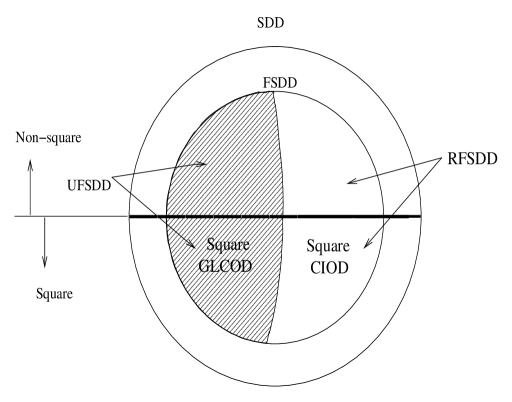
Figure 1: The classes of Full-rank Single-symbol Decodable Designs (FSDD).

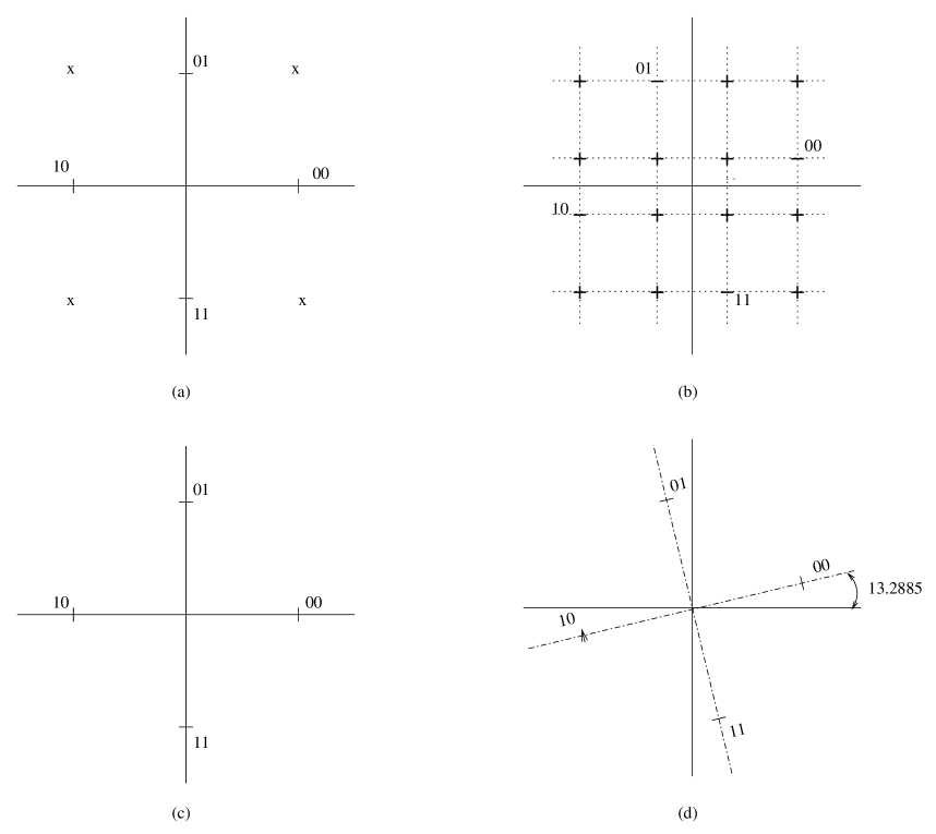
Figure 2: Expanded signal sets $\tilde{\cal A}$ for ${\cal A}=\{1,-1,{\mathbf{j}},-{\mathbf{j}}\}$ and a rotated version of it.

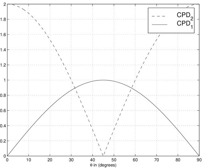
Figure 3: The plots of $CPD_{1},CPD_{2}$ for $\theta\in[0~{}90^{\circ}]$.

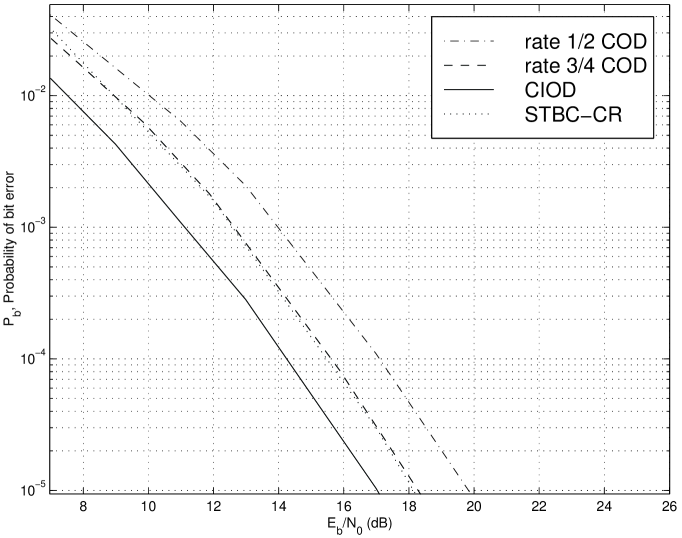
Figure 4: The BER performance of coherent QPSK rotated by an angle of $13.2825^{\circ}$ (Fig. 2) used by the CIOD scheme for 4 transmit and 1 receive antenna compared with STBC-CR, rate 1/2 COD and rate 3/4 COD at a throughout of 2 bits/sec/Hz in Rayleigh fading for the same number of transmit and receive antennas.

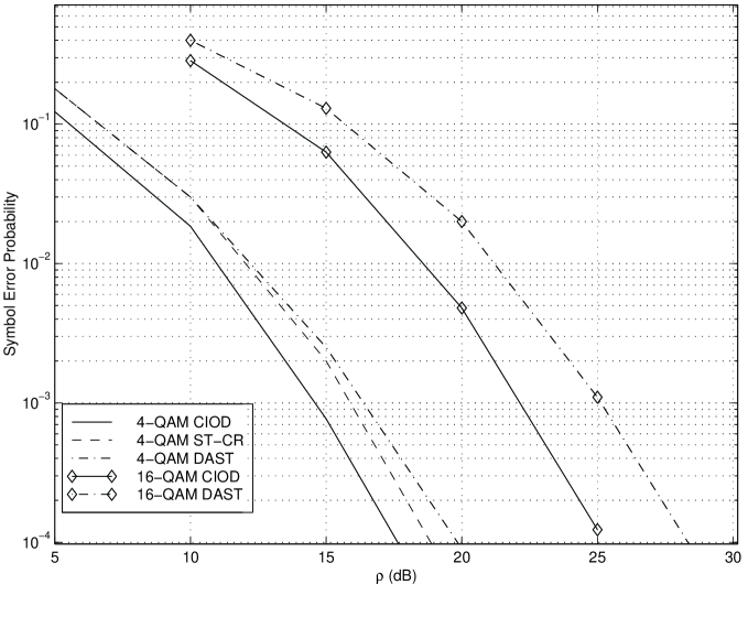
Figure 5: The BER performance of the CIOD with 4- and 16-QAM modulations and comparison with ST-CR and DAST schemes.

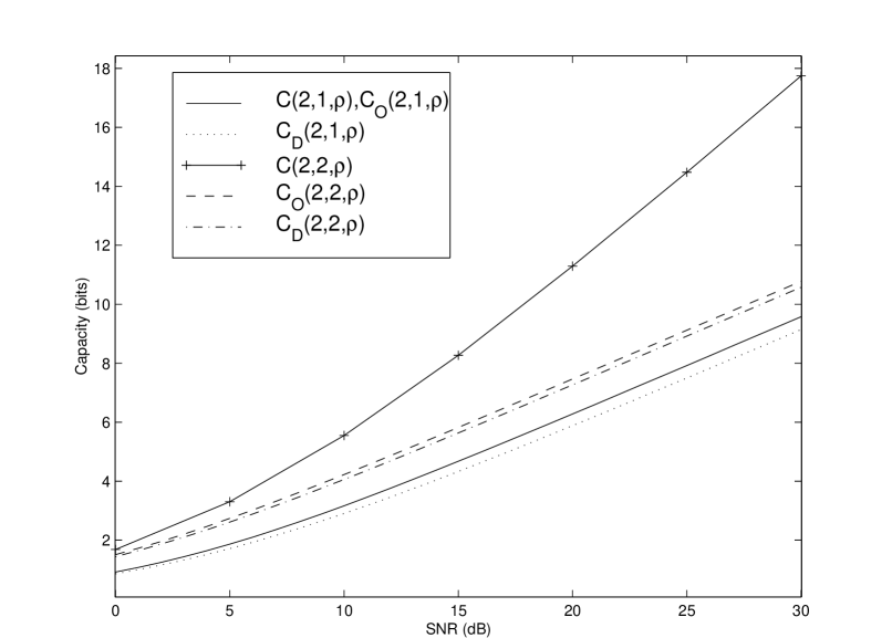
Figure 6: The maximum mutual information (ergodic) of CIOD code for two transmitters and one, two receivers compared with that of complex orthogonal design (Alamouti scheme) and the actual channel capacity.

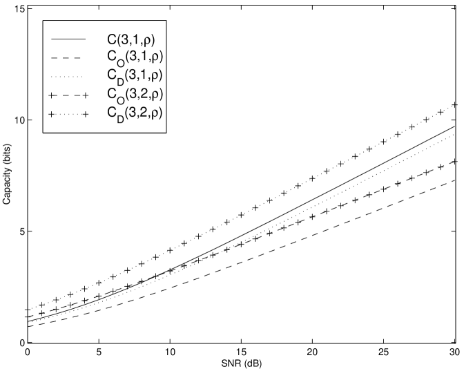
Figure 7: The maximum mutual information (ergodic) of GCIOD code for three transmitters and one, two receivers compared with that of code rate 3/4 complex orthogonal design for three transmitters and the actual channel capacity.

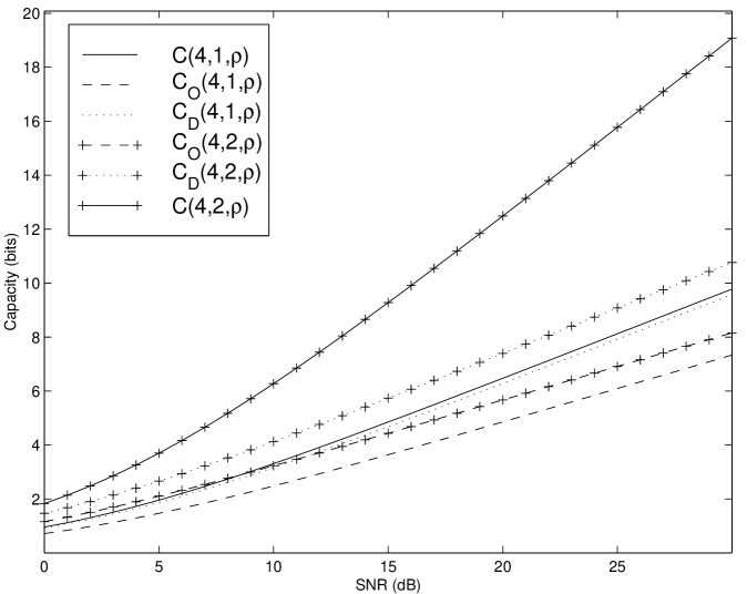
Figure 8: The maximum mutual information (ergodic) of CIOD code for four transmitters and one, two receivers compared with that of code rate 3/4 complex orthogonal design for four transmitters and the actual channel capacity.

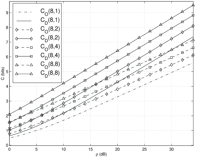
Figure 9: The maximum mutual information (average) of rate 2/3 GCIOD code for eight transmitters and one, two, four and eight receivers compared with that of code rate 1/2 complex orthogonal design for eight transmitters over Rayleigh fading channels.

Md. Zafar Ali Khan (S’00-M’06) was born in Hyderabad, India. He received the B.E. in electronics and communication from Osmania University, M.Tech. in electrical engineering from IIT, Delhi and Ph.D. in electrical communication engineering from IISc, Bangalore in 1996, 1998 and 2003 respectively. He was a design engineer with Sasken, Bangalore in 1999, a senior design engineer at insilica semiconductors, Bangalore, India from 2003 to 2005 and Sr. member of tech. staff at Hellosoft, India in 2005. He is presently with IIIT, Hyderabad as an Assistant Professor. His primary research interests are in coded modulation, space-time coding and signal processing for wireless communications.

B. Sundar Rajan (S’84-M’91-SM’98) was born in Tamil Nadu, India. He received the B.Sc. degree in mathematics from Madras University, Madras, India, the B.Tech degree in electronics from Madras Institute of Technology, Madras, and the M.Tech and Ph.D. degrees in electrical engineering from the Indian Institute of Technology, Kanpur, India, in 1979, 1982, 1984, and 1989 respectively. He was a faculty member with the Department of Electrical Engineering at the Indian Institute of Technology in Delhi, India, from 1990 to 1997. Since 1998, he has been a Professor in the Department of Electrical Communication Engineering at the Indian Institute of Science, Bangalore, India. His primary research interests are in algebraic coding, coded modulation and space-time coding. Dr. Rajan is a Member of the American Mathematical Society.

References

- [1] J. G. J. Foschini and M. J. Gans, “On limits of wireless communication in a fading environment using multiple antennas,” Wireless Personal Communication, Vol. 6, no. 3, pp. 311-335, Mar. 1998.
- [2] E. Teletar, “Capacity of multi-antenna Gaussian channels,” European Transactions on Telecommunications, Vol. 10, no. 6, pp. 585-595, Nov. 1999.
- [3] N. Seshadri and J. H. Winters, “Two signaling schemes for improving the error performance of FDD transmission systems using transmitter antenna diversity,” Int. Journal of Wireless Inform. Networks, Vol. 1, pp. 49-60, 1994.
- [4] J. Guey, M. P. Fitz, M. R. Bell, and W. Y. Kuo, “Signal design for transmitter diversity wireless communication systems over Rayleigh fading channels,” in Proc. of IEEE VTC 96, 1996, pp. 136–140.
- [5] V. Weerackody, “Diversity of direct-sequence spread spectrum system using multi transmit antennas,” in Proc. of IEEE ICC 93, 1993, pp. 1775-1779.
- [6] J. Winters, “Switched diversity with feedback for DPSK mobile radio systems,” IEEE Trans. Veh. Technol., Vol. VT-32, pp. 134-150, Feb. 1983.
- [7] ——, “Diversity gain of transmit diversity in wireless systems with Rayleigh fading,” in Proc. of IEEE ICC 94, Vol. 2, 1994, pp. 1121-1125.
- [8] V. Tarokh, N. Seshadri, and A. R. Calderbank, “Space-time codes for high data rate wireless communication: performance criterion and code construction,” IEEE Trans. Inform. Theory, Vol. 44, pp. 744-765, Mar. 1998.
- [9] V. Tarokh, H. Jafarkhani, and A. R. Calderbank, “Space-time block codes from orthogonal designs,” IEEE Trans. Inform. Theory, Vol. 45, pp. 1456-1467, July 1999.
- [10] V. Tarokh, H. Jafarkhani and A. R. Calderbank , “Correction to “Space-time block codes from Orthogonal designs”,”IEEE Trans. on Inform. Theory, Vol. 46, No.1, pp.314, Jan. 2000.
- [11] O. Tirkkonen and A. Hottinen, “Square matrix embeddable STBC for complex signal constellations,” IEEE Trans. Inform. Theory, Vol. 48, no. 2, pp. 384-395, Feb. 2002.
- [12] S. M. Alamouti, “A simple transmit diversity technique for wireless communications,” IEEE J. Select. Areas Commun., Vol. 16, no. 8, pp. 1451-1458, Oct. 1998.
- [13] G. Ganesan and P. Stoica, “Space-time diversity,” in Signal Processing Advances in Wireless and Mobile Communications, 2000, Vol. 1, Ch. 2, pp. 59-87.
- [14] ——, “Space-time block codes: a maximal SNR approach,” IEEE Trans. Inform. Theory, Vol. 47, no. 4, pp. 1650-1656, May 2001.
- [15] ——, “Space-time diversity using orthogonal and amicable orthogonal designs,” in Proc. of ICASSP 2000, Istanbul, Turkey, 2000, pp. 2561-2564.
- [16] X.-B. Liang and X.-G. Xia, “On the Nonexistence of Rate-One Generalized Complex Orthogonal Designs, ,” IEEE Trans. Inform. Theory,vol. 49, no. 11, Nov. 2003, pp. 2984-2988 .
- [17] X.-B. Liang, “Orthogonal Designs With Maximal Rates ,” IEEE Trans. Inform. Theory, Vol. 49, No. 10, pp.2468-2503, Oct. 2003.
- [18] W. Su and X.-G. Xia, “Two generalized complex orthogonal space-time block codes of rates 7/11 and 3/5 for 5 and 6 transmit antennas,” IEEE Trans. Inform. Theory, Vol. 49, pp. 313 -316, Jan. 2003.
- [19] ——, “On space-time block codes from complex orthogonal designs,” Wireless Personal Communications (Kluwer Academic Publishers), vol. 25, no. 1, pp.1-26, April 2003.
- [20] G. Ganesan, “Designing space-time codes using orthogonal designs,” Ph.D. dissertation, Uppsala University, Uppasal, Sweden, 2002.
- [21] H. Jafarkhani, “A quasi-orthogonal space-time block code,” IEEE Trans. Commun., Vol. 49, pp. 1-4, Jan. 2001.
- [22] O. Tirkkonen and A. Hottinen, “Complex space-time block codes for four Tx antennas,” in Proc. of Globecom 2000, pp. 1005-1009, Nov. 2000.
- [23] N. Sharma and C. B. Papadias, “Improved quasi-orthogonal codes through constellation rotation,” IEEE Trans. Commun., Vol. 51, no. 3, pp. 332–335, Mar. 2003.
- [24] ——, “Improved quasi-orthogonal codes,” in Proc. of IEEE WCNC 2002, pp. 169-171, Mar. 2002.
- [25] C. B. Papadias and G. J. Foschini, “A space-time coding approach for systems employing four transmit antennas,” in Proc. of IEEE ICASSP 2002, Vol. 4, 2002, pp. 2481-2484.
- [26] Weifeng-Su and X. Xia, “Quasi-orthogonal space-time block codes with full-diversity,” in Proc. of Globecom 2002, Vol. 2, Taipai, Taiwan, Nov. 2002, pp. 1098-1102.
- [27] W. Su and X.-G. Xia, “Signal constellations for quasi-orthogonal space-time block codes with full-diversity,” IEEE Trans. Inform. Theory, vol. 50, No. 10, Oct. 2004, pp. 2331-2347.
- [28] T. Josefiak, “Realization of Hurwitz-Radon matrices,” Queen’s papers on pure and applied mathmatics, no. 36, pp. 346-351, 1976.
- [29] A. V. Geramita and J. M. Geramita, “Complex orthogonal designs,” Journal of Combin. Theory, Vol. 25, pp. 211-225, 1978.
- [30] I. N. Herstein, Non-commutative rings, ser. Carus mathematical monograms. Washington DC, USA: Math. Assoc. Amer., 1968, Vol. 15.
- [31] A. V. Geramita and J. Seberry, Orthogonal designs, quadratic forms and Hadamard matrices, ser. Lecture Notes in Pure and Applied Mathematics. Berlin, Germany: Springer, 1979, Vol. 43.
- [32] Y. Xin, Z. Wang, and G. B. Giannakis, “Space-time constellation rotating codes maximizing diversity and coding gains,” in Proc. IEEE Globecom 2001, Vol. 1, Vancouver, Canada, Nov. 2001, pp. 455-459.
- [33] ——, “Linear unitary precoders for maximum diversity gains with multiple transmit and receive antennas,” in Proc. IEEE ASILOMAR 2000, Pacific Grove, USA, Nov. 2000, pp. 1553-1557.
- [34] M. O. Damen, K. Abed-Meraim, and J.-C. Belfiore, “Diagonal algebraic space-time block codes,” IEEE Trans. Inform. Theory, Vol. 48, no. 3, pp. 384-395, Mar. 2002.
- [35] M. O. Damen and N. C. Beaulieu, “On diagonal algebraic space-time block codes,” IEEE Trans. Commun., vol. 51, June 2003.
- [36] B. Hassibi and B. Hochwald, “High-rate codes that are linear in space and time,” IEEE Trans. Inform. Theory, Vol. 48, no. 7, pp. 1804–1824, July 2002.
- [37] S. Sandhu, “Signal design for MIMO wireless: a unified perspective,” Ph.D. dissertation, Stanford University, Stanford, CA, Aug. 2002.
- [38] M. O. Damen, K. Abed-Meraim, and J.-C. Belfiore, “Lattice codes decoder for space-time codes,” IEEE Commun. Lett., Vol. 4, pp. 161–163, May 2000.
- [39] ——, “Generalized sphere decoder for asymmetrical space-time communication architecture,” Electronics Letters, Vol. 36, no. 2, pp. 166–167, Jan. 2000.
- [40] S. B. Slimane, “An improved PSK scheme for fading channels,” IEEE Trans. Veh. Technol., Vol. 47, no. 2, pp. 703–710, May 1998.
- [41] ——, “An improved PSK scheme for fading channels,” in Proc. IEEE GLOBECOM ’96, Nov. 1996, pp. 1276–1280.
- [42] B. D. Jelicic and S. Roy, “Design of trellis coded QAM for flat fading and AWGN channel,” IEEE Trans. Veh. Technol., Vol. 44, pp. 192–201, Feb. 1995.
- [43] ——, “Cutoff rates for co-ordinate interleaved QAM over Rayleigh fading channel,” IEEE Trans. Commun., Vol. 44, no. 10, pp. 1231–1233, Oct. 1996.
- [44] D. Goeckel, “Coded modulation with non-standard signal sets for wireless OFDM systems,” in Proc. IEEE ICC 1999, Vol. 2, 1999, pp. 791–795.
- [45] A. Chindapol and J. Ritcey, “Bit-interleaved coded modulation with signal space diversity in Rayleigh fading,” in Proc. IEEE ASILOMAR 1999, Vol. 2, Pacific Grove, USA, Nov. 1999, pp. 1003–1007.
- [46] Md. Zafar Ali Khan and B. Sundar Rajan, “A co-ordinate interleaved orthogonal design for four transmit antennas,” IISc-DRDO Report, No. TR-PME-2002-17, Department of Electrical Communication Engineering, Indian Institute of Science, Bangalore, India, October 2002.
- [47] ——, “A co-ordinate interleaved orthogonal design for three transmit antennas,” in Proc. of National Conference on Communications , Mumbai, India, January 2002.
- [48] ——, “Space-time block codes from co-ordinate interleaved orthogonal designs,”in Proc. of ISIT 2002, pp. 316, Lausanne, Switzerland, June 30 - July 5, 2002.
- [49] Md. Zafar Ali Khan, B. Sundar Rajan and M. H. Lee, “On single-symbol and double-symbol decodable STBCs,” Proc. of ISIT 2003, Yokohama, Japan, June 29-July 3, 2003, pp.127.
- [50] Md. Zafar Ali Khan and B. Sundar Rajan, “Space-time block codes from designs for fast-fading channels,” Proc. of ISIT 2003, Yokohama, Japan, June 29-July 4, 2003, pp.154.
- [51] ——, “A Generalization of some existence results on Orthogonal Designs for STBCs,” to appear in IEEE Trans. Inform. Theory, Vol. 50, No. 1, Jan., 2004 pp.218-219.
- [52] ——, “Space-Time Block Codes from Designs for Fast-Fading Wireless Communication,” IISc-DRDO Technical Report, No: TR-PME-2003-07, Department of Electrical Communication Engineering, Indian Institute of Science, Bangalore, India, May 2003.
- [53] B. Sundar Rajan, Md. Zafar Ali Khan and M. H. Lee, “A co-ordinate interleaved orthogonal design for eight transmit antennas,” IISc-DRDO Report, No. TR-PME-2002-16, Department of Electrical Communication Engineering, Indian Institute of Science, Bangalore, India, October 2002.
- [54] Zafar Ali Khan, B. Sundar Rajan and H.H.Lee “Rectangular Coordinate Interleaved Orthogonal Designs,” Proceedings of IEEE GLOBECOM 2003, Communication Theory Symposium, San Francisco, Dec. 2003, Vol.4, pp.2004-2009.
- [55] Md. Zafar Ali Khan and B. Sundar Rajan, “Bit and co-ordinate interleaved coded modulation,” in Proc. IEEE GLOBECOM 2000, San Francisco, USA, Nov. 2000, pp. 1595–1599.
- [56] Md. Zafar Ali Khan, “Single-symbol and Double-symbol Decodable STBCs for MIMO fading channels,” Ph.D. Thesis, Indian Institute of Science, Bangalore, India, July 2003.
- [57] Chau Yuen, Yong Liang Guan and T. T. Tjhung,“Construction of Quasi-orhogonal STBC with Minimum Decoding Complexity from Amicable Orthogonal Designs,” Proc. of ISIT 2004, Chicago, USA, June 29-July 3, 2004.
- [58] Chau Yuen, Yong Liang Guan and T. T. Tjhung,“Quasi-Orthogonal STBC with Minimum Decoding Complexity: Further Results,” Proc. of WCNC 2005, USA, pp. 483-488.
- [59] Haiquan Wang, Dong Wang, and Xiang-Gen Xia, “On Optimal Quasi-Orthogonal Space-Time Block Codes with Minimum Decoding Complexity,” Proc. of ISIT 2005, pp. 1168-1172.
- [60] K. Boull and J. C. Belfiore,“Modulation scheme designed for Rayleigh fading channel”, presented at CISS’92, Princeton, NJ, March 1992.
- [61] J. Boutrous, E. Viterbo, C. Rastello and J. C. Belfiore, “Good lattice constellationsfor both Rayleigh fading and Gaussian channel,” IEEE Trans. Inform. Theory, Vol.42, pp. 502–518, March 1996.
- [62] J. Boutrous and E. Viterbo, “Signal space diversity: a power and bandwidth efficient diversity technique for Rayleigh fading channel,” IEEE Trans. Inform. Theory, Vol. 44, no. 4, pp. 1453–1467, July 1998.
- [63] Z. Chen, J. Yuan, and B. Vucetic, “An improved space-time trellis coded modulation scheme on slow Rayleigh fading channels,” in Proc. IEEE International Conference on Communications 2001, Vol. 4, Helsinki, Finland, June 2001, pp. 1110–1116.
- [64] Mohammed Ali Maddah-Ali and Amir K. Khandani,“A new non-orthogonal space-time code with low decoding complexity,” private communication.
- [65] R.A.Horn and C.R.Johnson, Matrix Analysis, Cambridge University Press, 1985.