Parameter Estimation of Hidden Diffusion Processes: Particle Filter vs. Modified Baum-Welch Algorithm

Abstract

We propose a new method for the estimation of parameters of hidden diffusion processes. Based on parametrization of the transition matrix, the Baum-Welch algorithm is improved. The algorithm is compared to the particle filter in application to the noisy periodic systems. It is shown that the modified Baum-Welch algorithm is capable of estimating the system parameters with better accuracy than particle filters.

1 Introduction

Identification or parameter estimation is one of the most important and interesting fields in the nonlinear dynamics and time series analysis. There exist many methods of identifying the parameters of a nonlinear stochastic system such as maximum Likelihood estimators and Bayes estimators [1]. Especially this latter is related to the Sequential Monte Carlo methods [2] which are also known as Particle filter methods introduced by Gordon et al. [3]. These methods utilize a large number of random samples (or particles) to represent the posterior probability distributions. The particles are propagated over time using a combination of sequential importance sampling and resampling steps. At each time step the resampling procedure statistically multiplies and/or discards particles to adaptively concentrate particles in regions of high posterior probability.
Particle filter methods are usually applied to state space models to approximate the posterior probability distributions of the state given the available observation. If the state space models contain a set of unknown parameters which are to be estimated then one can include them in the model by augmenting the state vector [4].
As an alternative method for estimating parameters of continuous hidden diffusion processes we propose a hidden Markov models (HMMs) [5] approach which model both the signal and noise simultaneously [6]. This is based on the approximation of continuous systems by discrete models. The underlying signal is assumed to be generated by a discrete Markov chain. The latter uses the joint probability of the sequence of the discrete observation samples as the likelihood function. The general theory of HMMs was established by Baum et al. in the sixties [7, 8, 9].
Standard HMMs rely on the Baum-Welch reestimation procedure to optimize the likelihood function [5]. The standard Baum-Welch algorithm suffers from the problem that it may converge to a local minimum. However, we can overcome this difficulty by parameterizing the transition matrix [10].
Previous works have shown that hidden Markov models are successful tools for modeling and classifying dynamic behaviors. For example, HMMs are used for analyzing biological sequences [11], speech recognition [12], ion channel analysis [13, 14, 15], and to detect different modes of neuronal activity [16].
In experimental physics, the objective of any measurement is to determine the value of the particular quantity to be measured. In general, however, the result of a measurement is only an approximation or estimate of the value one is looking for. For instance in coupled Josephson junctions [17], direct measurements of the time dependence of the voltage are usually impossible because the characteristic time scale of voltage variations is too short ($\sim$ picoseconds). One can usually measure the Josephson radiation emission in some narrow frequency range, which can show chaotic behaviour. But in this case one cannot see higher harmonics which are required to fully reconstruct the voltage time evolution. In experiments, another version of the voltage is usually measured which is the results of the low pass filtering. The obtained voltage is used to extract the current-voltage characteristic. In this case, the observed variable is the voltage whereas the Josephson phase is hidden. Likharev [17] reported that the coupled Josephson junctions belong to a class of complex systems. The corresponding experimental works show that it is difficult to estimate some of the parameters characterizing the Josephson device, e.g. the damping related to the fluctuation of the temperature and the maximal Josephson current.
For the case that the measured time series proved to be approximately Markovian, Friedrich et al [18, 19] proposed an approach to obtain the drift and diffusion of one-dimensional Langevin equations from the time series. This is based on the finite-difference form of their definition together with suitable interpolations of the resulting trends. Ragwitz et al. [20] proposed a correction of this approach to reduce the errors due to a finite times step. This was controversy for the case of directly observed states of continuous diffusion processes, which were measured in discrete time [20], [19], [21]. We believe that our approach can then be used to clarify this situation.
This paper is devoted to a numerical evaluation of these two methods by applying them, for instance, to the problem of diffusion in periodic potentials with noisy observations. The latter example is taken as a periodic function of the coordinate of the diffusing state. The aim of this work is to estimate the drift coefficient and the diffusion constant.
The paper is organized as follows. In the next section, we formulate the problem of hidden diffusion processes. In section 3, we review the particle filter and propose a modified Baum-Welch algorithm. Section 4 is devoted to a numerical simulation and the evaluation of both methods. Conclusions are given in the last section.

2 Mathematical model

Diffusion processes are usually modeled by the evolution equation of the probability density function ${\mathcal{P}}$ which is governed by the continuous Fokker-Planck equation. This can be read in one dimension

$$\frac{\partial}{\partial t}{{\mathcal{P}}}(x,t)=-\frac{\partial}{\partial x}\left[F(x){{\mathcal{P}}}(x,t)\right]+{1\over 2}\frac{\partial^{2}}{\partial x^{2}}\left[D(x){{\mathcal{P}}}(x,t)\right]\;,$$ (1)

where $F$ is the drift and $D$ is the diffusion coefficient. The process of Eq. (1) can equivalently be described by a Langevin equation interpreted in Itô sense

$$\dot{x}=F(x)+\sqrt{D(x)}\,v(t)\;,$$ (2)

where $v(t)$ is intrinsic white noise with the density $q(v_{t})$, and the initial condition of Eq. (2) is given by $x(t=0)~{}\sim\mu(x(0))$.
The state variable $x(t)$ can usually not be observed directly but only via a measurement process, which is modeled by an observation function $h$ as

$$y(t)=h(x(t),w(t))\;,$$ (3)

where $w(t)$ denotes observation noise with the density $r(w_{t})$ which is independent of $v(t)$.
Eq. (2) together with Eq. (3) define hidden diffusion processes.
In general, the observation function $h$ is nonlinear. Thus, the diffusing state $x$ is hidden. The estimation problem therefore becomes difficult to tackle and there exists no analytical method dealing with diffusion coefficient estimation. There exist only approximate numerical methods such as particle filters. In practice, the particle filters are applied to discretized version of the system (2–3), which result in the state space model

$$x_{t} = G_{t}(x_{t-1},v_{t})$$ (4)

$$y_{t} = H_{t}(x_{t},w_{t})\,,$$ (5)

where $G_{t}$ and $H_{t}$ are assumed to be known nonlinear functions, the dynamical white noise $v_{t}$ and the observation white noise $w_{t}$ are independent random processes and the initial condition $x_{0}\sim p(x_{0})$.
In the next section, we give a short overview of the particle filters and the corresponding implementation issues (more details can be found in [3, 2, 22, 23]).
We assume that the diffusion coefficient $D(x)=D$ is constant throughout the paper.

3 Algorithms

3.1 Particle filter algorithm (Monte Carlo Filter)

Consider systems that are described by the generic state space model (4–5). Sequential Monte Carlo methods or particle filters provide an approximate Bayesian solution to the discrete time recursive of the state space model (4–5) by updating an approximate description of the posterior filtering density.
Let $x_{t}$ denote the state of the observed system and ${\mathcal{Y}}_{t}=\{y_{i}\}_{i=1}^{t}$ the set of observations up to the present time $t$. Let the independent process noise $v_{t}$ and the measurement noise $w_{t}$ with the densities $q(v_{t})$ respective $r(w_{t})$. The initial uncertainty is described by the density $p(x_{0})$. The particle filter approximates the probability density $p(x_{t}|{\mathcal{Y}}_{t})$ by using a large set of $N_{p}$ particles $\{x^{(i)}_{t}\}_{i=1}^{N_{p}}$, where each particle has an assigned relative weight $m^{(i)}_{t}$, such that all weights sum to one. The particle filter updates the particle location and the corresponding weights recursively with each new observation. The non-linear prediction density $p(x_{t}|{\mathcal{Y}}_{t-1})$ and optimal filtering density $p(x_{t}|{\mathcal{Y}}_{t})$ for the Bayesian interference are given by

$$p(x_{t}|{\mathcal{Y}}_{t-1}) = \int p(x_{t}|x_{t-1})p(x_{t-1}|{\mathcal{Y}}_{t-1}){\rm d}x_{t-1}$$ (6)

$$p(x_{t}|{\mathcal{Y}}_{t}) = \frac{p(y_{t}|x_{t})\,p(x_{t}|{\mathcal{Y}}_{t-1})}{p(y_{t}|{\mathcal{Y}}_{t-1})}\;,$$ (7)

where $p(y_{t}|{\mathcal{Y}}_{t-1})=\int p(y_{t}|x_{t})p(x_{t}|{\mathcal{Y}}_{t-1}){\rm d}x_{t}$. The transition probability density $p(x_{t}|x_{t-1})$ is know as the motion model (4) and $p(x_{t-1}|{\mathcal{Y}}_{t-1})$ is the updated estimate from the previous step. $p(y_{t}|x_{t})$ is the observation probability density given by Eq. (5).
Note that, generally, these equations are not analytically tractable. However, for the important special case of linear dynamics, linear measurements and Gaussian noise there exist a closed form solution of Eq.(6–7) , given by the Kalman filter [24].
The main idea of the optimal filter is to approximate $p(x_{t}|{\mathcal{Y}}_{t-1})$ with

$$p(x_{t}|{\mathcal{Y}}_{t-1})\approx{1\over N_{p}}\sum_{i=1}^{N_{p}}\delta(x_{t}-x^{(i)}_{t})\,,$$ (8)

where $\delta$ is the Dirac delta distribution.
Inserting (8) into (7) yields a density of a simple form. This can be done by using the Bayesian bootstrap or Sampling Importance Resampling (SIR) algorithm from [2] which is given by the following algorithm

1. At $t=0$, generate random numbers $x_{0}^{(j)}\sim p(x_{0})\,{\sf for}\,j=1,...,N_{p}$ 2. Repeat the following steps for $t=1,...,T$ (a) Generate random numbers $v_{t}^{(j)}\sim q(v)\,{\sf for}\,j=1,...,N_{p}$ (b) Compute $p_{t}^{(j)}=G(x_{t-1}^{(j)},v_{t}^{(j)})\,{\sf for}\,j=1,...,N_{p}$ (c) Compute $m_{t}^{(j)}=p(y_{t}|p_{t}^{(j)})\,{\sf for}\,j=1,...,N_{p}$ (d) Resample with replacement $N_{p}$ particles $\{x_{t}^{(j)}\}$ from $\{p_{t}^{(j)}\}$ according to the importance weights

Table 1: Particle filter algorithm

Note that the resampling procedure (step (2d) in the Table 1) selects only the fittest particles to obtain an unweighted measure $\{(x_{t}^{(j)},\frac{1}{N_{p}}\}$.
Sometimes the resampling step is omitted and simply imposed when needed to avoid a divergence in the particle filter as in the sequential importance sampling (SIS) method, where the weight is updated recursively as [23]

$$m_{t}^{(j)}=m_{t-1}^{(j)}\cdot p(y_{t}|p_{t}^{(j)})\,{\sf for}\,j=1,...,N_{p}$$

As the estimate of the state we choose the minimum mean square estimate, i.e.

$$\hat{x}_{t}=\int x_{t}p(x_{t}|{\mathcal{Y}}_{t}){\rm d}x_{t}\approx\sum_{i=1}^{N_{p}}\tilde{m}^{(i)}_{t}x^{(i)}_{t}\,.\\$$ (9)

where $\tilde{m}^{(i)}_{t}={m}^{(i)}_{t}/\sum_{i=1}^{N_{p}}{m}^{(i)}_{t}$.

Parameter estimation: the state space model (4–5) usually contains several unknown parameters, such as the variances of the noises and the coefficients of the functions $F_{t}$ and $H_{t}$. Let us denote such unknown parameters by ${\theta}=(\theta_{0},\cdots,\theta_{N_{\theta}})$. We consider a Bayesian estimation problem by augmenting the state vector $x_{t}$ with the unknown parameter vector ${\theta}$ as

$$z_{t}=\left[\begin{array}[]{l}x_{t}\\ {\theta_{t}}\end{array}\right]\,,$$ (10)

with $\dot{{\theta}_{t}}=0$. The state space model for this augmented state vector $z_{t}$ is thus

$$\begin{array}[]{ll}z_{t}=G^{*}_{t}(z_{t-1},v_{t})\\ y_{t}=H^{*}_{t}(z_{t},w_{t})\quad,\end{array}$$ (11)

where the nonlinear functions $G^{*}_{t}(z,v)=(G_{t}(x,v),\theta_{t})$ and $H^{*}_{t}(z,w)=H_{t}(x,w)$. We can therefore apply the particle filter algorithm to the state space models described by Eq. (11) as previously.

3.2 HMM and Modified Baum-Welch algorithm

The approximation of continuous hidden diffusion processes (2)–(3) by discrete models results in Hidden Markov Models (HMMs). In [10] the diffusion process was approximated by a discrete random walk with $N$ states with only nearest neighbor transitions. For the observation process we considered an appropriate discrete process, which is well defined in the continuous time limit, e.g. consider Eq. (3) in discrete form.
Comparing Fokker-Planck equations on the one hand with discrete time and space master equations on the other hand, it is easy to establish the connection between the continuous diffusion process and the Markov model parameters as in [10]

$$F(i\,\Delta x) = {{a_{i,i+1}-a_{i,i-1}}\over\Delta x}D_{0}$$ (12)

$$D(i\,\Delta x) = [(a_{i,i+1}+a_{i,i-1})-(a_{i,i+1}-a_{i,i-1})^{2}]D_{0}\,,$$

where $D_{0}={{\Delta x}^{2}\over{\Delta t}}$ and $a_{i,j}$ are the elements of the transition matrix. The continuum limit ${\Delta x},{\Delta t}\rightarrow 0$ can be approached by keeping $D_{0}$ constant.
Relations (12–LABEL:da) are important, because they give a justification for the approximation of continuous diffusion processes by discrete models.
Standard HMMs rely on standard Baum-Welch reestimation procedure to optimize the likelihood function (more details can be found in [10]). The procedure may have several drawbacks if it is applied to the problem of diffusion in periodic potentials with noisy observations. Since the observation function was simply chosen as the cosine of the state variable, the maxima of likelihood function are degenerate e.g. each state is observed with two different observations. More importantly, in order to converge to the continuous hidden diffusion processes, we should choose a large number of states, which means that many parameters should be re-estimated. In this case, the standard Baum-Welch algorithm is not applicable, due to the limited number of observations. To avoid these problems we have to use a modified version of the Baum-Welch algorithm . It consists in parameterizing the matrix of the transition probability. For instance, this can be done by a Fourier expansion of the elements of the transition matrix.

$$\{a_{k,k+j}\}=\{a_{k,k+j}({\theta})\}=\sum_{n=0}^{N-1}\theta_{n}(j)exp\left(i\,2\pi\,\frac{kn}{N}\right)\qquad{\rm for}\,j=-1,1\;,$$ (14)

Following [25] we obtain $N_{\theta}$ nonlinear implicit equations

$$\sum_{i\neq j}\frac{\partial a_{ij}({\theta}^{(n+1)})}{\partial\theta_{\kappa}^{(n+1)}}\left(\frac{\Psi_{ij}({{\mathcal{Y}}}_{t},\{a_{ij}({\theta}^{(n)})\})}{a_{ij}({\theta}^{(n+1)})}-\frac{\Psi_{ii}({{\mathcal{Y}}}_{t},\{a_{ii}({\theta}^{(n)})\})}{a_{ii}({\theta}^{(n+1)})}\right)=0\;,$$ (15)

for $\kappa=1,\cdots,N_{\theta}$.
The calculation of the conditional probability $\Psi_{ij}({{\mathcal{Y}}}_{t},\{a_{ij}({\theta}^{(n)})\})$ at iteration $n$ can be carried out by using the forward-backward algorithm given in [5].
In case of homogeneous random walks we derived in [10] an explicit expression for the new estimates of the parameterized transition probabilities in terms of previous estimates and the observed signal. In general, Eq. (15) has to be solved numerically, for example, by using the Newton methods. Then one can find the fixed point ${\theta}^{*}$ solution of Eq. (15).
Given a set of observation data ${{\mathcal{Y}}}_{t}=\{y\}_{t=1}^{t}$, the core of the modified Baum-Welch algorithm reads

1. Generate a hidden Markov model “trainer” with $N$ states and $M$ distinct observation symbols (a) Generate a tridiagonal transition matrix according to Eq. (14) (b) The observation matrix is given by the time discretization of Eq. (3) 2. Repeat until $\left|\log P(\vec{y}|a_{ij}({\theta}^{(n)})-\log P(\vec{y}|a_{ij}({\theta}^{(n-1)})\right|\leq 10^{-6}$ (a) Compute the conditional probability $\Psi_{ij}({{\mathcal{Y}}}_{t},\{a_{ij}({\theta}^{(n)})\})$ using the forward-backward algorithm given in [5] (b) Update the elements of the transition matrix using the formula (15)

Table 2: Combined HMM and modified Baum-Welch algorithm

An obvious advantage of the modified Baum-Welch algorithm is that it is independent of the number of states $N$ but depends only on the number of Fourier coefficients.

4 Simulation Results

We now present a simple example to illustrate the central ideas in this paper. We consider the system

$$\dot{X}_{t} = \left(\theta_{0}+\sum_{n=1}^{N_{\theta}}\theta_{n}\sin(2n\pi X_{t}/L)\right)\,+\sqrt{D}\,v_{t}$$ (16)

$$Y_{t} = (\cos(2\pi X_{t}/L))+\sqrt{\sigma}\,w_{t}\,,$$ (17)

with the initial condition $X_{0}\sim{\mathcal{N}}(0,1)$. The driving noise $v_{t}$ and the observation noise $w_{t}$ are independent Gaussian random processes of variance one. In Eq.(16–17), $L$ is the spatial extension (period) equal to $N\Delta x$ ( $N$ is the number of states of the discrete model) and ${\theta}=(\theta_{0},\cdots,\theta_{N_{\theta}},D)$ is the set of parameters to be estimated. Eq. (17) describes the observation processes.
For a practical implementation of the particle filter and the modified Baum-Welch algorithm, the necessary sample paths and stochastic integrals must be discretely approximated. Appropriate numerical methods are discussed by Klöden and Platen [26]. The Euler scheme is used here for this aim.
Once the observation sequence is generated by the model (16–17), we apply the two algorithms to reestimate the drift term and the diffusion constant.
Note that the application of particle filters in estimating parameters requires regarding the set of parameters ${\theta}$ as time dependent. That is, we have to consider a different model in which ${\theta}$ is replaced by ${\theta}_{t}$ at time $t$, and to include ${\theta}_{t}$ in the augmented state vector. Then we add an independent, zero-mean normal increment to the parameters at each time step. As a result, the discretized equations of system (16–17) read

$$\begin{array}[]{llll}x^{t}&=x^{t-1}+\left(\theta_{0}^{t-1}+\sum_{n=1}^{N_{\theta}}\theta_{n}^{t-1}\sin(2n\pi X_{t}/L)\right)\Delta t+\theta_{N_{\theta}+1}^{t-1}v_{t}\\ \theta_{n}^{t}&=\theta_{n}^{t-1}+u^{t}_{n}\quad{\rm for}\quad n=0,1,\cdots,N_{\theta}+1\\ y_{t}&=\cos(2\pi x^{t}/L)+\sqrt{\sigma}\,w_{t}\,,\end{array}$$ (18)

where ${\left(\theta_{N_{\theta}+1}^{t}\right)}^{2}=D_{t}$, $v_{t}\sim{\mathcal{N}}(0,\sqrt{\Delta t})$, $u^{t}_{n}\sim{\mathcal{N}}(0,\epsilon\sqrt{\Delta t})$ and $w_{t}\sim{\mathcal{N}}(0,1)$.

For simplicity, we restrict ourselves to the case $N_{\theta}=1$ and $\Delta t=1$.
In order to compare the numerical results given by the particle filter with the modified Baum-Welch algorithm we consider the drift parameters $\theta_{0}=-0.1$, $\theta_{1}=0.1$, the diffusion constant $D=0.8$ and we assume that there is no observation noise $\sigma=0$.
First, the particle filter is applied to the entire augmented state vector, using the scheme of Table 1. The initial value and the initial covariance of the estimated augmented state vector (18) we were set to

$$\left(\begin{array}[]{cc}\hat{x}^{0}\\ \hat{\theta}^{0}_{0}\\ \hat{\theta}^{0}_{1}\\ \hat{\theta}^{0}_{2}\\ \end{array}\right)=\left(\begin{array}[]{cc}1\\ 0\\ 0\\ 0\\ \end{array}\right),\qquad P^{0}=\left(\begin{array}[]{cccc}5^{2}&0&0&0\\ 0&.1^{2}&0&0\\ 0&0&.1^{2}&0\\ 0&0&0&.1^{2}\\ \end{array}\right)\;.$$ (19)

The actual initial value of the state vector was drawn randomly from ${\mathcal{N}}(0,P^{0})$.

Figure 1: State $x$ (top left panel), parameter $\theta_{0}$ (top right panel), parameter $\theta_{1}$ (bottom left panel) and diffusion coefficient $D$ (bottom right panel) vs. time. The correct values are shown by solid black lines and the estimated values after applying the particle filter algorithm are represented by solid red lines.

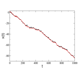
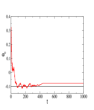
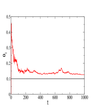
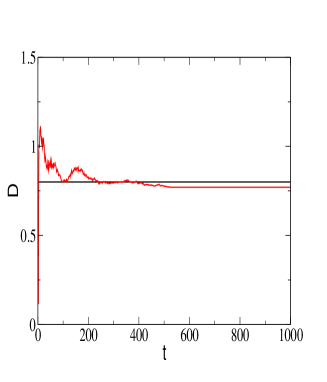
Fig. 1 shows the true state $x$, the parameters $\theta_{0}$, $\theta_{1}$ and the diffusion coefficient $D$ as a function of time and represent it as black solid lines. The values estimated from $N_{p}=1000$ are shown by red solid lines. After convergence, the particle filter gives a “reasonable” estimation for the state and better estimate of the correct values of the drift parameters $(\theta_{0},\theta_{1})$ and the diffusion constant $D$. However, the estimate state $x$ does not totally agree with the true values.
Note in Fig. 1 the stochastic character of the particle filter (because it is based on Monte Carlo methods).

Figure 2: Probability density function given by the particle filter algorithm

Fig. 2 presents the estimated filtering distributions. One can clearly see from this figure the multimodal non-Gaussian posterior distribution character.
Moreover, Tables 3 and 4 show the performance of the particle filters as function of the number of particles for two lengths of observation, $T=100$ and $T=1000$. More specifically, each table shows how many runs out of a total of 100 simulations diverged.

T=100

Number of particles	100	500	1000
$\theta_{0}$	92%	73%	43%
$\theta_{1}$	88%	74%	45 %
$D$	91%	76%	48 %

Table 3: Percentage of diverged runs of the estimated parameters for the particle filter.

T=1000

Number of particles	100	500	1000
$\theta_{0}$	89%	25%	5%
$\theta_{1}$	86%	25%	6%
$D$	90%	69%	10%

Table 4: Percentage of diverged runs of the estimated parameters for the particle filter.

One clearly sees from tables that it takes many particles and a large number of iterations for the particle filter to work well. The main reason for this is well known the degeneracy of particle filter if the process noise has a small variance [23].

In order to use a discrete HMM, we must first quantize the observation data into a set of standard vectors according to Elliott [6]. The quantized data are used as training sets for a HMM which has to learn the correct parameters from these observations.
Here, we  have  implemented  the  modified Baum-Welch algorithm described in Table 2. More details on implementation issues can be found in [10].

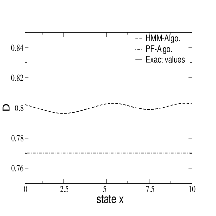
Fig. 3 shows the drift function and diffusion constant as a function of the coordinate $x$. The estimated values are represented as dot-dashed lines after applying the particle filter and as dashed lines for the modified Baum-Welch algorithm.
One can see from this figure that a convergence of the modified Baum-Welch algorithm to the correct parameter values was obtained. Moreover, the convergence is very fast, $n\approx 15$ ($n$ is the number of iterations), whereas the particle filter algorithm needs a large number of particles, $N_{p}=1000$, and needs larger number of iterations (around $500$) until convergence is obtained. Therefore, the time consuming is more relevant for the particle filter algorithm than for the modified Baum-Welch algorithm.

Figure 3: Drift F(x) (left panel) and diffusion coefficient $D$ (right panel) vs. the state. The correct parameters for the drift are $\theta_{0}=-0.1$ and $\theta_{1}=0.1$, and for the diffusion $D=0.8$ which are shown by solid lines. The estimated values given by the modified Baum-Welch algorithm are shown by dashed lines and the estimated values given by particle filter are represented by dot-dashed lines.

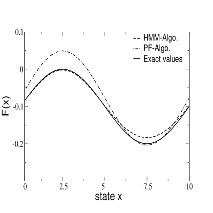
Note in Fig. 3 that using the modified Baum-Welch algorithm, the estimation of the drift function is better in the interval $x\leq 5$, whereas, it is better in the domain $x>5$ for the particle filter. This is the inverse situation if we choose another initial condition.

5 Conclusion

In this paper, we have proposed a modified Baum-Welch algorithm based on a parametrization of the transition matrix associated with HMMs. This algorithm has been compared to particle filters with the aim to reestimate the parameters of hidden diffusion processes in periodic potentials and, more precisely, to estimate the drift coefficient and the diffusion constant of periodic stochastic systems.
Our simulations show the following results: The particle filter algorithm, where the number of samples and the length of observation are chosen to be large $(N_{p}=1000,\,T=1000)$, converges quantitatively to the correct values of the drift and diffusion coefficients. The great advantage of the particle filter algorithm is its enormous flexibility. It can be applied to practically all nonlinear and/or non-Gaussian high-dimensional state space models within a statistical framework. This algorithm, however, is stochastic in nature (based on Monte Carlo) and, it requires a relatively large number of samples to ensure a fair maximum likelihood estimate of the current state. In contrast, the modified Baum-Welch algorithm is deterministic and the transition probabilities between the hidden states are constrained by the parametrization. The modified Baum-Welch algorithm converges to the correct results within 20-30 iterations of the reestimation procedure. Thus, the basic idea of this paper works well and the performance in large $N$ (continuum limit) can also be evaluated also for more complicated situations.

References

- [1] G. Casella, J. O. Berger, Statistical inference, Duxbury, 2nd edition, 2001.
- [2] G. Kitagawa, Monte Carlo filter and smoother non-Gaussian nonlinear filter state space models, J. Computation and Graphical Statistics, 5, 1–25 (1996).
- [3] N. J. Gordon, D. J. Salmond, A. Smith, Novel approach to nonlinear/non-Gaussian Bayesian state estimation, IEE-Proceedings-F, 140, 107–113 (1993).
- [4] J. Liu, M. West, Combined parameter and state estimation in simulation-based filtering, In Sequential Monte Carlo Methods in Practice, 197–223 (2001).
- [5] L. Rabiner, A tutorial on hidden Markov models and selected applications in speech recognition, Proc. IEEE, 77, 257–286 (1989).
- [6] R. J. Elliott, L. Aggoun, J. Moore, Hidden Markov Models: Estimation and Control, New York, 1995.
- [7] L. Baum, T. Petrie, Statistical inference for probabilistic functions of finite state Markov chains, Ann. Math. Statist., 37, 1554–1563 (1966).
- [8] L.E. Baum and J.A. Eagon; An Inequality with Applications to Statistical Estimation for Probabilistic Functions of Markov Processes and to a Model for Ecology. Bull. Amer. Math. Soc., 73, 360–363 (1967).
- [9] L.E. Baum, T. Petrie, G. Soules and N. Weiss; A Maximization Technique Occurring in the Statistical Analysis of Probabilistic Functions of Markov Chains. Ann. Math. Statist., 41, 164–171 (1970).
-
[10]
A. Benabdallah, A. Löser, G. Radons, From hidden diffusion processes to
hidden Markov models, Tech. rep., Preprint series of the DFG-SPP (December
2004).
URL http://www.math.uni-bremen.de/zetem/DFG-Schwerpunkt/preprints/prep066.pdf - [11] R. Durbin, S. Eddy, A. Krogh, G. Mitchison, Biological Sequence Analysis, Cambridge University Press, 2001.
- [12] L. R. Rabiner, B. H. Juang, Fundamentals of Speech Recognition, Engewood Cliffs, NJ: Prentice-Hall, 1993.
- [13] S. Chung, J. B. Moore, L. Xia, L. S. Premkumar, P. W. Gage, Characterization of single channel currents using digital signal processing techniques based on hidden Markov models, Phil. Trans. R. Soc. Lond. B, 329, 265–285 (1990).
- [14] D. R. Fredkin, J. A. Rice, Maximum likelihood estimation and identification directly from single-channel recording, Proc. R. Soc. Lond. B, 249, 25–132 (1992).
- [15] J. Becker, J. Honerkamp, J. Hirsch, U. Fröbe, E. S. r, R. Greger, Analyzing ion channels with hidden Markov models, Pflügers Arch., 426, 328–332 (1994).
- [16] G. Radons, J. D. Becker, B. Dülfer, J. Krüger, Analysis, classification, and coding of multi-electrode spike trains with hidden Markov-models, Biol. Cybern., 71, 359–373 (1994).
- [17] K. Likharev, Dynamics of Josephson Junctions and Circuits, Gordon and Breach Science Publishers, 1986.
- [18] S. Siegert, R. Friedrich, J. Peinke, Analysis of data sets of stochastic systems, Phys. Lett. A, 243, 275–280 (1998).
- [19] R. Friedrich, C. Renner, M. Siefert, J. Peinke, Comment on “indispensable finite time corrections for Fokker-Planck equations from time series data”, Phys. Rev. Lett., 89, 14901 (2002).
- [20] M. Ragwitz, H. Kantz, Indispensable finite time corrections for Fokker-Planck equations from time series data, Phys. Rev. Lett., 87, 254501 (2001).
- [21] M. Ragwitz, H. Kantz, Ragwitz and Kantz reply, Phys. Rev. Lett., 89, 149402 (2002).
- [22] M. Arulampalam, S. Maskell, N. Gordon, T. Clapp, Tutorial on particle filters for online nonlinear/non-Gaussian Bayesian tracking, IEEE Trans. Signal Process., 50, 174–188 (2002).
- [23] A. Doucet, N. D. Freitas, N. J. Gordon, in: Sequential Monte Carlo Methods in Practice, Springer, New York, 2001.
- [24] R. E. Kalman, A new approach to linear filtering and prediction problems, Trans. AMSE, J. Basic Engineering, 82, 35–45 (1960).
- [25] S. Michalek, J. Timmer, Estimating rate constants in hidden Markov models by the EM algorithm, IEEE Trans. Signal Processing, 47, 226–228 (1999).
- [26] P. E. Klöden, E. Platen, Numerical Solution of Stochastic Differential Equations, Springer, New York, 1999.