Trellis Pruning for Peak-to-Average Power Ratio Reduction

Abstract

This paper introduces a new trellis pruning method which uses nonlinear convolutional coding for peak-to-average power ratio (PAPR) reduction of filtered QPSK and 16-QAM modulations. The Nyquist filter is viewed as a convolutional encoder that controls the analog waveforms of the filter output directly. Pruning some edges of the encoder trellis can effectively reduce the PAPR. The only tradeoff is a slightly lower channel capacity and increased complexity. The paper presents simulation results of the pruning action and the resulting PAPR, and also discusses the decoding algorithm and the capacity of the filtered and pruned QPSK and 16-QAM modulations on the AWGN channel. Simulation results show that the pruning method reduces the PAPR significantly without much damage to capacity.

I Introduction

This paper presents a new coding-based method for peak-to-average power ratio (PAPR) reduction of Nyquist filtered M-ary Phase-Shift Keying (PSK) and M-ary Quadrature-Amplitude Modulation (QAM). Let $x(t)$ denote the complex baseband signal after filtering and D/A conversion in the transmitter. The PAPR is defined as

$$\mathcal{P}=\frac{\max{|x(t)|^{2}}}{E[|x(t)|^{2}]},$$ (1)

where $E[|x(t)|^{2}]$ is the expected value of $|x(t)|^{2}$ [1].

In literature, PAPR reduction is mostly addressed and considered as an important issue for OFDM systems. However, it is a substantial practical problem for Nyquist filtered modulations as well. In a communication system link, due to bandwidth limitation, a pulse shaping filter is required after baseband modulation to suppress the sidelobes of the power spectra of PSK and QAM signals. Root Raised Cosine (RRC) filters are commonly used as the pulse shaping filter at the transmitter. And the receiver uses an identical filter as matched filter so that the overall pulse shaping spectrum will be the regular Raised Cosine (RC) spectrum [2], which satisfies the Nyquist criterion for distortionless baseband transmission in the absence of noise [3]. The pulse shaping filter introduces envelope variation to PSK and amplifies envelope fluctuation of QAM. In the presence of envelope fluctuation, nonlinearity of the transmit high-power amplifier (HPA) will cause intermodulation distortion and the sidelobes which have been removed by filtering will regrow. To prevent spectrum spreading, an HPA has to operate in the linear zone, which leads to low power efficiency [4]. Nonconstant envelope signals with pulse-shaping filters (for example PSK and QAM) have better spectrum efficiency than constant envelope signals. Yet people tend to use constant envelope modulations such as GMSK [5], CPM [6] and XPSK (also known as FQPSK) [7] to satisfy the power efficiency requirements.

A coding-based method can effectively reduce the PAPR of filtered PSK and QAM signals and thus increases power efficiency. There are many coding-based PAPR reduction methods for OFDM in the literature, such as [8], [9], and [10]. However, these methods restrict the application of coding to the digital domain. This paper presents a new method employing a nonlinear convolutional coding strategy to control the analog waveform directly to achieve PAPR reduction. The RRC filter is viewed as a convolutional encoder. Pruning certain edges of the encoder trellis can eliminate output waveforms that contribute to high PAPR. This trellis pruning method can be generally applied to all PSK and QAM modulations. QPSK and 16-QAM are considered as examples. Simulation results show that the pruning method yields especially good results when applied to 16-QAM, reducing the PAPR with negligible damage to capacity. Section II describes this new method, and some PAPR simulation results are presented in Section III. Section IV discusses the decoding algorithm and the capacity of the new restricted channel. Section V concludes the paper.

II Trellis Pruning Method

Figure 1: Trellis of an encoder with 1024 states

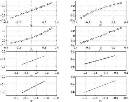
Figure 2: Output waveforms corresponding to the trellis shown in Fig. 1

Figure 3: Pruned trellis (Pruned edges are shown in dashed lines.)

Consider the root raised-cosine (RRC) pulse shaped QPSK modulation. The RRC shaping pulse is

$$\begin{split}p(t)=\frac{\sqrt{2W}}{(1-(8\alpha Wt)^{2})}\bigg{(}\frac{\sin(2\pi W(1-\alpha)t)}{2\pi Wt}\\ +\frac{4\alpha}{\pi}\cos(2\pi W(1+\alpha)t)\bigg{)},\end{split}$$ (2)

where $\alpha$ is the roll off factor and W is the ideal Nyquist bandwidth [2]. This paper considers a causal pulse shaping filter with finite length given by

$$\begin{split}\hat{p}(t)=\begin{cases}p(t-DT),\text{ if }0\leq t\leq 2DT\\ 0,\text{ otherwise}\end{cases},\end{split}$$ (3)

where $T$ is the symbol duration and the delay is $D$ symbols. Truncating length of the filter is equal to twice the delay. The filter output waveform is

$$s(t)=\sum_{i=0}^{\infty}g_{i}\hat{p}(t-iT),$$ (4)

where $\{g_{i}\}$ is the input sequence with symbols drawn from QPSK constellation.

We view the pulse shaping filter as a 4-ary convolutional encoder with $2D-1$ shift registers. Therefore, total number of states of the convolutional encoder is equal to $4^{2D-1}$. The output associated with the state transition initiated by the $j$th input QPSK message symbol $g_{j}$ is

$$s_{j} = s(t)$$ (5)

$$= \sum_{i=0}^{\infty}g_{i}\hat{p}(t-iT)$$ (6)

$$= \sum_{i=j-(2D-1)}^{j}g_{i}\hat{p}(t-iT)\text{, }$$ (7)

for $jT\leq t\leq(j+1)T$. From (7), $s_{j}$ is solely determined by the $j$th input and $2D-1$ message symbols stored in the shift register. An example of the trellis of such an encoder with 1024 states (D=3) is shown in Fig. 1. The corresponding output waveforms are listed in Fig. 2.

In (7), when $g_{i}\hat{p}(t-iT)$ adds constructively, the trajectory of $s_{j}$ goes far away from the origin; when $g_{i}\hat{p}(t-iT)$ adds destructively, the trajectory of $s_{j}$ goes close to the origin. Therefore, some edges of the trellis produce zero-crossing output waveforms (as is shown in Fig. 2 (a)-(d)), and some produce peaks (Fig. 2 (e)-(h)). Pruning such edges, i.e., eliminating the state transitions that generate large peak or zero-crossing, reduces the PAPR significantly. Take the trellis in Fig. 1 as example. Edge (d) and (h) will be pruned. The state transitions that follow the pruned edges will take one of the three remaining edges from the same state. The new trellis, which characterizes the pruning convolutional encoder, is shown in Fig. 3.

The trellis pruning method for QPSK modulation also applies to RRC filtered 16-QAM modulation. The only difference is that the pulse shaping filter is now viewed as a 16-ary convolutional encoder.

III PAPR Results

This section provides PAPR reduction results using the method described in Section II. There are many pruning strategies to choose from. This paper uses the following strategy: edges of the trellis that produce output waveforms going farthest away from the origin (peak) and passing nearest to the origin (zero-crossing) are simultaneously pruned. We use pruning percentage $\eta$ to measure how much pruning is actually performed. $\eta$ is defined as

$$\eta=\frac{\text{number of pruned edges}}{\text{total number of edges in the trellis}}.$$ (8)

All the filters used in the simulations have a delay $D$ of $3$ symbols. Fig. 4 shows the trajectory diagrams of RRC filtered QPSK signals without pruning and with $\eta=10\%$, $30\%$, $50\%$ pruning respectively. It is clear that with the increase of the pruning percentage, zero-crossing and peak waveforms are eliminated.

      

                       (a)                          (b)

      

                       (c)                          (d)

Figure 4: Trajectory diagrams of RRC filtered QPSK (a)w/o pruning, (b)$10\%$ pruning, (c)$30\%$ pruning, and (d)$50\%$ pruning.

The above pruning strategy is simulated for both QPSK and 16-QAM for various pruning percentage, where the shaping filters are the RRC filters of different roll-off factors. Fig. 5 and Fig. 6 shows that the pruning method can effectively reduce the PAPR of both modulation schemes. The reduction of the PAPR is more significant for 16-QAM: a $0.5\%$ pruning can reduce the PAPR by more than $25\%$.

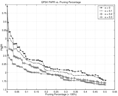
Figure 5: PAPR vs. pruning percentage for RRC filtered QPSK

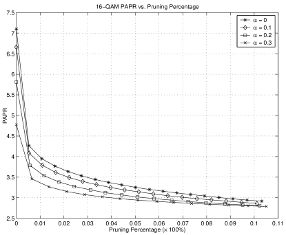
Figure 6: PAPR vs. pruning percentage for RRC filtered 16-QAM

IV Decoding Algorithm and Capacity

IV-A Decoding Algorithm

Viterbi algorithm is typically used to decode convolutional codes. However, the number of states of the encoder presented in this paper grows exponentially with the length of the pulse shaping filter and constellation size. With the increase of filter length and the expansion of constellation from QPSK to 16-QAM, the complexity of Viterbi algorithm makes it computationally intractable. Therefore, we use a forward only decision feedback aided BCJR algorithm with much lower complexity as the decoding algorithm.

\psfrag{x}{$\{X_{k}\}$}\psfrag{y}{$\{Y_{k}\}$}\includegraphics[width=216.81pt]{system_model.eps}

Figure 7: The pruning channel model

We model the pruning convolutional encoder as a finite-state machine (FSM) [11]. The concatenation of the FSM and the Additive White Gaussian Noise (AWGN) channel, as is shown in Fig. 7, is modelled as a Finite State Markov Channel (FSMC). We call this particular FSMC the pruning channel. The channel input process $\{X_{k}\}$ is assumed to be i.i.d. symbols drawn from a finite set $\mathcal{S}$. The state process $\{S_{k}\}$ forms an irreducible, aperiodic, stationary finite state Markov chain over a finite state space ${\mathcal{Q}}=\{1,\cdots,{K}\}$.The statistics of the FSMC satisfies the following properties:

• $P(X_{k}|S_{i})=P(X_{k})$ for $i\leq k$;

• Given $X_{k}$ and $S_{k}$, $\{Y_{k},S_{k+1}\}$ is statistically independent of $\{X_{i}\}_{i=1}^{k-1}$, $\{Y_{i}\}_{i=1}^{k-1}$, and $\{S_{i}\}_{i=1}^{k-1}$.

For FSMC, the standard BJCR [12] calculates the a posteriori probability (APP) of $X_{k}$ given past and future channel outputs $\{Y_{i}\}_{i=1}^{N}$. Whereas, the decision feedback aided BCJR (DFA-BCJR), proposed in [13] and [14], calculates the APP value of $X_{k}$ given a finite sequence of the past channel inputs $\{X_{i}\}_{i=1}^{k-1}$ and a finite sequence of past and future channel outputs $\{Y_{i}\}_{i=1}^{N}$. Denote $X_{1}^{k}\equiv\{X_{i}\}_{i=1}^{k}$ and $Y_{1}^{k}\equiv\{Y_{i}\}_{i=1}^{k}$ for notational convenience. From the Bayes rule,

$$P(X_{k}|Y_{1}^{N},X^{k-1}_{1})=\frac{P(Y_{1}^{N}|X^{k}_{1})P(X_{k})}{P(Y_{1}^{N}|X^{k-1}_{1})}.$$ (9)

We can rewrite the conditional probabilities as

$$P(Y_{1}^{N}|X^{k}_{1})=\sum_{s^{\prime}}\sum_{s}\alpha_{k}(s^{\prime})\gamma_{k+1}(s^{\prime},s,X_{k})\beta_{k+1}(s),$$ (10)

$$P(Y_{1}^{N}|X^{k-1}_{1})=\sum_{s^{\prime}}\sum_{s}\alpha_{k}(s^{\prime})\gamma_{k+1}(s^{\prime},s)\beta_{k+1}(s),$$ (11)

Where

$$\alpha_{k}(s^{\prime})=P(Y^{k-1}_{1},S_{k}=s^{\prime}|X_{1}^{k-1}),$$ (12)

$$\gamma_{k+1}(s^{\prime},s,X_{k})=P(Y_{k},S_{k+1}=s|S_{k}=s^{\prime},X_{k}),$$ (13)

$$\gamma_{k+1}(s^{\prime},s)=P(Y_{k},S_{k+1}=s|S_{k}=s^{\prime}),$$ (14)

$$\beta_{k+1}(s)=P(Y^{N}_{k+1}|S_{k+1}=s).$$ (15)

$\alpha_{k}$ denotes the forward path of the DFA-BCJR algorithm, while $\beta_{k}$ denotes the backward path. DFA-BCJR algorithm differs from the standard BCJR algorithm due to the presence of known input symbols in the forward path. Note that when given $X_{1}^{k-1}$, (12) can be rewritten as

$$\begin{split}\alpha_{k}(s^{\prime})=\begin{cases}1,\text{if }s^{\prime}\text{ takes on value determined by }X_{1}^{k-1}\\ 0,\text{otherwise}\end{cases}.\end{split}$$ (16)

Substitute (16) into (10) and (11),

$$P(Y_{1}^{N}|X^{k}_{1})=\sum_{s}\gamma_{k+1}(s^{\prime},s,X_{k})\beta_{k+1}(s),$$ (17)

$$P(Y_{1}^{N}|X^{k-1}_{1})=\sum_{s}\gamma_{k+1}(s^{\prime},s)\beta_{k+1}(s),$$ (18)

where the state $s^{\prime}$ takes on value determined by $X_{1}^{k-1}$.

Equation (17) and (18) show that with decision feedback, the complexity of the forward path calculation is independent of the number of states $K$ of the FSMC. However, the complexity of the backward path still grows exponentially with $K$. To further reduce complexity, we only use the forward path of the DFA-BCJR as the decoding algorithm. That is, when calculating the APP value of $X_{k}$, no future channel outputs $\{Y_{k}\}_{i=k+1}^{N}$ are available. Therefore, the APP value becomes

$$P(X_{k}|Y_{1}^{k},X^{k-1}_{1})=\frac{\sum_{s}\gamma_{k+1}(s^{\prime},s,X_{k})}{\sum_{s}\gamma_{k+1}(s^{\prime},s)}.$$ (19)

From (19), it is clear that the decoding algorithm has a complexity growing linearly with the number of states.

To achieve good performance of the decoding algorithm, we need to carefully choose the appropriate coding scheme before the convolutional encoder, such that accurate estimation of the previous input symbols can be obtained and then feedback to the decoding algorithm as known input symbols.

IV-B Capacity and Capacity Lower Bound

This section discusses how to calculate the capacity and capacity lower bound of the pruning channel. Simulation results show that pruning does not decrease capacity much. Here capacity refers to the constrained channel capacity of a given input distribution. We only consider $M$-ary i.i.d. inputs.

The capacity of the pruning channel, which is modelled as an FSMC shown in Fig. 7, is

$$C=\lim_{N\rightarrow\infty}\frac{1}{N}I({X_{1}^{N}};{Y_{1}^{N}}).$$ (20)

Expanding $\frac{1}{N}I(X^{N}_{1};Y^{N}_{1})$, we have

$$\frac{1}{N} I(X^{N}_{1};Y^{N}_{1})=\frac{1}{N}[H(X^{N}_{1})-H(X^{N}_{1}|Y^{N}_{1})]$$

$$=\log_{2}M-\frac{1}{N}\sum_{k=1}^{N}H(X_{k}|Y^{N}_{1},X_{1}^{k-1})$$ (21)

$$=\log_{2}M-\frac{1}{N}\sum_{k=1}^{N}E[-\log_{2}P(X_{k}|Y_{1}^{N},X_{1}^{k-1})].$$ (22)

As $N$ goes to infinity, (22) is the capacity of the pruning channel. $P(X_{k}|Y_{1}^{N},X_{1}^{k-1})$ in (22) can be computed by the DFA-BCJR algorithm. Therefore, we can calculate the channel capacity by Monte Carlo simulation of equation (9) to (18) and (22).

The computation becomes too complex when the filter length or $M$ is large. To simplify calculation, we derive a capacity lower bound as follows. Since conditioning reduces entropy, we have

$$H(X_{k}|Y^{N}_{1},X_{1}^{k-1})\leq H(X_{k}|Y_{1}^{k},X_{1}^{k-1}).$$ (23)

Substituting (23) into (21) yields

$$\frac{1}{N} I(X^{N}_{1};Y^{N}_{1})$$ (24)

$$\geq\log_{2}M-\frac{1}{N}\sum_{k=1}^{N}H(X_{k}|Y_{1}^{k},X_{1}^{k-1})$$ (25)

$$=\log_{2}M-\frac{1}{N}\sum_{k=1}^{N}E[-\log_{2}P(X_{k}|Y_{1}^{k},X_{1}^{k-1})].$$ (26)

Equation (26) is the capacity lower bound of the pruning channel. It can be simulated using equation (19). This lower bound is also the achievable rate of the forward only DFA-BCJR decoder discussed in Section IV-A.

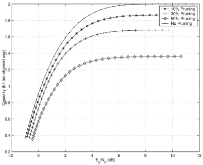
Figure 8: Capacity of the AWGN channel and the $10\%$, $30\%$, $50\%$ pruning channel with QPSK inputs

Figure 9: Capacity of the AWGN channel and capacity lower bound of the $1\%$, $4\%$, $7\%$ and $10\%$ pruning channel with 16-QAM inputs

Capacity of the pruning channel with QPSK inputs and capacity lower bound of the pruning channel with 16-QAM inputs are shown in Fig. 8 and Fig. 9 respectively. These results illustrate that, capacity loss, compared with the normal AWGN channel without pruning, is fairly small when pruning is less than $10\%$. For 16-QAM, $10\%$ pruning reduces the PAPR by more than a half. Define

$$\rho=\frac{\text{Capacity of the pruning channel}}{\text{Capacity of the normal AWGN channel}}$$ (27)

to represent the amount of capacity that is preserved after pruning. Fig. 10, which combines Fig. 6 and Fig. 9, further confirms that with a small loss of capacity, the pruning method can achieve significant PAPR reduction for filtered 16-QAM modulation.

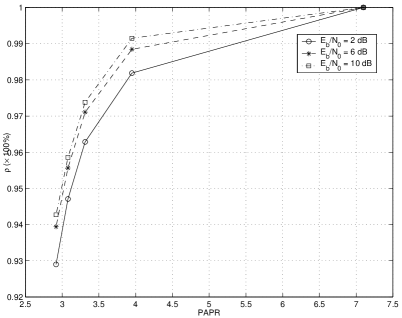
Figure 10: Percentage of capacity remaining after pruning vs. PAPR for RRC filtered 16-QAM signals

V Conclusion

This paper introduces a new trellis pruning method for reducing the PAPR of filtered QPSK and 16-QAM signals. The pulse shaping filter is viewed as a nonlinear convolutional encoder. Eliminating certain state transitions of the encoder can reduce the PAPR of transmitted signals. Simulation results confirm that this method can significantly reduce the PAPR of both QPSK and 16-QAM modulations.

Forward only DFA-BCJR algorithm is used as the decoding algorithm. DFA-BCJR algorithm also helps to calculate the capacity of the pruning channel. Capacity loss is small when pruning is less than $10\%$, which means for 16-QAM, reducing the PAPR by more than a half only costs a negligible capacity loss.

References

- [1] H. Ochiai and H. Imai, “Performance analysis of deliberately clipped OFDM signals,” IEEE Trans. on Communications, vol. 50, no. 1, pp. 89 – 101, January 2002.
- [2] S. Haykin and M. Moher, Modern Wireless Communications, Prentice Hall, 2004.
- [3] S. Haykin, Communications Systems, Wiley, 4th edition, 2000.
- [4] Cheng-Po Liang, Je-Hong Jong, W.E. Stark, and J.R. East, “Nonlinear amplifier effects in communications systems,” IEEE Transactions on Microwave Theory and Techniques, vol. 47, no. 8, pp. 1461 – 1466, August 1999.
- [5] K. Murota and K. Hirade, “GMSK modulation for digital mobile radio telephony,” IEEE Trans. on Communications, vol. 29, no. 7, pp. 1044 – 1050, July 1981.
- [6] T. Aulin, N. Rydbeck, and C.-E. Sundberg, “Continuous Phase Modulation–Part II: Partial Response Signaling,” IEEE Trans. on Communications, vol. 29, no. 3, pp. 210 – 225, March 1981.
- [7] S. Kato and K. Feher, “XPSK: A new cross-correlated phase-shift keying modulation technique,” IEEE Trans. on Communications, vol. 31, no. 5, pp. 701 – 707, May 1983.
- [8] Hyo-Joo Ahn, Yoan Shin, and Sungbin Im, “A block coding scheme for peak-to-average power ratio reduction in an orthogonal frequency division multiplexing system,” in Proc. Veh. Tech. Conf. (VTC 2000-Spring), Tokyo, Japan, May 2000, vol. 1, pp. 56 – 60.
- [9] Pingyi Fan and Xiang-Gen Xia, “Block coded modulation for the reduction of the peak to average power ratio in OFDM systems,” in Wireless Communications and Networking Conference (WCNC ’99), 1999, pp. 1095 – 1099.
- [10] T.A. Wilkinson and A.E. Jones, “Minimisation of the peak to mean envelope power ratio of multicarrier transmission schemes by block coding,” in Proc. Veh. Tech. Conf. (VTC ’95), 1995, pp. 825 – 829.
- [11] S. Lin and D. J. Costello Jr., Error Control Coding, Prentice Hall, 2nd edition, 2004.
- [12] L. Bahl, J. Cocke, F. Jelinek, and J. Raviv, “Optimal decoding of linear codes for minimizing symbol error rate,” IEEE Trans. on Information Theory, vol. 20, no. 2, pp. 284–287, March 1974.
- [13] O. M. Collins, “Coding for the variably coherent channel,” in Proc. IEEE International symposium on Information Theory, Chicago, USA, June 2004.
- [14] Teng Li and O. M. Collins, “A successive decoding strategy for channels with memory,” in Proc. IEEE International symposium on Information Theory, Adelaide, Australia, September 2005.