Verifying nondeterministic probabilistic channel systems against $\omega$-regular linear-time properties

Abstract

Lossy channel systems (LCS’s) are systems of finite state processes that communicate via unreliable unbounded fifo channels. We introduce NPLCS’s, a variant of LCS’s where message losses have a probabilistic behavior while the component processes behave nondeterministically, and study the decidability of qualitative verification problems for $\omega$-regular linear-time properties.

We show that – in contrast to finite-state Markov decision processes – the satisfaction relation for linear-time formulas depends on the type of schedulers that resolve the nondeterminism. While the qualitative model checking problems for the full class of history-dependent schedulers is undecidable, the same questions for finite-memory schedulers can be solved algorithmically. Additionally, some special kinds of reachability, or recurrent reachability, qualitative properties yield decidable verification problems for the full class of schedulers, which – for this restricted class of problems – are as powerful as finite-memory schedulers, or even a subclass of them.

Authors’ adresses: C. Baier, Universität Bonn, Institut für Informatik, Römerstr. 164, D-53117 Bonn, Germany.
N. Bertrand and Ph. Schnoebelen, Laboratoire Spécification et Vérification, ENS de Cachan, 61 av. Pdt Wilson, 94235 Cachan Cedex, France.
This research was supported by Persée, a project of the ACI Sécurité Informatique, by PROBPOR, a DFG-project, and by VOSS, a DFG-NWO-project.

1 Introduction

Channel systems [Brand and Zafiropulo (1983)] are systems of finite-state components that communicate via asynchronous unbounded fifo channels. See Fig. 1 for an example of a channel systems with two components $E_{1}$ and $E_{2}$ that communicate through fifo channels $c_{1}$ and $c_{2}$. Lossy channel systems [Finkel (1994), Abdulla and Jonsson (1996b)] are a special class of channel systems where messages can be lost while they are in transit, without any notification. Considering lossy systems is natural when modeling fault-tolerant protocols where the communication channels are not supposed to be reliable. Additionally, the lossiness assumption makes termination and safety properties decidable [Pachl (1987), Finkel (1994), Cécé et al. (1996), Abdulla and Jonsson (1996b)].

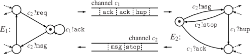
Figure 1: A channel system: $E_{1}$ and $E_{2}$ communicate through channels $c_{1}$ and $c_{2}$.

Several important verification problems are undecidable for these systems, including recurrent reachability, liveness properties, boundedness, and all behavioral equivalences [Abdulla and Jonsson (1996a), Schnoebelen (2001), Mayr (2003)]. Furthermore, the above-mentioned decidable problems cannot be solved in primitive-recursive time [Schnoebelen (2002)].

Verifying Liveness Properties

Lossy channel systems are a convenient model for verifying safety properties of asynchronous protocols, and such verifications can sometimes be performed automatically [Abdulla et al. (2004)]. However, they are not so adequate for verifying liveness properties. A first difficulty here is the undecidability of liveness properties.

A second difficulty is that the model itself is too pessimistic when liveness is considered. Protocols that have to deal with unreliable channels usually have some coping mechanisms combining resends and acknowledgments. But, without any assumption limiting message losses, no such mechanism can ensure that some communication will eventually be initiated. The classical solution to this problem is to add some fairness assumptions on the channel message losses, e.g., “if infinitely many messages are sent through the channels, infinitely many of them will not be lost”. However, fairness assumptions in lossy channel systems make decidability more elusive [Abdulla and Jonsson (1996a), Masson and Schnoebelen (2002)].

Probabilistic Losses

When modeling protocols, it is natural to see message losses as some kind of faults having a probabilistic behavior. Following this idea, Purushothaman Iyer and Narasimha purush97 introduced the first Markov chain model for lossy channel systems, where message losses (and other choices) are probabilistic. In this model, verification of qualitative properties is decidable when message losses have a high probability [Baier and Engelen (1999)] and undecidable otherwise [Abdulla et al. (2005)]. An improved model was later introduced by ABRS-icomp where the probability of losses is modeled more faithfully and where qualitative verification (and approximate quantitative verification [Rabinovich (2003)]) is decidable independently of the likelihood of message losses. See the survey by Sch-voss for more details.

These models are rather successful in bringing back decidability. However, they assume that the system is fully probabilistic, i.e., the choice between different actions is made probabilistically. But when modeling channel systems, nondeterminism is an essential feature. It is used to model the interleaved behavior of distributed components, to model an unknown environment, to delay implementation choices at early stages of the design, and to abstract away from complex control structures at later stages.

Our Contribution

We introduce Nondeterministic Probabilistic Lossy Channel Systems (NPLCS), a new model where channel systems behave nondeterministically while messages are lost probabilistically, and for which the operational semantics is given via infinite-state Markov decision processes. For these NPLCS’s, we study the decidability of qualitative $\omega$-regular linear-time properties. We focus here on “control-based” properties, i.e., temporal formulas where the control locations of the given NPLCS serve as atomic propositions.

There are eight variants of the qualitative verification problem for a given $\omega$-regular property $\varphi$ and a starting configuration $s$, that arise from

• the four types of whether $\varphi$ should hold almost surely (that is, with probability 1), with positive probability, with zero probability or with probability less than 1

• existential or universal quantification over all schedulers, i.e., instances that resolve the nondeterministic choices.

By duality of existential and universal quantification, it suffices to consider the four types of probabilistic satisfaction and one variant of quantification (existential or universal). We deal with the case of existential quantification since it is technically more convenient.

Our main results can be summarized as follows. First, we present algorithms for reachability properties stating that a certain set of locations will eventually be visited. We then discuss repeated reachability properties. While repeated reachability problems with the three probabilistic satisfaction relations “almost surely”, “with zero probability” and “with probability less than 1” can be solved algorithmically, the question whether a certain set of locations can be visited infinitely often “with positive probability” under some scheduler is undecidable. It appears that this is because schedulers are very powerful (e.g., they need not be recursive). In order to recover decidability without sacrificing too much of the model, we advocate restricting oneself to finite-memory schedulers, and show this restriction makes the qualitative model checking problem against $\omega$-regular properties decidable for NPLCS’s.

This article is partly based on, and extends, material presented in [Bertrand and Schnoebelen (2003), Bertrand and Schnoebelen (2004)]. However, an important difference with this earlier work is that the NPLCS model we use does not require the presence of idling steps (see Remark 2.3 below). This explains why some of the results presented here differ from those in [Bertrand and Schnoebelen (2003), Bertrand and Schnoebelen (2004)].

Outline of the Article

Section 2 introduces probabilistic lossy channel systems and their operational semantics. Section 3 establishes some fundamentals properties, leading to algorithms for reachability and repeated reachability problems (in section 4). Section 5 shows that some repeated reachability problems are undecidable and contains other lower-bound results. Section 6 shows decidability for problems where attention is restricted to finite-memory schedulers, and section 7 shows how positive results for Streett properties generalize to arbitrary $\omega$-regular properties. Finally, section 8 concludes the article.

2 Nondeterministic probabilistic channel systems

Lossy channel systems

A lossy channel system (a LCS) is a tuple ${\mathcal{L}}=(Q,{\mathsf{C}},{\mathsf{M}},\Delta)$ consisting of a finite set $Q=\{p,q,\ldots\}$ of control locations (also called control states), a finite set ${\mathsf{C}}=\{c,\ldots\}$ of channels, a finite message alphabet ${\mathsf{M}}=\{m,\ldots\}$ and a finite set $\Delta=\{\delta,\ldots\}$ of transition rules. Each transition rule has the form $q\xrightarrow{\!\!{\mathit{op}}\!\!}p$ where ${\mathit{op}}$ is an operation of the form

• ${c}!m$ (sending message $m$ along channel ${c}$),

• ${c}?m$ (receiving message $m$ from channel ${c}$),

• $\surd$ (an internal action to some process, no I/O-operation).

The control graph of ${\mathcal{L}}$ is the directed graph having the locations of ${\mathcal{L}}$ as its nodes and rules from $\Delta$ for its edges. It is denoted with ${\mathit{Graph}}(Q)$, and more generally ${\mathit{Graph}}(A)$ for $A\subseteq Q$ denote the control graph restricted to locations in $A$.

Our introductory example in Fig. 1 is turned into a LCS by replacing the two finite-state communicating agents $E_{1}$ and $E_{2}$ by the single control automaton one obtains with the asynchronous product $E_{1}\times E_{2}$.

Operational Semantics. Let ${\mathcal{L}}=(Q,{\mathsf{C}},{\mathsf{M}},\Delta)$ be a LCS. A configuration, also called global state, is a pair $(q,w)$ where $q\in Q$ is a location and $w:{\mathsf{C}}\to{\mathsf{M}}^{*}$ is a channel valuation that associates with any channel its content (a sequence of messages). We write ${{\mathsf{M}}^{*}}^{\mathsf{C}}$ for the set of all channel valuations, or just ${\mathsf{M}}^{*}$ when $|{\mathsf{C}}|=1$. The set $Q\times{{\mathsf{M}}^{*}}^{\mathsf{C}}$ of all configurations is denoted by ${\mathsf{Conf}}$. With abuse of notations, we shall use the symbol $\varepsilon$ for both the empty word and the channel valuation where all channels are empty. If $s=(q,w)$ is a configuration then we write $|s|$ for the total number of messages in $s$, i.e., $|s|=|w|=\sum_{{c}\in{\mathsf{C}}}|w({c})|$.

We say that a transition rule $\delta=q\xrightarrow{\!\!{\mathit{op}}\!\!}p$ is enabled in configuration $s=(r,w)$ iff

1. the current location is $q$, i.e., $r=q$, and

2. performing ${\mathit{op}}$ is possible. This may depend on the channels contents: sending and internal actions are always enabled, while a receiving ${c}?m$ is only possible if the current content of channel ${c}$ starts with the message $m$, i.e., if the word $w({c})$ belongs to $m{\mathsf{M}}^{*}$.

For $s$ a configuration, we write $\Delta(s)$ for the set of transition rules that are enabled in $s$.

When $\delta=p\xrightarrow{\!\!{\mathit{op}}\!\!}q$ is enabled in $s=(q,w)$, firing $\delta$ yields a configuration $s^{\prime}=(p,{\mathit{op}}(w))$ where ${\mathit{op}}(w)$ denotes the new contents after executing ${\mathit{op}}$:

• if ${\mathit{op}}=\surd$, then ${\mathit{op}}(w)=w$,

• if ${\mathit{op}}={c}!m$, then ${\mathit{op}}(w)({c})=w({c})m$, and ${\mathit{op}}(w)({c}^{\prime})=w({c}^{\prime})$ for ${c}\neq{c}^{\prime}$,

• if ${\mathit{op}}={c}?m$ (and then $w({c})$ is some $m\mu$ since $\delta$ was enabled), then ${\mathit{op}}(w)({c})=\mu$, and ${\mathit{op}}(w)({c}^{\prime})=w({c}^{\prime})$ for ${c}\neq{c}^{\prime}$.

We write $s\xrightarrow{\!\!\delta\!\!}_{\textrm{perf}}s^{\prime}$ when $s^{\prime}$ is obtained by firing $\delta$ in $s$. The “perf” subscript stresses that the step is perfect: no messages are lost.

However, in lossy systems, arbitrary messages can be lost. This is formalized with the help of the subword ordering: we write $\mu\sqsubseteq\mu^{\prime}$ when $\mu$ is a subword of $\mu^{\prime}$, i.e., $\mu$ can be obtained by removing any number of messages from $\mu^{\prime}$, and we extend this to configurations, writing $(q,w)\sqsubseteq(q^{\prime},w^{\prime})$ when $q=q^{\prime}$ and $w({c})\sqsubseteq w^{\prime}({c})$ for all $c\in{\mathsf{C}}$. By Higman’s Lemma, $\sqsubseteq$ is a well-quasi-order between configurations of ${\mathcal{L}}$ [Abdulla et al. (2000), Finkel and Schnoebelen (2001)].

Now, we define lossy steps by letting $s\xrightarrow{\!\!\delta\!\!}s^{\prime\prime}$ whenever there is a perfect step $s\xrightarrow{\!\!\delta\!\!}_{\textrm{perf}}s^{\prime}$ such that $s^{\prime\prime}\sqsubseteq s^{\prime}$. This gives rise to a labeled transition system ${\mathit{LTS}}_{\mathcal{L}}\stackrel{{\scriptstyle\mbox{\scriptsize def}}}{{=}}({\mathsf{Conf}},\Delta,\to)$. Here the set $\Delta$ of transition rules serves as action alphabet.

Remark 2.1.

In the following we only consider LCS’s where, for any location $q\in Q$, $\Delta$ contains at least one rule $q\xrightarrow{\!\!{\mathit{op}}\!\!}p$ where ${\mathit{op}}$ is not a receive operation. This ensures that ${\mathit{LTS}}_{\mathcal{L}}$ has no terminal configuration, where no rules are enabled. ∎

Notation 2.2 ((Arrow-notations)).

Let $s$, $t\in{\mathsf{Conf}}$ be configurations. We write $s\to t$ if $s\xrightarrow{\!\!\delta\!\!}t$ for some $\delta$. As usual, $\xrightarrow{\!\!+\!\!}$ (resp. $\xrightarrow{\!\!*\!\!}$) denotes the transitive (resp.  reflexive and transitive) closure of $\to$. Let $\leadsto$ be $\to$, $\xrightarrow{\!\!*\!\!}$ or $\xrightarrow{\!\!+\!\!}$. For $T\subseteq{\mathsf{Conf}}$, we write $s\leadsto T$ when $s\leadsto t$ for some $t\in T$. When $X\subseteq Q$ is a set of locations $s\leadsto X$ means that $s\leadsto(x,w)$ for some $x\in X$ (and for some $w$).

We also use a special notation for constrained reachability: $s\xrightarrow{\!\!*\!\!}_{[X]}t$ means that there is a sequence of steps going from configuration $s$ to $t$ and visiting only locations from $X$, including at the two extremities $s$ and $t$. With $s\xrightarrow{\!\!*\!\!}_{[X)}t$ we mean that the constraint does not apply to the last configuration. Hence $s\xrightarrow{\!\!*\!\!}_{[X)}s$ is always true, even with empty $X$. The following equivalence links the two notions:

$$s\xrightarrow{\!\!*\!\!}_{[X)}t\;\;\text{iff}\;\;\Bigl{[}s=t\;\text{ or }\;\exists s^{\prime}\bigl{(}s\xrightarrow{\!\!*\!\!}_{[X]}s^{\prime}\text{ and }s^{\prime}\xrightarrow{\!\!\!\!}t\bigr{)}\Bigr{]}.\qed$$

We recall that in LCS’s the following constrained reachability questions: “given $s,t$ configurations, $X\subseteq Q$ and $\leadsto\in\{\to,\xrightarrow{\!\!*\!\!},\xrightarrow{\!\!+\!\!}\}$ does $s\leadsto_{[X]}t$ (or $s\leadsto_{[X)}t$)?” are decidable [Abdulla and Jonsson (1996b), Schnoebelen (2002)].

The MDP-semantics

Following Bertrand and Schnoebelen BS03,BS04, we define the operational behavior of a LCS by an infinite-state Markov decision process. A NPLCS ${\mathcal{N}}=({\mathcal{L}},\tau)$ consists of a LCS ${\mathcal{L}}$ and a fault rate $\tau\in(0,1)$ that specifies the probability that a given message stored in one of the message queues is lost during a step. In the sequel, for $w,w^{\prime}\in{{\mathsf{M}}^{*}}^{\mathsf{C}}$, we let ${\textbf{P}}_{\mathit{lost}}(w,w^{\prime})$ denote the probability that channels containing $w$ change to $w^{\prime}$ within a single step as a result of message losses. This requires losing $|w|-|w^{\prime}|$ message at the right places. Formally, we let

$${\textbf{P}}_{\mathit{lost}}(w,w^{\prime})\stackrel{{\scriptstyle\mbox{\scriptsize def}}}{{=}}\tau^{|w|-|w^{\prime}|}\cdot(1-\tau)^{|w^{\prime}|}\cdot\binom{w}{w^{\prime}}$$ (1)

where the combinatorial coefficient $\binom{w}{w^{\prime}}$, is the number of different embeddings of $w^{\prime}$ in $w$. For instance, in the case where $w=aaba$, one has

$\binom{aaba}{a}=\binom{aaba}{aa}=3$,   $\binom{aaba}{aba}=\binom{aaba}{ab}=2$,   $\binom{aaba}{w^{\prime}}=1\text{ \ if \ }w^{\prime}\in\{\varepsilon,b,aaa,aab,ba,aaba\}$

and $\binom{aaba}{w^{\prime}}=0$ in all other cases. Note that, e.g., $w^{\prime}=aa$ can be obtained from $w=aaba$ in three different ways (by removing the $b$ and either the first, second or third $a$), while $w^{\prime}=ba$ is obtained from $w$ in a unique way (by removing the first two $a$’s). See [Abdulla et al. (2005)] for more details. Here, it is enough to know that $\binom{w}{w^{\prime}}\neq 0\text{ iff }w^{\prime}\sqsubseteq w$ and that the probabilities add up to one: for all $w$, $\sum_{w^{\prime}}{\textbf{P}}_{\mathit{lost}}(w,w^{\prime})=1$.

The Markov decision process associated with ${\mathcal{N}}$ is ${\mathit{MDP}}_{\mathcal{N}}\stackrel{{\scriptstyle\mbox{\scriptsize def}}}{{=}}({\mathsf{Conf}},\Delta,{\textbf{P}}_{\mathcal{N}})$. The stepwise probabilistic behavior is formalized by a three-dimensional transition probability matrix ${\textbf{P}}_{\mathcal{N}}:{\mathsf{Conf}}\times\Delta\times{\mathsf{Conf}}\to[0,1]$. For a given configuration $s$ and a transition rule $\delta$ that is enabled in $s$, ${\textbf{P}}_{\mathcal{N}}(s,\delta,\cdot)$ is a distribution over the states in ${\mathit{MDP}}_{\mathcal{N}}$, while ${\textbf{P}}_{\mathcal{N}}(s,\delta,\cdot)=0$ for any transition rule $\delta$ that is not enabled in $s$. The intuitive meaning of ${\textbf{P}}_{\mathcal{N}}(s,\delta,t)=\lambda\mathchar 8510\relax 0$ is that with probability $\lambda$, the system moves from configuration $s$ to configuration $t$ when $\delta$ is the chosen transition rule in $s$. Formally, if $s=(q,w)$, $t=(p,w^{\prime})$, and $\delta=q\xrightarrow{\!\!{\mathit{op}}\!\!}p$ is enabled in $s$, then

$${\textbf{P}}_{\mathcal{N}}(s,\delta,t)\stackrel{{\scriptstyle\mbox{\scriptsize def}}}{{=}}{\textbf{P}}_{\mathit{lost}}({\mathit{op}}(w),w^{\prime}).$$ (2)

See Fig. 2 for an example where $s=(q,ab)$ and $\delta=q\xrightarrow{\!\!!b\!\!}p$.

Figure 2: From a LCS ${\mathcal{L}}$ to $MPD_{\mathcal{L}}$

A consequence of (1) and (2) is that the labeled transition system underlying ${\mathit{MDP}}_{\mathcal{L}}$ is exactly ${\mathit{LTS}}_{\mathcal{L}}$. Hence any path in ${\mathit{MDP}}_{\mathcal{L}}$ is also a path in ${\mathit{LTS}}_{\mathcal{L}}$ and the fact that ${\mathit{LTS}}_{\mathcal{L}}$ had no terminal configuration implies that there is no terminal state in ${\mathit{MDP}}_{\mathcal{L}}$.

Remark 2.3 ((The idling MDP semantics)).

The above definition of the MDP semantics for an NPLCS differs from the approach of Bertrand and Schnoebelen BS03,BS04 where each location $q$ is assumed to be equipped with an implicit idling transition rule $q\xrightarrow{\!\!\surd\!\!}q$. This idling MDP semantics allows simplifications in algorithms, but it does not respect enough the intended liveness of channel systems (e.g., inevitability becomes trivial) and we do not adopt it here. Observe that the new approach is more general since idling rules are allowed at any location in ${\mathcal{L}}$. ∎

Schedulers (finite-memory, memoryless, blind and almost blind)

Before one may speak of the probabilities of certain events in an MDP, the nondeterminism has to be resolved by means of a scheduler, also often called adversary, policy or strategy. We will use the word “scheduler” for a history-dependent deterministic scheduler in the classification of Puterman94. Formally, a scheduler for ${\mathcal{N}}$ is a mapping ${\mathcal{U}}$ that assigns to any finite path $\pi$ in ${\mathcal{N}}$ a transition rule $\delta\in\Delta$ that is enabled in the last state of $\pi$. Intuitively, the given path $\pi$ specifies the history of the system, and ${\mathcal{U}}(\pi)$ is the rule that ${\mathcal{U}}$ chooses to fire next.

A scheduler ${\mathcal{U}}$ only gives rise to certain paths in the MDP: we say $\pi=s_{1}\to s_{2}\to\cdots$ is compatible with ${\mathcal{U}}$ or, shortly, is a ${\mathcal{U}}$-path, if ${\textbf{P}}_{\mathcal{N}}(s_{n},\delta_{n},s_{n+1})\mathchar 8510\relax 0$ for all $n\geq 1$, where $\delta_{n}={\mathcal{U}}(s_{1}\to\cdots\to s_{n})$ is the transition rule chosen by ${\mathcal{U}}$ for the $n$-th prefix of $\pi$. In practice, it is only relevant to define how ${\mathcal{U}}$ evaluates on ${\mathcal{U}}$-paths.

In general ${\mathcal{U}}$ can be any function and, e.g., it needs not be recursive. It is often useful to consider restricted types of schedulers. In this article, the two main types of restricted schedulers we use are finite-memory schedulers, that abstract the whole history into some finite-state information, and blind schedulers, that ignore the contents of the channels.

Formally, a finite-memory scheduler for ${\mathcal{N}}$ is a tuple ${\mathcal{U}}=(U,D,\eta,u_{0})$ where $U$ is a finite set of modes, $u_{0}\in U$ is the starting mode, $D:U\times{\mathsf{Conf}}\to\Delta$ is the decision rule which assigns to any pair $(u,s)$ consisting of a mode $u\in U$ and a configuration $s$ a transition rule $\delta\in\Delta(s)$, and $\eta:U\times{\mathsf{Conf}}\to U$ is a next-mode function which describes the mode-changes of the scheduler. The modes can be used to store some relevant information about the history. In a natural way, a finite-memory scheduler can be viewed as a scheduler in the general sense: given a finite path $\pi=s_{0}\to s_{1}\to\cdots\to s_{n}$ in ${\mathcal{N}}$, it chooses $D(u,s_{n})$ where $u=\eta(u_{0},s_{0}s_{1}\ldots s_{n})=\eta(\ldots\eta(\eta(u_{0},s_{0}),s_{1}),\ldots,s_{n})$.

A scheduler ${\mathcal{U}}$ is called memoryless if ${\mathcal{U}}$ is finite-memory with a single mode. Thus, memoryless schedulers make the same decision for all paths that end up in the same configuration. In this sense, they are not history-dependent and can be defined more simply via mappings ${\mathcal{U}}:{\mathsf{Conf}}\to\Delta$.

By a blind scheduler, we mean a scheduler where the decisions only depend on the locations that have been passed, and not on the channel contents. Hence a blind scheduler never selects a reading transition rule. Observe that, since the probabilistic choices only affect channel contents (by message losses), all ${\mathcal{U}}$-paths generated by a blind ${\mathcal{U}}$ visit the same locations in the same order. More formally, with any initial locations $q_{0}$, a blind scheduler can be seen as associating an infinite sequence $q_{0}\xrightarrow{\!\!{\mathit{op}}_{1}\!\!}q_{1}\xrightarrow{\!\!{\mathit{op}}_{2}\!\!}q_{2}\cdots$ of chained transition rules and the ${\mathcal{U}}$-paths are exactly the paths of the form $(q_{0},w_{0})\to(q_{1},w_{1})\to(q_{2},w_{2})\to\cdots$ with $w_{i}\sqsubseteq{\mathit{op}}_{i}(w_{i-1})$ for all $i>0$.

A scheduler is called almost blind if it almost surely eventually behaves blindly. Formally, ${\mathcal{U}}$ is almost blind iff there exists a scheduler ${\mathcal{W}}$ and a blind scheduler ${\mathcal{V}}$ such that for all configurations $s$ and for almost all (see below) infinite ${\mathcal{U}}$-paths $\pi=s_{1}\to s_{2}\to\cdots$ with $s=s_{1}$, there exists an index $n\geq 0$ such that

• ${\mathcal{U}}(s_{1}\to\cdots\to s_{i})={\mathcal{W}}(s_{1}\to\cdots\to s_{i})$ for all indices $i\leq n$ and

• ${\mathcal{U}}(s_{1}\to\cdots\to s_{i})={\mathcal{V}}(s_{1}\to\cdots\to s_{i})$   for all indices $i\mathchar 8510\relax n$.

Here and in the sequel, the formulation “almost all paths have property $x$” means that the paths where property $x$ is violated are contained in some measurable set of paths that has probability measure 0. The underlying probability space is the standard one (briefly explained below).

Stochastic process

Given an NPLCS ${\mathcal{N}}$ and a scheduler ${\mathcal{U}}$, the behavior of ${\mathcal{N}}$ under ${\mathcal{U}}$ can be formalized by an infinite-state Markov chain ${\mathit{MC}}_{\mathcal{U}}$. For arbitrary schedulers, the states of ${\mathit{MC}}_{\mathcal{U}}$ are finite paths in ${\mathcal{N}}$. Intuitively, such a finite path $\pi=s_{1}\to\cdots\to s_{n-1}\to s_{n}$ represents configuration $s_{n}$, while $s_{1}\to\cdots\to s_{n-1}$ stand for the history how configuration $s_{n}$ was reached. If $\pi$ is a finite path ending in configuration $s$, and $\pi^{\prime}=\pi\to t$ is $\pi$ followed by step $s\to t$, then the probability ${\textbf{P}}_{\mathcal{U}}(\pi,\pi^{\prime})$ in ${\mathit{MC}}_{\mathcal{U}}$ is defined with ${\textbf{P}}_{\mathcal{U}}(\pi,\pi^{\prime})\stackrel{{\scriptstyle\mbox{\scriptsize def}}}{{=}}{\textbf{P}}_{\mathcal{N}}(s,{\mathcal{U}}(\pi),t)$, according to the chosen rule ${\mathcal{U}}(\pi)$. In all other cases ${\textbf{P}}_{\mathcal{U}}(\pi,\pi^{\prime})=0$. We now may apply the standard machinery for Markov chains and define (for fixed starting configuration $s$) a sigma-field on the set of infinite paths starting in $s$ and a probability measure on it, see, e.g., [Kemeny et al. (1966), Puterman (1994), Panangaden (2001)]. We shall write $\Pr_{\mathcal{U}}\bigl{(}s\models\cdots\bigr{)}$ to denote the standard probability measure in ${\mathit{MC}}_{\mathcal{U}}$ with starting state $s$.

For ${\mathcal{U}}$ a finite-memory scheduler, we can think of the states in ${\mathit{MC}}_{\mathcal{U}}$ as pairs $(u,s)$ consisting of a mode $u$ and a configuration $s$. In the sequel, we will write $s_{u}$ rather than $(u,s)$ as the intuitive meaning of $(u,s)$ is “configuration $s$ in mode $u$”. For finite-memory schedulers the successor-states of $s_{u}$ and their probabilities in ${\mathit{MC}}_{\mathcal{U}}$ are given by the MDP for ${\mathcal{N}}$ in configuration $s$ and the chosen transition rule for $s_{u}$. That is, if ${\mathcal{U}}$ is some $(U,D,\eta,u_{0})$, we have ${\textbf{P}}_{\mathcal{U}}(s_{u},t_{\eta(u,s)})\stackrel{{\scriptstyle\mbox{\scriptsize def}}}{{=}}{\textbf{P}}_{\mathcal{N}}(s,D(u,s),t)$, and if $u^{\prime}\neq\eta(u,s)$ then ${\textbf{P}}_{\mathcal{U}}(s_{u},t_{u^{\prime}})=0$. In a similar way, we can think of the Markov chains for memoryless or blind schedulers in a simpler way. For memoryless schedulers, the configurations of ${\mathcal{N}}$ can be viewed as states in the Markov chain ${\mathit{MC}}_{\mathcal{U}}$, while for blind schedulers we may deal with finite words over $Q$ complemented with some current channel contents.

LTL-notation

Throughout the article, we assume familiarity with linear temporal logic (LTL), see, e.g., [Emerson (1990)]. We use simple LTL formulas to denote properties of paths in ${\mathit{MDP}}_{\mathcal{L}}$. Here configurations and locations serve as atomic propositions: for example $\Box\Diamond s$ (resp. $\Box\Diamond x$) means that $s\in{\mathsf{Conf}}$ (resp. $x\in Q$) is visited infinitely many times along a path, and $x\mathrel{\mathit{Until}}s$ means that the control state remains $x$ until $s$ is eventually reached. These notations extend to sets: $\Box\Diamond T$ and $\Box\Diamond A$ for $T\subseteq{\mathsf{Conf}}$ and $A\subseteq Q$ with obvious meanings. For $A\subseteq Q$, $A_{\varepsilon}$ is the set $\{(q,\varepsilon):q\in A\}$ so that $\Diamond Q_{\varepsilon}$ means that eventually a configuration with empty channels is reached. It is well-known that for any scheduler ${\mathcal{U}}$, the set of paths starting in some configuration $s$ and satisfying an LTL formula, or an $\omega$-regular property, $\varphi$ is measurable [Vardi (1985), Courcoubetis and Yannakakis (1995)]. We write $\Pr_{\mathcal{U}}\bigl{(}s\models\varphi\bigr{)}$ for this measure.

Finite attractor

The crucial point for the algorithmic analysis of NPLCS is the fact that almost surely, a configuration where all channels are empty will be visited infinitely often. If ${\mathcal{U}}$ is a scheduler and $T$ a set of configurations then $T$ is called an attractor for ${\mathcal{U}}$ iff $\Pr_{\mathcal{U}}\bigl{(}s\models\Box\Diamond T\bigr{)}=1$ for any starting configuration $s$.

Proposition 2.4 ((Finite-attractor property for arbitrary schedulers))

For any scheduler ${\mathcal{U}}$, the set $Q_{\varepsilon}=\{(q,\varepsilon):q\in Q\}$ is a finite attractor for ${\mathcal{U}}$.

That is, almost all paths in ${\mathit{MC}}_{\mathcal{U}}$ visit $Q_{\varepsilon}$ infinitely often, independent on the starting state. We refer to [Bertrand and Schnoebelen (2003), Baier et al. (2006)] for formal proofs. An intuitive explanation of the result is that when the channels contain $n$ messages, each step can only add at most one new message (through a sending action) while on average $n\times\tau$ are lost. Thus when $n$ is large, it tends to decrease and this suffices to ensure that almost surely all messages will be lost.

3 Safe sets and Promising sets

At many places, our arguments use the notion of “safe sets” and “promising sets” of locations. In this section we define these notions, relate them to behavioral features, and explain how to compute them.

3.1 Safe sets

Definition 3.1.

Let ${\mathcal{L}}=(Q,{\mathsf{C}},{\mathsf{M}},\Delta)$ be a lossy channel system and $A\subseteq Q$ be a set of locations. We say that $X\subseteq Q$ is safe for $A$ if $X\subseteq A$ and $(x,\varepsilon)\to X$ for all $x\in X$.

Assume $A\subseteq Q$. It is easy to see that if $X$ and $Y$ are both safe for $A$, then $X\cup Y$ is safe for $A$ too. The same holds for infinite unions. As a consequence, the largest safe set for $A$ exists (union of all safe sets); it is denoted by ${\mathit{Safe}}(A)$, or ${\mathit{Safe}}$ when there is no ambiguity on $A$.

Observe that for any family $(A_{i})_{i\in I}$ of sets of locations, one has the following inclusions

$${\mathit{Safe}}\Bigl{(}\bigcup_{i\in I}A_{i}\Bigr{)}\>\supseteq\>\bigcup_{i\in I}{\mathit{Safe}}(A_{i}) \qquad{\mathit{Safe}}\Bigl{(}\bigcap_{i\in I}A_{i}\Bigr{)}\>\subseteq\>\bigcap_{i\in I}{\mathit{Safe}}(A_{i})$$ (3)

while the reverse inclusions do not hold in general.

${\mathit{Safe}}(A)$ can be computed in linear time: consider ${\mathit{Graph}}(A)$ the control graph restricted to locations of $A$. Remove from ${\mathit{Graph}}(A)$ the edges that carry receiving operations “${c}?m$”. The nodes that have no outgoing edges cannot be in ${\mathit{Safe}}(A)$: remove them with their incoming edges. This may create new nodes with no outgoing edges that have to be removed iteratively. After each iteration, the remaining nodes are a superset of ${\mathit{Safe}}(A)$. When the process eventually terminates, what remains is exactly ${\mathit{Safe}}(A)$. Indeed the remaining nodes form a safe set $X$: from every $x\in X$ there is an outgoing edge $x\xrightarrow{\!\!{\mathit{op}}\!\!}y$ where ${\mathit{op}}$ is not a receiving, hence $(x,\varepsilon)\xrightarrow{\!\!{\mathit{op}}\!\!}X$.

The following lemma justifies the terminology “safe” and will be very useful in the sequel.

Lemma 3.2

There exists a blind and memoryless scheduler ${\mathcal{U}}$ s.t. for all $x\in{\mathit{Safe}}(A)$ and all $w\in{{\mathsf{M}}^{*}}^{\mathsf{C}}$, $\Pr_{\mathcal{U}}\bigl{(}(x,w)\models\Box A\bigr{)}=1$.

Proof.

Let us describe the scheduler ${\mathcal{U}}$ satisfying $\Box A$ with probability 1. For each $x\in{\mathit{Safe}}(A)$ fix a rule $\delta_{x}:x\xrightarrow{\!\!{\mathit{op}}\!\!}y$ enabled in $(x,\varepsilon)$ and with $y\in{\mathit{Safe}}(A)$. One such rule must exist by definition of ${\mathit{Safe}}(A)$. Because $y$ is in ${\mathit{Safe}}$, ${\mathcal{U}}$ can go on with $\delta_{y}$, etc… Note that the rules used by ${\mathcal{U}}$ do not depend on the channels contents but only on the locations: this scheduler ${\mathcal{U}}$ is memoryless and blind. The fact that ${\mathcal{U}}$ fulfills the requirement $\Pr_{\mathcal{U}}\bigl{(}(x,\varepsilon)\models\Box A\bigr{)}=1$ comes for free from the inclusion ${\mathit{Safe}}(A)\subseteq A$. ∎

Conversely:

Lemma 3.3

If $\Pr_{\mathcal{U}}\bigl{(}(x,\varepsilon)\models\Box A\bigr{)}=1$ for some scheduler ${\mathcal{U}}$, then $x\in{\mathit{Safe}}(A)$.

Proof.

Assume $\Pr_{\mathcal{U}}\bigl{(}(x,\varepsilon)\models\Box A\bigr{)}=1$. We define $Y$ to be the set of locations that can be visited along a ${\mathcal{U}}$-path: $Y=\{q\in Q\mid\exists w,\ \Pr_{\mathcal{U}}\bigl{(}(x,\varepsilon)\models\Diamond(q,w)\bigr{)}\mathchar 8510\relax 0\}$ and show that $Y$ is safe for $A$. We have $Y\subseteq A$ otherwise $\Pr_{\mathcal{U}}\bigl{(}(x,\varepsilon)\models\Box A\bigr{)}$ would be less than $1$.

Moreover, if $\Pr_{\mathcal{U}}\bigl{(}(x,\varepsilon)\models\Diamond(q,w)\bigr{)}\mathchar 8510\relax 0$ for some $w$ then $\Pr_{\mathcal{U}}\bigl{(}(x,\varepsilon)\models\Diamond(q,\varepsilon)\bigr{)}\mathchar 8510\relax 0$. This is trivial if $q=x$, and otherwise, losing all messages in the last step leads to $(q,\varepsilon)$ instead of $(q,w)$. Hence there must be some rule enabled in $(q,\varepsilon)$ that ${\mathcal{U}}$ picks to satisfy $\Box A$ with probability one. Let $q\xrightarrow{\!\!{\mathit{op}}\!\!}y$ this rule. Then $y$ is in $Y$.

The set $Y$ is safe for $A$ and $x\in Y$, hence $x\in{\mathit{Safe}}(A)$. ∎

3.2 Promising sets

Definition 3.4.

Let ${\mathcal{L}}=(Q,{\mathsf{C}},{\mathsf{M}},\Delta)$ be a lossy channel system and $A\subseteq Q$ be a set of locations. We say that $X\subseteq Q$ is promising for $A$ if $(x,\varepsilon)\xrightarrow{\!\!*\!\!}_{[X)}A$ for all $x\in X$.

As for safe sets, the largest promising set for $A$ (written ${\mathit{Prom}}(A)$ or ${\mathit{Prom}}$) exists: it is the union of all promising sets for $A$.

An important property is distributivity with respect to union:

Lemma 3.5 ((See Appendix A))

For any family $(A_{i})_{i\in I}$ of sets of locations,

$${\mathit{Prom}}\Bigl{(}\bigcup_{i\in I}A_{i}\Bigr{)}\>=\>\bigcup_{i\in I}{\mathit{Prom}}(A_{i}).$$

With regards to intersection, the following clearly holds:

$${\mathit{Prom}}\Bigl{(}\bigcap_{i\in I}A_{i}\Bigr{)}\>\subseteq\>\bigcap_{i\in I}{\mathit{Prom}}(A_{i})$$ (4)

but the reverse inclusion does not hold in general.

The set ${\mathit{Prom}}(A)$ can be computed for a given $A$ as a greatest fixed point. Let $X_{0}=Q$ be the set of all locations and, for $i=0,1,\ldots$, define $X_{i+1}$ as the set of locations $x\in X_{i}$ such that $(x,\varepsilon)\xrightarrow{\!\!*\!\!}_{[X_{i})}A$. The $X_{i}$’s can be built effectively because constrained reachability is decidable for LCS’s (as recalled in section 2). The sequence eventually stabilizes since $X_{0}=Q$ is finite. When it does $X\stackrel{{\scriptstyle\mbox{\scriptsize def}}}{{=}}\lim_{i}X_{i}$ is promising for $A$. Since each $X_{i}$ is a superset of ${\mathit{Prom}}(A)$, we end up with $X={\mathit{Prom}}(A)$.

Promising sets are linked to eventuality properties:

Lemma 3.6

There exists a memoryless scheduler ${\mathcal{U}}$ s.t. for all $x\in{\mathit{Prom}}(A)$ and all $w\in{{\mathsf{M}}^{*}}^{\mathsf{C}}$, $\Pr_{\mathcal{U}}\bigl{(}(x,w)\models\Diamond A\bigr{)}=1$.

Proof.

We first describe a finite-memory scheduler ${\mathcal{U}}$ that achieves for any $x\in{\mathit{Prom}}(A)$ and $w\in{{\mathsf{M}}^{*}}^{\mathsf{C}}$, $\Pr_{\mathcal{U}}\bigl{(}(x,w)\models\Diamond A\bigr{)}=1$. Then we explain how a memoryless scheduler can do the same thing.

${\mathcal{U}}$ has two types of modes, a normal mode for each $x\in{\mathit{Prom}}(A)$, and a recovery mode. In normal mode and starting from $(x,\varepsilon)$ for some $x\in{\mathit{Prom}}(A)$, ${\mathcal{U}}$ picks the rule $\delta_{1}$ given by a fixed path $\pi_{x}$ of the form $(x,\varepsilon)\xrightarrow{\!\!\delta_{1}\!\!}(x_{1},w_{1})\xrightarrow{\!\!\delta_{2}\!\!}\cdots\xrightarrow{\!\!\delta_{n}\!\!}A$ witnessing $x\in{\mathit{Prom}}(A)$. If after firing $\delta_{1}$ the next configuration is indeed $(x_{1},w_{1})$, ${\mathcal{U}}$ stays in normal mode and goes on with $\delta_{2}$, $\delta_{3}$, etc., trying to follow $\pi_{x}$ until $A$ is reached. Whenever the probabilistic losses put it out of $\pi_{x}$, i.e., in some $(x_{i},w^{\prime}_{i})$ with $w^{\prime}_{i}\neq w_{i}$ (and $x_{i}\notin A$), ${\mathcal{U}}$ switches to recovery mode.

In recovery mode and in some configuration $(x_{i},w)$, ${\mathcal{U}}$ performs a rule enabled in $(x_{i},\varepsilon)$ and leading to a location $y\in{\mathit{Prom}}(A)$ – such a rule exists because $x_{i}\in{\mathit{Prom}}(A)$, e.g., the first rule used in $\pi_{x_{i}}$. ${\mathcal{U}}$ goes on in recovery mode until all channels are empty. Note that in normal mode and in recovery mode all the visited locations are in ${\mathit{Prom}}(A)$. Because of the finite-attractor property, with probability one some configuration $(y,\varepsilon)$ is eventually visited and ${\mathcal{U}}$ switches back to normal mode for $y$. Therefore, and as long as $A$ is not visited, some $\pi_{x}$ path is tried and almost surely one of them will be eventually followed to the end. Hence $\Pr_{\mathcal{U}}\bigl{(}(x,w)\models\Diamond A\bigr{)}=1$. Observe that ${\mathcal{U}}$ does not depend on $x$ (nor on $w$) and is finite memory.

We can even design a memoryless scheduler, the so-called stubborn scheduler. For this, it is enough to ensure that the set of paths $(\pi_{x})_{x\in{\mathit{Prom}}(A)}$ on which ${\mathcal{U}}$ relies are such that every occurring configuration is followed by the same next configuration. That is, the paths may join and fuse, but they may not cross and diverge (nor loop back). This way, ${\mathcal{U}}$ can base its choices on the current configuration only. Whether it is in “normal” or “recovery” mode is now based on whether the current configuration occurs in the set of selected paths or not. ∎

Lemma 3.7

If $\ \Pr_{\mathcal{U}}\bigl{(}(x,\varepsilon)\models\Diamond A\bigr{)}=1$ for some scheduler ${\mathcal{U}}$ then $x\in{\mathit{Prom}}(A)$.

Proof.

Let ${\mathcal{U}}$ be a scheduler such that $\Pr_{\mathcal{U}}\bigl{(}(x,\varepsilon)\models\Diamond A\bigr{)}=1$. Define $X=\{y\in Q\mid\Pr_{\mathcal{U}}\bigl{(}(x,\varepsilon)\models\neg A\mathrel{\mathit{Until}}y\bigr{)}\mathchar 8510\relax 0\}$ and observe that $x\in X$.

We now show that $X$ is promising for $A$. Let $y\in X$, then $\Pr_{\mathcal{U}}\bigl{(}(x,\varepsilon)\models\neg A\mathrel{\mathit{Until}}(y,\varepsilon)\bigr{)}\mathchar 8510\relax 0$: this is obvious for $y=x$ and, for $y\neq x$, the channel can be emptied in the last step of the path witnessing $\neg A\mathrel{\mathit{Until}}y$. Thus, and since $\Pr_{\mathcal{U}}\bigl{(}(x,\varepsilon)\models\Diamond A\bigr{)}=1$, there must be some path $(y,\varepsilon)\xrightarrow{\!\!*\!\!}(z,w)$ with $z\in A$. Moreover if $z$ is the first occurrence of $A$ along this path, we have $(y,\varepsilon)\xrightarrow{\!\!*\!\!}_{[X)}(z,w)$.

Hence $X$ is promising for $A$, and $x\in X$, so $x\in{\mathit{Prom}}(A)$. ∎

4 Decidability results

4.1 Reachability properties

In this section we give decidability results for qualitative reachability problems. The questions whether there exists a scheduler such that eventuality properties of the form $\bigwedge_{i}\Diamond A_{i}$ are satisfied with probability $=1$ (resp. $=0$, $\mathchar 8510\relax 0$, $\mathchar 8508\relax 1$) are all decidable.

In all cases the problem reduces to several reachability questions in ordinary lossy channel systems.

Theorem 4.1 ((Generalized eventuality properties))

It is decidable whether for a given NPLCS ${\mathcal{N}}$, location $q$, sets $A_{1},\ldots,A_{n}$ of locations and reachability properties (a), (b), (c) or (d) there exists a scheduler ${\mathcal{U}}$ satisfying

• $\Pr_{\mathcal{U}}\bigl{(}(q,\varepsilon)\models\bigwedge\limits_{i=1}^{n}\Diamond A_{i}\bigr{)}\mathchar 8510\relax 0$, or

• $\Pr_{\mathcal{U}}\bigl{(}(q,\varepsilon)\models\bigwedge\limits_{i=1}^{n}\Diamond A_{i}\bigr{)}=0$, or

• $\Pr_{\mathcal{U}}\bigl{(}(q,\varepsilon)\models\bigwedge\limits_{i=1}^{n}\Diamond A_{i}\bigr{)}\mathchar 8508\relax 1$, or

• $\Pr_{\mathcal{U}}\bigl{(}(q,\varepsilon)\models\bigwedge\limits_{i=1}^{n}\Diamond A_{i}\bigr{)}=1$.

Furthermore, the existence of a scheduler ${\mathcal{U}}$ satisfying (b) entails the existence of a blind and memoryless scheduler for (b). The existence of a scheduler satisfying (c) entails the existence of an almost blind and memoryless scheduler for (c). The existence of a scheduler satisfying (a) or (d) entails the existence of a finite-memory scheduler for (a) or (d).

The rest of this section consists in the proof of Theorem 4.1. In this proof, we will successively show the decidability of (a), (b), (c) and (d).

ad (a) of Theorem 4.1: $\Pr_{\mathcal{U}}\bigl{(}(q,\varepsilon)\models\bigwedge\limits_{i=1}^{n}\Diamond A_{i}\bigr{)}\mathchar 8510\relax 0$.

We first consider the case of a single eventuality property $\Diamond A$. Obviously:

		$A$ is reachable from $(q,\varepsilon)$
iff		there exists a scheduler ${\mathcal{U}}$ with $\Pr_{\mathcal{U}}\bigl{(}(q,\varepsilon)\models\Diamond A)\bigr{)}\mathchar 8510\relax 0$
iff		there exists a memoryless scheduler ${\mathcal{U}}$ with $\Pr_{\mathcal{U}}\bigl{(}(q,\varepsilon)\models\Diamond A)\bigr{)}\mathchar 8510\relax 0$.

Hence the problem reduces to a control-state reachability problem in ${\mathit{LTS}}_{\mathcal{L}}$.

For several eventualities $A_{1},\ldots,A_{n}$, one can reduce the problem to the simpler case by building a product ${\mathcal{N}}\times{\mathcal{A}}$ of ${\mathcal{N}}$ with a finite-state automaton ${\mathcal{A}}$ that records which $A_{i}$’s have been visited so far. ${\mathcal{N}}\times{\mathcal{A}}$ has $2^{n}$ times the size of ${\mathcal{N}}$. The existence of a memoryless scheduler for ${\mathcal{N}}\times{\mathcal{A}}$ directly translates into the existence of a finite-memory scheduler for ${\mathcal{N}}$.

Observe that for eventuality properties of the form $\exists{\mathcal{U}}\ \Pr_{\mathcal{U}}\bigl{(}(q,\varepsilon)\models\Diamond A\wedge\Diamond B\bigr{)}\mathchar 8510\relax 0$, memoryless schedulers are not sufficient as the only possibility to satisfy both constraints $\Diamond A$ and $\Diamond B$ might be to visit a certain configuration $s$ twice and to choose different transition rules when visiting $s$ the first and the second time.

ad (b) of Theorem 4.1: $\Pr_{\mathcal{U}}\bigl{(}(q,\varepsilon)\models\bigwedge\limits_{i=1}^{n}\Diamond A_{i}\bigr{)}=0$.

We rewrite the question as the existence of ${\mathcal{U}}$ such that $\Pr_{\mathcal{U}}\bigl{(}(q,\varepsilon)\models\bigvee\limits_{i=1}^{n}\Box\neg A_{i}\bigr{)}=1$, or equivalently, with $B_{i}\stackrel{{\scriptstyle\mbox{\scriptsize def}}}{{=}}\neg A_{i}$, such that $\Pr_{\mathcal{U}}\bigl{(}(q,\varepsilon)\models\bigvee\limits_{i=1}^{n}\Box B_{i}\bigr{)}=1$.

The next lemma reduces this question to a simple safety problem.

Lemma 4.2

There exists a scheduler ${\mathcal{U}}$ with $\Pr_{\mathcal{U}}\bigl{(}(q,\varepsilon)\models\bigvee\limits_{i=1}^{n}\Box B_{i}\bigr{)}=1$ if and only if there exists a blind and memoryless scheduler ${\mathcal{U}}$ with $\Pr_{\mathcal{U}}\bigl{(}(q,\varepsilon)\models\Box B_{i}\bigr{)}=1$ for some $i$, $1\leq i\leq n$.

Proof.

$(\Longleftarrow)$: is obvious.

$(\Longrightarrow)$: We assume that $\Pr_{\mathcal{U}}\bigl{(}(q,\varepsilon)\models\bigvee\limits_{i=1}^{n}\Box B_{i}\bigr{)}=1$.

For all $I\subseteq\{1,\ldots,n\}$, $I\neq\emptyset$, let $X_{I}$ be the set of all locations $x$ such that there exists a finite ${\mathcal{U}}$-path $\pi$ of the form $(q,\varepsilon)=(x_{0},w_{0})\to(x_{1},w_{1})\to\cdots\to(x_{m},w_{m})=(x,w_{m})$ satisfying:

$$\{x_{0},\ldots,x_{m}\}\subseteq B_{i}\textrm{ iff }i\in I.$$

Hence a path such as $\pi$ above witnesses that $x_{m}$ belongs to $X_{I}$ for $I$ the set of all indices $i$ such that $\pi\models\Box B_{i}$.

Let $I_{x}\stackrel{{\scriptstyle\mbox{\scriptsize def}}}{{=}}\bigl{\{}i\in\{1,\ldots,n\}\mid x\in B_{i}\bigr{\}}$. By assumption $I_{q}$ is not empty and $q\in X_{I_{q}}$.

We now show, for all $I\neq\emptyset$, that

$$X_{I}\subseteq\Bigl{\{}x\in\bigcap_{i\in I}B_{i}\>\Bigl{|}\Bigr{.}\>(x,\varepsilon)\to X_{J}\textrm{ for some }\emptyset\neq J\subseteq I\Bigr{\}}.$$ (5)

This can be seen as follows. Let $x\in X_{I}$. Then, there is a finite path as above. But then also

$$(q,\varepsilon)=(x_{0},w_{0})\to(x_{1},w_{1})\to\cdots\to(x_{m-1},w_{m-1})\to\underbrace{(x_{m},\varepsilon)}_{=(x,\varepsilon)}$$

is a ${\mathcal{U}}$-path. Let $x\xrightarrow{\!\!{\mathit{op}}\!\!}y$ be the transition rule taken by ${\mathcal{U}}$ for this path. Then, $(x,\varepsilon)\to(y,\varepsilon)$. Hence, there is an infinite ${\mathcal{U}}$-path $\pi$ starting with the prefix

$$(q,\varepsilon)=(x_{0},w_{0})\to(x_{1},w_{1})\to\cdots\to(x_{m-1},w_{m-1})\to(x,\varepsilon)\to(y,\varepsilon).$$

Let $J\stackrel{{\scriptstyle\mbox{\scriptsize def}}}{{=}}I\cap I_{y}$. $J$ is not empty because $\pi\models\Box B_{i}$ for some $1\leq i\leq n$. Moreover $(q,\varepsilon)=(x_{0},w_{0})\to(x_{1},w_{1})\to\cdots\to(x_{m-1},w_{m-1})\to(x,\varepsilon)\to(y,\varepsilon)$ is a witness for $y\in X_{J}$. Hence $(x,\varepsilon)\to X_{J}$.

We now construct simultaneously an infinite sequence $x_{0},x_{1},\ldots$ of locations and an infinite sequence $I_{0},I_{1},\ldots$ of sets on indices with $x_{0}=q$ and s.t. $x_{k}\in X_{I_{k}}$ for $k=0,1,\ldots$ We start with $I_{0}\stackrel{{\scriptstyle\mbox{\scriptsize def}}}{{=}}I_{q}$. At step $k$, $x_{k}\in X_{I_{k}}$ and (5) entail the existence of a step $(x_{k},\varepsilon)\xrightarrow{\!\!\!\!}X_{J}$ with $J\subseteq I_{k}$. We let $x_{k+1}$ be the smallest $x\in X_{J}$ that can be reached from $x_{k}$ (assuming $Q$ is totally ordered in some way) and $I_{k+1}\stackrel{{\scriptstyle\mbox{\scriptsize def}}}{{=}}J$. Observe that $I_{0}\supseteq I_{1}\supseteq\cdots$ and that $I_{\infty}$ ($\stackrel{{\scriptstyle\mbox{\scriptsize def}}}{{=}}\bigcap_{k=0,1,\ldots}I_{k}$) is not empty thanks to (5). Observe that a scheduler ${\mathcal{V}}$ that visits $x_{0},x_{1},\ldots$, is blind, satisfies $\bigwedge_{i\in I_{\infty}}\Box B_{i}$, and only needs finite-memory, e.g., recording the current $I_{k}$. A memoryless scheduler ${\mathcal{U}}$ can be obtained from ${\mathcal{V}}$ by always picking, for a location $x$, the rule that ${\mathcal{V}}$ picks last if $x$ is encountered several times in the sequence $x_{0},x_{1},\ldots$. ${\mathcal{U}}$ visits less locations than ${\mathcal{V}}$, hence satisfies more $\Box B_{i}$ properties. ∎

Now, combining Lemmas 4.2, 3.6 and 3.7, one sees that there exists a scheduler ${\mathcal{U}}$ with $\Pr_{\mathcal{U}}\bigl{(}(q,\varepsilon)\models\bigvee\limits_{i=1}^{n}\Box B_{i}\bigr{)}=1$ iff $q\in\bigcup_{i=1}^{n}{\mathit{Safe}}(B_{i})$, which is decidable since the ${\mathit{Safe}}(B_{i})$’s can be computed effectively (section 3.1). This concludes the proof of Theorem 4.1 (b).

ad (c) of Theorem 4.1: $\Pr_{\mathcal{U}}\bigl{(}(q,\varepsilon)\models\bigwedge\limits_{i=1}^{n}\Diamond A_{i}\bigr{)}\mathchar 8508\relax 1$.

We first observe that

		$\Pr_{\mathcal{U}}\bigl{(}(q,\varepsilon)\models\bigwedge\limits_{i=1}^{n}\Diamond A_{i}\bigr{)}\mathchar 8508\relax 1$
iff		$\Pr_{\mathcal{U}}\bigl{(}(q,\varepsilon)\models\bigvee\limits_{i=1}^{n}\Box\neg A_{i}\bigr{)}\mathchar 8510\relax 0$
iff		$\Pr_{\mathcal{U}}\bigl{(}(q,\varepsilon)\models\Box\neg A_{i}\bigr{)}\mathchar 8510\relax 0$ for some $i\in\{1,\ldots,n\}$.

Thus, it suffices to explain how to check whether there exists a scheduler ${\mathcal{U}}$ with

$$\Pr\nolimits_{\mathcal{U}}\bigl{(}(q,\varepsilon)\models\Box B\bigr{)}\mathchar 8510\relax 0$$

where $B$ is a given set of locations.

The following lemma reduces our problem to a decidable reachability question in ${\mathit{LTS}}_{\mathcal{L}}$ (see (c.3)).

Lemma 4.3

The following assertions are equivalent:

• There exists a scheduler ${\mathcal{U}}$ such that $\Pr_{\mathcal{U}}\bigl{(}(q,\varepsilon)\models\Box B\bigr{)}\mathchar 8510\relax 0$.

• There exists an almost blind, memoryless scheduler ${\mathcal{U}}$ with $\Pr_{\mathcal{U}}\bigl{(}(q,\varepsilon)\models\Box B\bigr{)}\mathchar 8510\relax 0$.

• $(q,\varepsilon)\xrightarrow{\!\!*\!\!}_{[B]}{\mathit{Safe}}(B)$.

Proof.

(c.2) $\Longrightarrow$ (c.1): is obvious.

(c.3) $\Longrightarrow$ (c.2):

Let $\pi$ be a path witnessing $(q,\varepsilon)\xrightarrow{\!\!*\!\!}_{[B]}{\mathit{Safe}}(B)$. A scheduler ${\mathcal{U}}$ that tries to follow this path reaches ${\mathit{Safe}}(B)$ with positive probability. If $\pi$ is simple (i.e., loop-free) ${\mathcal{U}}$ is memoryless. Whenever ${\mathit{Safe}}(B)$ is reached, it is sufficient that ${\mathcal{U}}$ behave as the blind scheduler for safe sets (Lemma 3.2). The resulting scheduler is almost blind, memoryless, and achieves $\Pr_{\mathcal{U}}\bigl{(}(q,\varepsilon)\models\Box B\bigr{)}\mathchar 8510\relax 0$.

(c.1) $\Longrightarrow$ (c.3): Let ${\mathcal{U}}$ be a scheduler such that $\Pr_{\mathcal{U}}\bigl{(}(q,\varepsilon)\models\Box B\bigr{)}\mathchar 8510\relax 0$. Let

$$X=\Bigl{\{}x\in Q\>\Bigl{|}\Bigr{.}\>\Pr\nolimits_{\mathcal{U}}\bigl{(}(q,\varepsilon)\models\Box\Diamond(x,\varepsilon)\wedge\Box B\bigr{)}\mathchar 8510\relax 0\Bigr{\}}.$$

The finite-attractor property yields that $X\neq\emptyset$. Moreover, each configuration $(x,\varepsilon)$ with $x\in X$ is reachable from $(q,\varepsilon)$ via a ${\mathcal{U}}$-path where $\Box B$ holds. Hence, we have

$$(q,\varepsilon)\xrightarrow{\!\!*\!\!}_{[B]}X.$$

We now show that $X$ is safe for $B$, which yields $X\subseteq{\mathit{Safe}}(B)$, and hence (c.3).

Obviously $X\subseteq B$. Now let $x\in X$. There exists a transition rule $\delta_{x}=x\xrightarrow{\!\!{\mathit{op}}\!\!}y$ such that

$$\Pr\nolimits_{\mathcal{U}}\bigl{(}(q,\varepsilon)\models\Box\Diamond(x,\varepsilon)\wedge\text{``$\delta_{x}$ is chosen infinitely often in $(x,\varepsilon)$''}\wedge\Box B\bigr{)}\mathchar 8510\relax 0.$$

Since ${\textbf{P}}_{\mathcal{N}}\bigl{(}(x,\varepsilon),\delta_{x},(y,\varepsilon)\bigr{)}\mathchar 8510\relax 0$, we get

$$\Pr\nolimits_{\mathcal{U}}\bigl{(}(q,\varepsilon)\models\Box\Diamond(x,\varepsilon)\wedge\text{``$\delta_{x}$ is chosen infinitely often in $(x,\varepsilon)$''}\wedge\Box\Diamond(y,\varepsilon)\wedge\Box B\bigr{)}\mathchar 8510\relax 0.$$

Hence, $\Pr_{\mathcal{U}}\bigl{(}(q,\varepsilon)\models\Box\Diamond(y,\varepsilon)\wedge\Box B\bigr{)}\mathchar 8510\relax 0$. This yields $y\in X$. We conclude that there is a transition $(x,\varepsilon)\to X$. As this is true for any $x\in X$, $X$ is safe for $B$. ∎

ad (d) of Theorem 4.1: $\Pr_{\mathcal{U}}\bigl{(}(q,\varepsilon)\models\bigwedge\limits_{i=1}^{n}\Diamond A_{i}\bigr{)}=1$.

The case where $n=1$ is equivalent, by Lemmas 3.6 and 3.7, to $q\in{\mathit{Prom}}(A_{1})$, a decidable question. Lemma 3.6 shows moreover that a memoryless ${\mathcal{U}}$ (the stubborn scheduler) is sufficient.

We now consider the general case. With any $I\subseteq\{1,\ldots,n\}$ we associate a set $X_{I}\subseteq Q$ of locations defined inductively with:

$$X_{\emptyset} \stackrel{{\scriptstyle\mbox{\scriptsize def}}}{{=}}Q X_{I} \stackrel{{\scriptstyle\mbox{\scriptsize def}}}{{=}}\bigcup_{i\in I}{\mathit{Prom}}(A_{i}\cap X_{I\setminus\{i\}})\textrm{ for }I\neq\emptyset$$

By Lemma 3.5 $X_{I}={\mathit{Prom}}(\bigcup_{i\in I}A_{i}\cap X_{I\setminus\{i\}})$.

Lemma 4.4

For all $I\subseteq\{1,\ldots,n\}$ there exists a finite-memory scheduler ${\mathcal{U}}_{I}$ such that $\forall q\in X_{I}\ \forall w\ \Pr_{{\mathcal{U}}_{I}}((q,w)\models\bigwedge_{i\in I}\Diamond A_{i})=1$.

Proof.

The proof is by induction on (the size of) $I$.

For $I=\emptyset$, $\bigwedge_{i\in I}\Diamond A_{i}$ always holds.

Let $\emptyset\subsetneq I\subseteq\{1,\ldots,n\}$. The definition of $X_{I}$ entails that there exists a memoryless scheduler ${\mathcal{U}}$ (see Lemma 3.6) such that

$$\forall q\in X_{I}\ \forall w\ \Pr\nolimits_{\mathcal{U}}\Bigl{(}(q,w)\models\Diamond\bigcup_{i\in I}\bigl{(}X_{I\setminus\{i\}}\cap A_{i}\bigr{)}\Bigr{)}=1$$

We now derive ${\mathcal{U}}_{I}$ out of ${\mathcal{U}}$: ${\mathcal{U}}_{I}$ behaves as ${\mathcal{U}}$ until some configuration $(y,v)$ with $y\in X_{I\setminus\{i\}}\cap A_{i}$ (for some $i\in I$) is reached. From that point ${\mathcal{U}}_{I}$ switches mode and behaves as ${\mathcal{U}}_{I\setminus\{i\}}$. By induction hypothesis $\bigwedge_{i\in I\setminus\{i\}}\Diamond A_{i}$ will be satisfied almost surely from $(y,v)$. Hence $\Pr_{{\mathcal{U}}_{I}}\bigl{(}(q,w)\models\bigwedge_{i\in I}A_{i}\bigr{)}=1$. ${\mathcal{U}}_{I}$ is finite memory, since it has at most one mode for each $I\subseteq\{1,\ldots,n\}$. ∎

Lemma 4.5

For all $I\subseteq\{1,\ldots,n\}$, if $\Pr_{\mathcal{U}}\bigl{(}(q,\varepsilon)\models\bigwedge_{i\in I}\Diamond A_{i}\bigr{)}=1$ for some ${\mathcal{U}}$, then $q\in X_{I}$.

Proof.

Here again the proof is by induction on $I$.

The case $I=\emptyset$ is trivial since $X_{\emptyset}=Q$.

Let $\emptyset\subsetneq I\subseteq\{1,\ldots,n\}$ and assume $\Pr_{\mathcal{U}}\bigl{(}(q,\varepsilon)\models\bigwedge_{i\in I}\Diamond A_{i}\bigr{)}=1$. We define

$$Y\stackrel{{\scriptstyle\mbox{\scriptsize def}}}{{=}}\{x\in Q\mid\exists\textrm{ a ${\mathcal{U}}$-path }\pi_{x}:\ (q,\varepsilon)\xrightarrow{\!\!*\!\!}_{[B)}(x,\varepsilon)\}$$

where $B\stackrel{{\scriptstyle\mbox{\scriptsize def}}}{{=}}Q\setminus\bigcup_{i\in I}A_{i}$ and show that $Y\subseteq X_{I}$. For a fixed $x\in Y$, since $\pi_{x}$ is a ${\mathcal{U}}$-path, from $(x,\varepsilon)$ there must be a path visiting all the $A_{i}$’s for $i\in I$. Consider one such path and let $y$ be the first location belonging to some $A_{i}$ for $i\in I$. Then $\pi^{\prime}_{x}\stackrel{{\scriptstyle\mbox{\scriptsize def}}}{{=}}\ (q,\varepsilon)\xrightarrow{\!\!*\!\!}(x,\varepsilon)\xrightarrow{\!\!*\!\!}_{[\bigcap_{i\in I}A_{i})}(y,\varepsilon)\in A_{i}$ is again a ${\mathcal{U}}$-path. From $(y,\varepsilon)$, all the $A_{i}$’s with $i\in I\setminus\{i\}$ have to be visited with probability one. Let ${\mathcal{U}}_{y}$ be a “suffix” scheduler of ${\mathcal{U}}$ given by: ${\mathcal{U}}_{y}((y,\varepsilon)\to\cdots)\stackrel{{\scriptstyle\mbox{\scriptsize def}}}{{=}}{\mathcal{U}}(\pi^{\prime}_{x}\to\cdots)$. From the assumption on ${\mathcal{U}}$ and the form of $\pi^{\prime}_{x}$ we deduce that $\Pr_{{\mathcal{U}}_{y}}\bigl{(}(y,\varepsilon)\models\bigwedge_{i\in I}\Diamond A_{i}\bigr{)}=1$. By induction hypothesis, $y\in X_{I\setminus\{i\}}$. Hence $(x,\varepsilon)\xrightarrow{\!\!*\!\!}_{[Y)}(y,\varepsilon)$ entails $(x,\varepsilon)\xrightarrow{\!\!*\!\!}_{[Y)}\bigcup_{i\in I}A_{i}\cap X_{I\setminus\{i\}}$. By definition of ${\mathit{Prom}}$ (greatest fixed point), $Y\subseteq{\mathit{Prom}}(\bigcup_{i\in I}A_{i}\cap X_{I\setminus\{i\}})=X_{I}$. As a consequence $q\in Y$ implies $q\in X_{I}$. ∎

Corollary 4.6

The following assertions are equivalent:

• There exists a scheduler ${\mathcal{U}}$ with $\Pr_{\mathcal{U}}\bigl{(}(q,\varepsilon)\models\bigwedge\limits_{i=1}^{n}\Diamond A_{i}\bigr{)}=1$.

• There exists a finite-memory scheduler ${\mathcal{U}}$ with $\Pr_{\mathcal{U}}\bigl{(}(q,\varepsilon)\models\bigwedge\limits_{i=1}^{n}\Diamond A_{i}\bigr{)}=1$.

• $q\in X_{\{1,\ldots,n\}}$.

Hence decidability of (d.3) (see section 3.2) entails decidability of (d.1).

4.2 Repeated reachability properties

We now discuss the decidability of repeated reachability problems, formalized by a Büchi condition $\Box\Diamond A$ (“visit infinitely often locations in $A$”) or generalized Büchi conditions that arise through the conjunction of several Büchi conditions.

In this subsection, we see that for generalized Büchi conditions and for the three probabilistic satisfaction criteria “almost surely”, “with zero probability” or “with probability $\mathchar 8508\relax 1$” the class of finite-memory schedulers is as powerful as the full class of (history-dependent) schedulers. Furthermore the corresponding problems can all be solved algorithmically. When the fourth criterion “with probability $\mathchar 8510\relax 0$” is considered, the problem is undecidable (see section 5).

Theorem 4.7 ((Generalized Büchi))

It is decidable whether for a given NPLCS ${\mathcal{N}}$, location $q$, sets $A_{1},\ldots,A_{n}$ of locations and repeated reachability properties (a), (b) or (c) there exists a scheduler ${\mathcal{U}}$ satisfying

• $\Pr_{\mathcal{U}}\bigl{(}(q,\varepsilon)\models\bigwedge\limits_{i=1}^{n}\Box\Diamond A_{i}\bigr{)}=1$, or

• $\Pr_{\mathcal{U}}\bigl{(}(q,\varepsilon)\models\bigwedge\limits_{i=1}^{n}\Box\Diamond A_{i}\bigr{)}=0$, or

• $\Pr_{\mathcal{U}}\bigl{(}(q,\varepsilon)\models\bigwedge\limits_{i=1}^{n}\Box\Diamond A_{i}\bigr{)}\mathchar 8508\relax 1$.

Moreover, if such a scheduler exists then there is also a finite-memory scheduler with the same property. In case (b), the existence of a scheduler entails the existence of an almost-blind and memoryless scheduler. In case (c), the existence of a scheduler entails the existence of an almost-blind and finite-memory scheduler.

As for Theorem 4.1 we show the decidability of (a), (b) and (c) in turn.

ad (a) of Theorem 4.7: $\Pr_{\mathcal{U}}\bigl{(}(q,\varepsilon)\models\bigwedge\limits_{i=1}^{n}\Box\Diamond A_{i}\bigr{)}=1$.

We prove the equivalence of the following three statements:

• There exists a scheduler ${\mathcal{U}}$ such that $\Pr_{\mathcal{U}}\bigl{(}(q,\varepsilon)\models\bigwedge\limits_{i=1}^{n}\Box\Diamond A_{i}\bigr{)}=1$.

• There exists a finite-memory scheduler ${\mathcal{U}}$ such that $\Pr_{\mathcal{U}}\bigl{(}(q,\varepsilon)\models\bigwedge\limits_{i=1}^{n}\Box\Diamond A_{i}\bigr{)}=1$.

• $q\in\bigcap\limits_{i=1}^{n}{\mathit{Safe}}({\mathit{Prom}}(A_{i}))$.

Proof.

(a.2) $\Longrightarrow$ (a.1): is obvious.

(a.1) $\Longrightarrow$ (a.3): Let ${\mathcal{U}}$ be a scheduler as in (a.1). Let $X$ be the set of all locations $x\in Q$ that are visited with positive probability under ${\mathcal{U}}$ starting from state $(q,\varepsilon)$. That is,

$$X\stackrel{{\scriptstyle\mbox{\scriptsize def}}}{{=}}\Bigl{\{}x\in Q\>\Bigl{|}\Bigr{.}\>\Pr\nolimits_{\mathcal{U}}\bigl{(}(q,\varepsilon)\models\Diamond x\bigr{)}\mathchar 8510\relax 0\Bigr{\}}.$$

Let us show that $X\subseteq\bigcap_{i=1}^{n}{\mathit{Safe}}({\mathit{Prom}}(A_{i}))$.

Any finite ${\mathcal{U}}$-path $(q,\varepsilon)\xrightarrow{\!\!*\!\!}s$ can be extended to an infinite ${\mathcal{U}}$-path where $\bigwedge_{i=1}^{n}\Box\Diamond A_{i}$ holds (otherwise, $\bigwedge_{i=1}^{n}\Box\Diamond A_{i}$ could not hold almost surely). Hence, for all $x\in X$, there must exist some ${\mathcal{U}}$-path

$$\pi\stackrel{{\scriptstyle\mbox{\scriptsize def}}}{{=}}(q,\varepsilon)\xrightarrow{\!\!*\!\!}(x,\varepsilon)\xrightarrow{\!\!+\!\!}A_{1}\xrightarrow{\!\!+\!\!}A_{2}\cdots\xrightarrow{\!\!+\!\!}A_{n}\xrightarrow{\!\!+\!\!}A_{1}\cdots$$

These paths only visit locations in $X$, hence witness $X\subseteq{\mathit{Prom}}(A_{i})$ for all $i$. In turn, they also witness that $X$ is safe for the ${\mathit{Prom}}(A_{i})$’s, hence $X\subseteq\bigcap_{i=1}^{n}{\mathit{Safe}}({\mathit{Prom}}(A_{i}))$. One concludes by noting that $q\in X$.

(a.3) $\Longrightarrow$ (a.2): Let $Y\stackrel{{\scriptstyle\mbox{\scriptsize def}}}{{=}}\bigcap_{i=1}^{n}{\mathit{Safe}}({\mathit{Prom}}(A_{i}))$ and assume $q\in Y$. For each $x\in Y$ and $i=1,\ldots,n$ we pick a simple (i.e., loop-free) path $\pi_{x,i}$ of the form

$$(x,\varepsilon)\xrightarrow{\!\!+\!\!}_{[Y]}A_{i}.$$

We design a finite-memory scheduler that works with the modes $(x,i)$ where $x\in Y$ and $1\leq i\leq n$, and recovery modes $i$ for $1\leq i\leq n$. Intuitively, in the modes $(\cdot,i)$ ${\mathcal{U}}$ tries to reach $A_{i}$, using the stubborn scheduler for $A_{i}$ (see proof of Lemma 3.6). As soon as $A_{i}$ is reached, ${\mathcal{U}}$ changes to the mode $(\cdot,i+1)$ and tries to reach $A_{i+1}$ (here and in the sequel, we identify mode $(x,1)$ with $(x,n+1)$). As before, in recovery mode $i$, ${\mathcal{U}}$ just waits until a configuration with empty channel is reached, staying in ${\mathit{Safe}}({\mathit{Prom}}(A_{i}))$ in the meantime. When some $(y,\varepsilon)$ is eventually reached (which happens almost surely due to the finite-attractor property),${\mathcal{U}}$ switches back to mode $(y,i)$. Hence, ${\mathcal{U}}$ will almost surely eventually reach $A_{i}$. But then, ${\mathcal{U}}$ switches to the modes for index $i+1$ and the same argument applies for the next goal states $A_{i+1}$. This yields $\Pr_{\mathcal{U}}\bigl{(}(q,\varepsilon)\models\bigwedge_{i}\Box\Diamond A_{i}\bigr{)}=1$, and ${\mathcal{U}}$ is a finite-memory scheduler. ∎

Decidability of (a) follows from decidability of (a.3) which is established in section 3.

ad (b) of Theorem 4.7: $\Pr_{\mathcal{U}}\bigl{(}(q,\varepsilon)\models\bigwedge\limits_{i=1}^{n}\Box\Diamond A_{i}\bigr{)}=0$.

Clearly,

$$\Pr\nolimits_{\mathcal{U}}\bigl{(}(q,\varepsilon)\models\bigwedge\limits_{i=1}^{n}\Box\Diamond A_{i}\bigr{)}=0\ \ \text{iff}\ \ \Pr\nolimits_{\mathcal{U}}\bigl{(}(q,\varepsilon)\models\bigvee\limits_{i=1}^{n}\Diamond\Box\neg A_{i}\bigr{)}=1.$$

Letting $B_{i}\stackrel{{\scriptstyle\mbox{\scriptsize def}}}{{=}}\neg A_{i}$, it suffices to show that it is decidable whether there exists a scheduler ${\mathcal{U}}$ with

$$\Pr\nolimits_{\mathcal{U}}\bigl{(}(q,\varepsilon)\models\bigvee\limits_{i=1}^{n}\Diamond\Box B_{i}\bigr{)}=1.$$

We show the equivalence of the following statements:

• There is a scheduler ${\mathcal{U}}$ with $\Pr_{\mathcal{U}}\bigl{(}(q,\varepsilon)\models\bigvee\limits_{i=1}^{n}\Diamond\Box B_{i}\bigr{)}=1$.

• There is a finite-memory scheduler ${\mathcal{U}}$ with $\Pr_{\mathcal{U}}\bigl{(}(q,\varepsilon)\models\bigvee\limits_{i=1}^{n}\Diamond\Box B_{i}\bigr{)}=1$.

• There is a scheduler ${\mathcal{V}}$ with $\Pr_{\mathcal{V}}\bigl{(}(q,\varepsilon)\models\Diamond\bigcup\limits_{i=1}^{n}{\mathit{Safe}}(B_{i})\bigr{)}=1$.

Proof.

(b.2) $\Longrightarrow$ (b.1): is obvious.

(b.1) $\Longrightarrow$ (b.3): We assume that we are given a scheduler ${\mathcal{U}}$ as in (b.1). Let $X_{i}$ be the set of locations $x$ with $\Pr_{\mathcal{U}}\bigl{(}(q,\varepsilon)\models\Box\Diamond(x,\varepsilon)\wedge\Diamond\Box B_{i}\bigr{)}\mathchar 8510\relax 0$. We then have $X_{i}\subseteq B_{i}$. We now show that

• $(x,\varepsilon)\to X_{i}$ for any $x\in X_{i}$, and

• $\Pr_{\mathcal{U}}\bigl{(}(q,\varepsilon)\models\Diamond\bigcup\limits_{i=1}^{n}X_{i}\bigr{)}=1$.

Note that (i) yields $X_{i}\subseteq{\mathit{Safe}}(B_{i})$. But then (ii) yields (b.3).

Proof of (i): Let $x\in X_{i}$. There exists a transition rule $\delta=x\xrightarrow{\!\!{\mathit{op}}\!\!}y$ which is enabled in $(x,\varepsilon)$ and such that

$$\Pr\nolimits_{\mathcal{U}}\bigl{(}(q,\varepsilon)\models\Box\Diamond\bigl{(}(x,\varepsilon)\wedge\text{``$\delta$ is chosen for $(x,\varepsilon)$''}\bigr{)}\wedge\Diamond\Box B_{i}\bigr{)}\mathchar 8510\relax 0.$$

If the transition rule $\delta$ is chosen infinitely often in configuration $(x,\varepsilon)$ then almost surely the step $(x,\varepsilon)\xrightarrow{\!\!\!\!}(y,\varepsilon)$ occurs infinitely often. Hence, $\Pr\nolimits_{\mathcal{U}}\bigl{(}(q,\varepsilon)\models\Box\Diamond(x,\varepsilon)\wedge\Box\Diamond(y,\varepsilon)\wedge\Diamond\Box B_{i}\bigr{)}\mathchar 8510\relax 0$ and thus $y\in X_{i}$.

Proof of (ii): By definition of $X_{i}$, $\Pr_{\mathcal{U}}\bigl{(}(q,\varepsilon)\models\Diamond\Box B_{i}\wedge\Box\Diamond(z,\varepsilon)\bigr{)}=0$ for any $z\notin X_{i}$. Hence, since $\Pr_{\mathcal{U}}\bigl{(}(q,\varepsilon)\models\bigvee_{i=1}^{n}\Diamond\Box A_{i}\bigr{)}=1$, for each $z\notin X\stackrel{{\scriptstyle\mbox{\scriptsize def}}}{{=}}\bigcup X_{i}$ necessarily $\Pr_{\mathcal{U}}\bigl{(}(q,\varepsilon)\models\Box\Diamond(z,\varepsilon)\bigr{)}=0$. Hence,

$$\Pr\nolimits_{\mathcal{U}}\bigl{(}(q,\varepsilon)\models\bigvee\limits_{z\notin X}\Box\Diamond(z,\varepsilon)\bigr{)}=0.$$

Thus, the finite-attractor property yields $\Pr_{\mathcal{U}}\bigl{(}(q,\varepsilon)\models\bigvee\limits_{x\in X}\Box\Diamond(x,\varepsilon)\bigr{)}=1$. In particular,

$$\Pr\nolimits_{\mathcal{U}}\bigl{(}(q,\varepsilon)\models\Diamond\!\bigcup\limits_{i=1}^{n}X_{i}\bigr{)}=1.$$

(b.3) $\Longrightarrow$ (b.2): Let ${\mathcal{V}}$ be a scheduler as in (b.3). By Lemma 3.6, we may assume that ${\mathcal{V}}$ is memoryless. We then define ${\mathcal{U}}$ as the scheduler that behaves as ${\mathcal{V}}$ until a location in $\bigcup_{i}{\mathit{Safe}}(B_{i})$ is reached (this happens almost surely). When a location $x\in{\mathit{Safe}}(B_{i})$ is reached (for some $i$), ${\mathcal{U}}$ mimics the so-called “safe” scheduler (blind and memoryless) described in section 3.1 for safe sets, and fulfills $\Box{\mathit{Safe}}(B_{i})$ from location $x$ onwards. Since ${\mathit{Safe}}(B_{i})\subseteq B_{i}$ we obtain $\Pr_{\mathcal{U}}\bigl{(}(q,\varepsilon)\models\bigvee_{i=1}^{n}\Diamond\Box B_{i}\bigr{)}=1$. Moreover, ${\mathcal{U}}$ is an almost blind, memoryless scheduler. ∎

ad (c) of Theorem 4.7: $\Pr_{\mathcal{U}}\bigl{(}(q,\varepsilon)\models\bigwedge\limits_{i=1}^{n}\Box\Diamond A_{i}\bigr{)}\mathchar 8508\relax 1$.

We first observe that for any scheduler ${\mathcal{U}}$:

		$\Pr_{\mathcal{U}}\bigl{(}(q,\varepsilon)\models\bigwedge\limits_{i=1}^{n}\Box\Diamond A_{i}\bigr{)}\mathchar 8508\relax 1$
iff		$\Pr_{\mathcal{U}}\bigl{(}(q,\varepsilon)\models\bigvee\limits_{i=1}^{n}\Diamond\Box\neg A_{i}\bigr{)}\mathchar 8510\relax 0$
iff		$\Pr_{\mathcal{U}}\bigl{(}(q,\varepsilon)\models\Diamond\Box\neg A_{i}\bigr{)}\mathchar 8510\relax 0$ for some $i\in\{1,\ldots,n\}$.

Hence, it suffices to discuss the decidability of the question whether for a given set $B\subseteq Q$ there is a scheduler ${\mathcal{U}}$ with $\Pr_{\mathcal{U}}\bigl{(}(q,\varepsilon)\models\Diamond\Box B\bigr{)}\mathchar 8510\relax 0$.

The following statements are equivalent:

• $\Pr_{\mathcal{U}}\bigl{(}(q,\varepsilon)\models\Diamond\Box B\bigr{)}\mathchar 8510\relax 0$ for some ${\mathcal{U}}$.

• $\Pr_{\mathcal{U}}\bigl{(}(q,\varepsilon)\models\Diamond\Box B\bigr{)}\mathchar 8510\relax 0$ for some almost blind and finite-memory ${\mathcal{U}}$.

• $(q,\varepsilon)\xrightarrow{\!\!*\!\!}{\mathit{Safe}}(B)$.

Proof.

(c.2) $\Longrightarrow$ (c.1): is obvious.

(c.3) $\Longrightarrow$ (c.2): Assume ${\mathit{Safe}}(B)$ is reachable from $(q,\varepsilon)$. Then, there is a finite simple (i.e., loop-free) path $\pi$ from $(q,\varepsilon)$ to $(x,\varepsilon)$ for some $x\in{\mathit{Safe}}(B)$. Let ${\mathcal{U}}$ be an almost blind, memoryless scheduler which generates the above path $\pi$ with positive probability and when/if ${\mathit{Safe}}(B)$ is reached, behaves as the safe scheduler for $B$. Clearly, ${\mathcal{U}}$ has the desired property.

(c.1) $\Longrightarrow$ (c.3): Let ${\mathcal{U}}$ be a scheduler as in (c.1). We define $X$ to be the set of locations $x\in Q$ such that $\Pr\nolimits_{\mathcal{U}}\bigl{(}(q,\varepsilon)\models\Box\Diamond(x,\varepsilon)\wedge\Diamond\Box B\bigr{)}\mathchar 8510\relax 0$. The finite-attractor property entails that $X$ is not empty. Furthermore $X$ is reachable from $(q,\varepsilon)$. A reasoning as in the proof of (b.1) $\Longrightarrow$ (b.3) (see proof of (i)) shows that $X$ is safe for $B$. ∎

The decidability of (c.3) entails that (c) is decidable.

5 Hardness and undecidability results

In this section we investigate the computational complexity of the problems shown decidable in section 4, and we prove undecidability for the remaining problems. Technically, most results are hardness proofs and the involved reductions make repeated use of the following “cleaning” gadget.

5.1 Cleaning gadget

The cleaning gadget is the NPLCS shown in Fig. 3. It can be part of a larger NPLCS where it serves to empty (“clean”) one channel without introducing deadlocks.

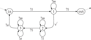
Figure 3: Cleaning gadget, assuming $\texttt{\$}\not\in{\mathsf{M}}$

For a given message alphabet ${\mathsf{M}}=\{a,\ldots\}$, the system described in Fig. 3 uses one channel (left implicit) and a new message symbol $\texttt{\$}\notin{\mathsf{M}}$. Letter $a$ in Fig. 3 is a symbol from the original message alphabet ${\mathsf{M}}$. Operations “$?m$” are used as a shorthand for all $|{\mathsf{M}}|+1$ possible reading operations over the new message alphabet ${\mathsf{M}}\cup\{\texttt{\$}\}$. The purpose of $ is to force the channel to be emptied when moving from ${{\mathtt{in}}}$ to ${{\mathtt{out}}}$.

Let $T\subseteq{\mathsf{Conf}}$ be set of configurations described by the following regular expression:

$$T=({{\mathtt{in}}},{\mathsf{M}}^{*})+(1,{\mathsf{M}}^{*}(\texttt{\$}+\varepsilon))+(2,{\mathsf{M}}^{*}\texttt{\$}^{*})+(3,\texttt{\$}^{*}a^{*})+({{\mathtt{out}}},\varepsilon)$$

Lemma 5.1

The configurations reachable from $({{\mathtt{in}}},{\mathsf{M}}^{*})$ are exactly those in $T$.

Sketch.

The left-to-right inclusion can be verified by showing that $T$ is an invariant. For instance, from configurations $({{\mathtt{in}}},{\mathsf{M}}^{*})$ only the configurations in $(1,{\mathsf{M}}^{*}(\texttt{\$}+\varepsilon))$ are reachable within one step, while from $(2,{\mathsf{M}}^{*}\texttt{\$}^{*})$ only configurations in $(3,\texttt{\$}^{*})+(2,{\mathsf{M}}^{*}\texttt{\$}^{*})$ can be reached. And so on. The other inclusion is easy to see. ∎

Constructions incorporating the gadget rely on the following property:

Lemma 5.2

For any $w\in{\mathsf{M}}^{*}$:

• If ${\mathcal{U}}$ is a scheduler for the cleaning gadget and $v\neq\varepsilon$ then $\Pr_{\mathcal{U}}\bigl{(}({{\mathtt{in}}},w)\models\Diamond({{\mathtt{out}}},v)\bigr{)}=0$.

• There is a (memoryless) scheduler ${\mathcal{U}}$ for the cleaning gadget with $\Pr_{\mathcal{U}}\bigl{(}({{\mathtt{in}}},w)\models\Diamond({{\mathtt{out}}},\varepsilon)\bigr{)}=1$.

Proof.

(a) is immediate from Lemma 5.1. To prove (b), we describe a scheduler ${\mathcal{U}}$ with the desired property. ${\mathcal{U}}$ starts from $({{\mathtt{in}}},w)$, selects the ${{\mathtt{in}}}\xrightarrow{\!\!!\texttt{\$}\!\!}1$ rule, aiming for configuration $(1,\texttt{\$})$ where $({{\mathtt{out}}},\varepsilon)$ can be reached. In case a configuration $(1,v)$ with $v\neq\texttt{\$}$ is reached, ${\mathcal{U}}$ moves from $1$ to $2$, goes back to ${{\mathtt{in}}}$ and retry. This will eventually succeed with probability $1$. ∎

Let us remark as an aside that, if one takes properties (a) and (b) above as the specification of a cleaning gadget, then it can be proved that any gadget necessarily uses “new” messages not from ${\mathsf{M}}$, like $ in our construction.

5.2 Complexity of decidable cases

We consider the decidable cases given in section 4. One problem (reachability with zero probability) is in $\mathsf{PTIME}$, and even $\mathsf{NLOGSPACE}$-complete, but all the others are non-primitive recursive, as are most decidable problems for LCS’s [Schnoebelen (2002)].

Theorem 5.3

The problem, given NPLCS ${\mathcal{N}}$, location $q$ and set $A\subseteq Q$ of locations, whether there exists a scheduler ${\mathcal{U}}$ such that $\Pr_{\mathcal{U}}\bigl{(}(q,\varepsilon)\models\Box A\bigr{)}=1$, is $\mathsf{NLOGSPACE}$-complete.

Sketch.

Lemmas 3.2 and 3.3 show that the above problem is equivalent to a reachability question in some subgraph of the control graph of ${\mathcal{L}}$. ∎

Theorem 5.4

The problem given a NPLCS ${\mathcal{N}}$, a location $q$ and a set of locations $A$, whether there exists a scheduler ${\mathcal{U}}$ satisfying $(a.1)$ (or $(a.2)$ … or $(b.3)$), is not primitive recursive.

$$\begin{array}[]{cclcccl}\text{\emph{(a.1)}}&&\Pr_{\mathcal{U}}\bigl{(}(q,\varepsilon)\models\Diamond A\bigr{)}\mathchar 8510\relax 0\text{, or}&&\text{\emph{(b.1)}}&&\Pr_{\mathcal{U}}\bigl{(}(q,\varepsilon)\models\Box\Diamond A\bigr{)}=0\text{, or}\\[3.00003pt] \text{\emph{(a.2)}}&&\Pr_{\mathcal{U}}\bigl{(}(q,\varepsilon)\models\Diamond A\bigr{)}=1\text{, or}&&\text{\emph{(b.2)}}&&\Pr_{\mathcal{U}}\bigl{(}(q,\varepsilon)\models\Box\Diamond A\bigr{)}=1\text{, or}\\[3.00003pt] \text{\emph{(a.3)}}&&\Pr_{\mathcal{U}}\bigl{(}(q,\varepsilon)\models\Diamond A\bigr{)}\mathchar 8508\relax 1\text{, or}&&\text{\emph{(b.3)}}&&\Pr_{\mathcal{U}}\bigl{(}(q,\varepsilon)\models\Box\Diamond A\bigr{)}\mathchar 8508\relax 1.\end{array}$$

In all six cases, the proof is by reducing from the control-state reachability problem for (non-probabilistic) LCS’s, known to be non-primitive recursive [Schnoebelen (2002)].

The case (a.1) is the easiest since, by Theorem 4.1, it is equivalent to the reachability of $A$ from $(q_{0},\varepsilon)$ in the underlying LCS of ${\mathcal{N}}$.

For all the other cases, except (a.3), we use the reduction illustrated in Fig. 4. Let ${\mathcal{L}}$ be a LCS with only one channel and two distinguished locations $q_{0}$ and ${{\mathtt{accept}}}$. From ${\mathcal{L}}$ we build another LCS ${\mathcal{L}}^{\prime}$ and consider the NPLCS ${\mathcal{N}}=({\mathcal{L}}^{\prime},\tau)$ for any $\tau\in(0,1)$. We now show that the control-state reachability problem in ${\mathcal{L}}$ (i.e., is ${{\mathtt{accept}}}$ reachable from $(q_{0},\varepsilon)$?) is equivalent to particular instances of our probabilistic problems for ${\mathcal{N}}$.

Figure 4: The LCS ${\mathcal{L}}^{\prime}$ associated with ${\mathcal{L}}$ in Lemma 5.5

${\mathcal{L}}^{\prime}$ uses the cleaning gadget and has one further location: ${{\mathtt{success}}}$. From every original location $r$ of ${\mathcal{L}}$, except ${{\mathtt{accept}}}$, ${\mathcal{L}}^{\prime}$ has a $\surd$-transition to ${{\mathtt{in}}}$, the input location of the cleaning gadget. There is also a transition from ${{\mathtt{out}}}$ to $q_{0}$. From ${{\mathtt{accept}}}$ there is a transition to ${{\mathtt{success}}}$ and one can loop on this latter location.

The idea of this reduction is that, if ${{\mathtt{accept}}}$ is reachable from $q_{0}$ by some path $\pi$ in ${\mathcal{L}}$, then it is possible for a scheduler to try and follow this path in ${\mathcal{L}}^{\prime}$ and, in case probabilistic losses do not comply with $\pi$, to retry as many times as it wants by returning to $q_{0}$. The cleaning gadget ensures that returning to $q_{0}$ is with empty channel. Note that the only way to visit ${{\mathtt{success}}}$ is to visit ${{\mathtt{accept}}}$ first. These general ideas are formalized in the next lemma.

Lemma 5.5

In the LCS ${\mathcal{L}}^{\prime}$, the following statements are equivalent:

• $(q_{0},\varepsilon)\xrightarrow{\!\!*\!\!}{\mathit{Prom}}(\{{{\mathtt{success}}}\})$,

• $q_{0}\in{\mathit{Prom}}(\{{{\mathtt{success}}}\})$,

• $(q_{0},\varepsilon)\xrightarrow{\!\!*\!\!}{{\mathtt{success}}}$,

• $(q_{0},\varepsilon)\xrightarrow{\!\!*\!\!}{{\mathtt{accept}}}$,

• $(q_{0},\varepsilon)\xrightarrow{\!\!*\!\!}_{[{\mathcal{L}}]}{{\mathtt{accept}}}$,

• $q_{0}\in{\mathit{Safe}}({\mathit{Prom}}(\{{{\mathtt{success}}}\}))$,

• $(q_{0},\varepsilon)\xrightarrow{\!\!*\!\!}{\mathit{Safe}}({\mathit{Prom}}(\{{{\mathtt{success}}}\}))$.

Here “$(q_{0},\varepsilon)\xrightarrow{\!\!*\!\!}_{[{\mathcal{L}}]}\cdots$” means that the path only visits original locations from ${\mathcal{L}}$.

Proof.

(i) $\Longrightarrow$ (ii): Assume $(q_{0},\varepsilon)\xrightarrow{\!\!*\!\!}{\mathit{Prom}}(\{{{\mathtt{success}}}\})$ and let $(q_{0},\varepsilon)\to(q_{1},w_{1})\to\cdots\to(q_{m},w_{m})$ with $q_{m}\in{\mathit{Prom}}(\{{{\mathtt{success}}}\})$ be a witness (simple) path. From any $q_{i}\neq{{\mathtt{success}}}$ along this path one may reach $(q_{0},\varepsilon)$ via the cleaning gadget. Hence $(q_{i},\varepsilon)\xrightarrow{\!\!*\!\!}{\mathit{Prom}}({{\mathtt{success}}})$. All locations along the path from $(q_{0},\varepsilon)$ to ${\mathit{Prom}}(\{{{\mathtt{success}}}\})$ satisfies this property, hence we have $q_{0}\in{\mathit{Prom}}(\{{{\mathtt{success}}}\})$.

(ii) $\Longrightarrow$ (iii): by definition of ${\mathit{Prom}}(.)$.

(iii) $\Longrightarrow$ (iv): obvious.

(iv) $\Longrightarrow$ (v): Assume $\pi$ is a path from $(q_{0},\varepsilon)$ to ${{\mathtt{accept}}}$. If this path steps out of ${\mathcal{L}}$ then it can only go to the cleaning gadget. From there the only exit back to ${\mathcal{L}}$ is via $(q_{0},\varepsilon)$ (Lemma 5.2.(a)), looping back to a previously visited configuration. Thus if $\pi$ is a simple path, it stays inside ${\mathcal{L}}$.

(v) $\Longrightarrow$ (vi): suppose $(q_{0},\varepsilon)\xrightarrow{\!\!*\!\!}_{[{\mathcal{L}}]}{{\mathtt{accept}}}$. Then $(q_{0},\varepsilon)\xrightarrow{\!\!*\!\!}{{\mathtt{success}}}$ and $s\xrightarrow{\!\!*\!\!}{{\mathtt{success}}}$ for all configurations of ${\mathcal{L}}^{\prime}$, either because $s$ is already some $({{\mathtt{success}}},w)$, or because $s$ can reach $(q_{0},\varepsilon)$ via the cleaning gadget. As a consequence, all locations of ${\mathcal{L}}^{\prime}$ are in ${\mathit{Prom}}(\{{{\mathtt{success}}}\})$, and then in ${\mathit{Safe}}({\mathit{Prom}}(\{{{\mathtt{success}}}\}))$.

(vi) $\Longrightarrow$ (vii): trivial.

(vii) $\Longrightarrow$ (i): obvious because ${\mathit{Safe}}(A)\subseteq A$ for any set $A$ of locations. ∎

Using Lemma 5.5 and characterizations given by Theorems 4.1 and 4.7 we have:

$$\exists{\mathcal{U}}\ \Pr\nolimits_{\mathcal{U}}\bigl{(}(q_{0},\varepsilon)\models\Diamond{{\mathtt{success}}}\bigr{)}=1 \text{ iff }q_{0}\in{\mathit{Prom}}(\{{{\mathtt{success}}}\})$$ (a.2)

$$\text{ iff }\text{in ${\mathcal{L}}$, }q_{0}\xrightarrow{\!\!*\!\!}{{\mathtt{accept}}}.$$

$$\exists{\mathcal{U}}\ \Pr\nolimits_{\mathcal{U}}\bigl{(}(q_{0},\varepsilon)\models\Box\Diamond{{\mathtt{success}}}\bigr{)}=1 \text{ iff }q_{0}\in{\mathit{Safe}}({\mathit{Prom}}(\{{{\mathtt{success}}}\}))$$ (b.2)

$$\text{ iff }\text{in ${\mathcal{L}}$, }q_{0}\xrightarrow{\!\!*\!\!}{{\mathtt{accept}}}.$$

$$\exists{\mathcal{U}}\ \Pr\nolimits_{\mathcal{U}}\bigl{(}(q_{0},\varepsilon)\models\Box\Diamond\neg{{\mathtt{success}}}\bigr{)}=0 \text{ iff }q_{0}\in{\mathit{Prom}}({\mathit{Safe}}(Q\setminus\{{{\mathtt{success}}}\}))$$ (b.1)

$$\text{ iff }\text{in ${\mathcal{L}}$, }q_{0}\xrightarrow{\!\!*\!\!}{{\mathtt{accept}}}.$$

$$\exists{\mathcal{U}}\ \Pr\nolimits_{\mathcal{U}}\bigl{(}(q_{0},\varepsilon)\models\Box\Diamond\neg{{\mathtt{success}}}\bigr{)}\mathchar 8508\relax 1 \text{ iff }q_{0}\xrightarrow{\!\!*\!\!}Q\setminus\{{{\mathtt{success}}}\}$$ (b.3)

$$\text{ iff }\text{in ${\mathcal{L}}$, }q_{0}\xrightarrow{\!\!*\!\!}{{\mathtt{accept}}}.$$

Thus, $q_{0}\xrightarrow{\!\!*\!\!}{{\mathtt{accept}}}$, a non-primitive recursive problem, reduces to instances of $(a.1)$, $(b.2)$, $(b.1)$ and $(b.3)$.

We now prove case (a.3) of Theorem 5.4, using the reduction described in Fig. 5.

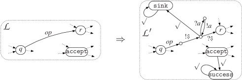
Figure 5: Associating ${\mathcal{L}}^{\prime}$ with an arbitrary LCS ${\mathcal{L}}$ for case $(a.3)$

Here, with some LCS ${\mathcal{L}}$ as before, we associate an LCS ${\mathcal{L}}^{\prime}$ by adding two special locations ${{\mathtt{sink}}}$ and ${{\mathtt{success}}}$. As in the previous reduction, ${{\mathtt{success}}}$ is directly reachable from ${{\mathtt{accept}}}$ by an internal action $\surd$, and one can loop on ${{\mathtt{success}}}$.

Now, each transition rule $\delta:q\xrightarrow{\!\!{\mathit{op}}\!\!}r$ in ${\mathcal{L}}$ is translated in ${\mathcal{L}}^{\prime}$ under the form $q\xrightarrow{\!\!{\mathit{op}}\!\!}l_{\delta}\xrightarrow{\!\!!\texttt{\$}\!\!}l^{\prime}_{\delta}\xrightarrow{\!\!?\texttt{\$}\!\!}r$, using two intermediate locations $l_{\delta}$ and $l^{\prime}_{\delta}$, and a new message $\texttt{\$}\not\in{\mathsf{M}}$. Thus, moving from $q$ to $r$ in ${\mathcal{L}}^{\prime}$ requires that one removes the extra $ that has just been inserted. This is obtained by a full rotation of the channel contents, using extra rules $l^{\prime}_{\delta}\xrightarrow{\!\!?a\!\!}\_\xrightarrow{\!\!!a\!\!}l^{\prime}_{\delta}$ that exist for each $a\in{\mathsf{M}}$. Finally, in case of deadlocks induced by message losses, one can go to the ${{\mathtt{sink}}}$ location.

The purpose of this reduction is to ensure that ${{\mathtt{accept}}}$ and ${{\mathtt{success}}}$ are the only locations from which one can surely, i.e., with probability one, reach ${{\mathtt{success}}}$. For all other locations, the channel may become empty along the way to ${{\mathtt{accept}}}$, forcing the system to go to ${{\mathtt{sink}}}$.

Lemma 5.6

In ${\mathcal{N}}=({\mathcal{L}}^{\prime},\tau)$ the following assertions are equivalent:

1. $\exists{\mathcal{U}}\ \Pr_{\mathcal{U}}\bigl{(}(q_{0},\varepsilon)\models\Diamond{{\mathtt{sink}}}\bigr{)}\mathchar 8508\relax 1$,

2. $q_{0}\xrightarrow{\!\!*\!\!}_{[\neg{{\mathtt{sink}}}]}{\mathit{Safe}}(Q\setminus\{{{\mathtt{sink}}}\})$,

3. $q_{0}\xrightarrow{\!\!*\!\!}_{[\neg{{\mathtt{sink}}}]}\{{{\mathtt{accept}}},{{\mathtt{success}}}\}$,

4. $q_{0}\xrightarrow{\!\!*\!\!}_{[{\mathcal{L}}]}\{{{\mathtt{accept}}}\}$.

where here again “$(q_{0},\varepsilon)\xrightarrow{\!\!*\!\!}_{[{\mathcal{L}}]}\cdots$” means that the path only visits original locations from ${\mathcal{L}}$.

Proof.

The equivalence between (1) and (2) is given by case (c) of Theorem 4.1. Then we show that ${\mathit{Safe}}(Q\setminus\{{{\mathtt{sink}}}\})=\{{{\mathtt{accept}}},{{\mathtt{success}}}\}$. First $\{{{\mathtt{accept}}},{{\mathtt{success}}}\}\subseteq{\mathit{Safe}}(Q\setminus\{{{\mathtt{sink}}}\})$ because from ${{\mathtt{accept}}}$ and ${{\mathtt{success}}}$ one can loop forever in ${{\mathtt{success}}}$ which is in $Q\setminus\{{{\mathtt{sink}}}\}$. On the other hand, if we consider another location $q$ different from ${{\mathtt{sink}}}$ (neither ${{\mathtt{success}}}$ nor ${{\mathtt{accept}}}$) because of the reading operation between $l^{\prime}_{\delta}$ and $r$, there is a non-zero probability for the system to lose the message $ and be forced to go to ${{\mathtt{sink}}}$. Hence ${\mathit{Safe}}(Q\setminus\{{{\mathtt{sink}}}\})$ is exactly $\{{{\mathtt{accept}}},{{\mathtt{success}}}\}$. Equivalences of (2) with (3) and (4) follow from this equality. ∎

Thus the non-primitive recursive problem “does $(q_{0},\varepsilon)\xrightarrow{\!\!*\!\!}{{\mathtt{accept}}}$” reduces to a special instance of problem $(a.3)$ in Theorem 5.4.

5.3 Undecidability

5.3.1 An undecidability result for repeated eventually properties

We will now combine the cleaning gadget with an arbitrary lossy channel system to get a reduction from the boundedness problem for LCS’s to the question whether a single Büchi constraint $\Box\Diamond A$ holds with positive probability under some scheduler. Recall that an LCS ${\mathcal{L}}$ is bounded (also space-bounded) for a given a starting configuration if the set of reachable configurations is finite.

Theorem 5.7 ((Single Büchi property, positive probability))

The problem,
given ${\mathcal{N}}$ a NPLCS, $q$ a location, and $A$ a set of locations, whether there exists a scheduler ${\mathcal{U}}$ such that $\Pr_{\mathcal{U}}\bigl{(}(q,\varepsilon)\models\Box\Diamond A\bigr{)}\mathchar 8510\relax 0$, is undecidable.

The remainder of this subsection is concerned with the proof of Theorem 5.7. Let ${\mathcal{L}}=(Q,\{c\},{\mathsf{M}},\Delta)$ be a LCS with a single channel $c$ and a designated initial configuration $(q,\varepsilon)$. We modify ${\mathcal{L}}$ by adding the cleaning gadget and two locations: ${{\mathtt{success}}}$ and ${{\mathtt{sink}}}$. We also add rules allowing to jump from every “original” location in $Q$ to ${{\mathtt{retry}}}$ or ${{\mathtt{success}}}$. When in ${{\mathtt{success}}}$, one can move to ${{\mathtt{retry}}}$ with a read or move to ${{\mathtt{sink}}}$ which cannot be left. When in ${{\mathtt{retry}}}$, one can go back to $(q,\varepsilon)$ through the cleaning gadget. The whole construction is depicted in Fig. 6.

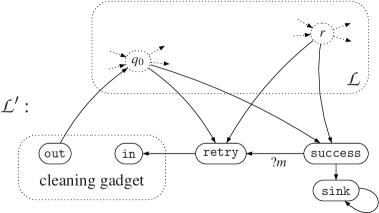
Figure 6: The LCS ${\mathcal{L}}^{\prime}$ associated with ${\mathcal{L}}$ in proof of Theorem 5.7

Let ${\mathcal{L}}^{\prime}$ be the resulting LCS which we consider as an NPLCS with some fault rate $\tau$: ${\mathcal{N}}=({\mathcal{L}}^{\prime},\tau)$. Since the cleaning gadget lets one go back to the initial configuration of ${\mathcal{L}}$, any behavior of ${\mathcal{L}}^{\prime}$ is a succession of behaviors of ${\mathcal{L}}$ separated by visits to the additional locations. The idea of this construction is the following: if ${\mathcal{L}}$ is bounded, then even the best scheduler cannot visit ${{\mathtt{success}}}$ infinitely often without ending up in ${{\mathtt{sink}}}$ almost surely. However, if the system ${\mathcal{L}}$ is bounded, some infinite memory scheduler can achieve this. These ideas are formalized in Propositions 5.8 and 5.9.

Proposition 5.8

Assume that ${\mathcal{L}}$ starting from $(q,\varepsilon)$ is bounded. Then, for all schedulers ${\mathcal{U}}$ for ${\mathcal{N}}=({\mathcal{L}}^{\prime},\tau)$, $\Pr_{\mathcal{U}}\bigl{(}(q,\varepsilon)\models\Box\Diamond{{{\mathtt{success}}}}\bigr{)}=0$.

Proof.

Let ${\mathcal{U}}$ be any scheduler for ${\mathcal{N}}$ and consider the ${\mathcal{U}}$-paths that visit ${{\mathtt{success}}}$ infinitely often. Let $\pi$ be one such path: either $\pi$ jumps from ${\mathcal{L}}$ to ${{\mathtt{success}}}$ infinitely many times, or it ends up in ${{\mathtt{sink}}}$. In the last case, $\pi$ does not satisfy $\Box\Diamond{{\mathtt{success}}}$. In the first case, and since ${\mathcal{L}}$ is bounded, $\pi$ can only jump to ${{\mathtt{success}}}$ from finitely many different configurations. Hence, for each such jump, the probability that it ends in $({{\mathtt{success}}},\varepsilon)$ is at least $\tau^{m}$, where $m$ is the size of the largest reachable configuration in ${\mathcal{L}}$. Therefore, the configurations $({{\mathtt{success}}},\varepsilon)$ will be visited almost surely. As only the transition rule

$${{\mathtt{success}}}\xrightarrow{\!\!\surd\!\!}{{\mathtt{sink}}}$$

is enabled in $({{\mathtt{success}}},\varepsilon)$, with probability 1 the location ${{\mathtt{sink}}}$ is eventually reached. Since ${{\mathtt{success}}}$ is not reachable from ${{\mathtt{sink}}}$, the property $\Box\Diamond{{\mathtt{success}}}$ holds with zero probability. ∎

Proposition 5.9

Assume that ${\mathcal{L}}$ starting from $(q,\varepsilon)$ is unbounded. Then, there exists a scheduler ${\mathcal{U}}$ for ${\mathcal{N}}=({\mathcal{L}}^{\prime},\tau)$ with $\Pr_{\mathcal{U}}\bigl{(}(q,\varepsilon)\models\Box\Diamond{{{\mathtt{success}}}}\bigr{)}\mathchar 8510\relax 0$.

Proof.

We describe the required scheduler ${\mathcal{U}}$. Because ${\mathcal{L}}$ is unbounded, we can pick a sequence $\bigl{(}(r_{n},w_{n})\bigr{)}_{n=1,2,\ldots}$ of reachable configurations such that $|w_{n}|\geq n$. The scheduler works in phases numbered $1,2,\ldots$ When phase $n$ starts, ${\mathcal{U}}$ is in the initial configuration $(q,\varepsilon)$ and tries to reach $(r_{n},w_{n})$. In principle, this can be achieved (since $(r_{n},w_{n})$ is reachable), but it requires that the right messages are lost at the right times. These losses are probabilistic and ${\mathcal{U}}$ cannot control them. Thus ${\mathcal{U}}$ aims for $(r_{n},w_{n})$ and hopes for the best. It goes on according to plan as long as losses occur as hoped. When a “wrong” loss occurs, ${\mathcal{U}}$ resigns temporarily, jumps directly to ${{\mathtt{retry}}}$, reaches the initial configuration $(q,\varepsilon)$ via the cleaning gadget, and then tries again to reach $(r_{n},w_{n})$. When $(r_{n},w_{n})$ is eventually reached (which will happen almost surely given enough retries), ${\mathcal{U}}$ jumps to ${{\mathtt{success}}}$, from there to ${{\mathtt{retry}}}$, and initiates phase $n+1$. With these successive phases, ${\mathcal{U}}$ tries to visit ${{\mathtt{success}}}$ (and ${{\mathtt{retry}}}$) an infinite number of times. We now show that it succeeds with nonzero probability.

When moving from configuration $(r_{n},w_{n})$ to location ${{\mathtt{success}}}$, there is a nonzero probability ${\textbf{P}}_{\mathit{lost}}(w_{n},\varepsilon)$ that all messages in the channel are lost, leaving us in $({{\mathtt{success}}},\varepsilon)$. When this happens, ${\mathcal{U}}$ is not able to initiate phase $n+1$ (moving from ${{\mathtt{success}}}$ to ${{\mathtt{retry}}}$ requires a nonempty channel). Instead ${\mathcal{U}}$ will move to ${{\mathtt{sink}}}$ and stay there forever. However, the probability for this exceptional behavior is strictly less than 1, as we have:

$$\Pr\nolimits_{\mathcal{U}}\bigl{(}(q,\varepsilon)\models\Box\Diamond{{\mathtt{success}}}\bigr{)}=\prod_{n=1}^{\infty}(1-{\textbf{P}}_{\mathit{lost}}(w_{n},\varepsilon))\geq\prod_{n=1}^{\infty}(1-\tau^{n})\mathchar 8510\relax 0.$$

∎

Observe that the scheduler we constructed is recursive but not finite-memory (since it records the index of the current phase).

Remark 5.10.

Proposition 5.9 can be strengthened: if ${\mathcal{L}}$ is unbounded, then for all constant $c<1$, there exists a scheduler ${\mathcal{U}}$ such that $\Pr_{\mathcal{U}}\bigl{(}(q,\varepsilon)\models\Box\Diamond{{{\mathtt{success}}}}\bigr{)}\mathchar 8510\relax c$.

Corollary 5.11

Let ${\mathcal{L}}$ be a LCS. Then, ${\mathcal{L}}$ is unbounded if and only if there exists a scheduler ${\mathcal{U}}$ for ${\mathcal{N}}=({\mathcal{L}}^{\prime},\tau)$ such that $\Pr_{\mathcal{U}}\bigl{(}(q,\varepsilon)\models\Box\Diamond{{{\mathtt{success}}}}\bigr{)}\mathchar 8510\relax 0$.

This proves Theorem 5.7 since it is undecidable whether a given LCS is bounded [Mayr (2003)].

By duality we obtain the undecidability of the problem to check whether $\Pr_{\mathcal{U}}\bigl{(}(q,\varepsilon)\models\Diamond\Box A\bigr{)}=1$ for all schedulers ${\mathcal{U}}$ for a given NPLCS ${\mathcal{N}}$.

5.3.2 Other undecidability results

We now discuss the decidability of the problem which asks for a scheduler ${\mathcal{U}}$ where $\Pr_{\mathcal{U}}\bigl{(}(q,\varepsilon)\models\varphi\bigr{)}$ is 1, $\mathchar 8508\relax 1$, $=0$ or $\mathchar 8510\relax 0$ and where $\varphi$ is an LTL-formula. We begin with the special case of a strong fairness (Streett condition) $\varphi=\bigwedge_{1\leq i\leq n}(\Box\Diamond A_{i}\Rightarrow\Box\Diamond B_{i})$. We will see that all variants of the qualitative model checking problem for such Streett conditions are undecidable when ranging over the full class of schedulers. In particular, this yields the undecidability of the LTL model checking problem when considering all schedulers. However, when we shrink our attention to finite-memory schedulers qualitative model checking is decidable for properties specified by Streett conditions or even $\omega$-regular formulas.

We first establish the undecidability results when ranging over all schedulers. In fact, already a special kind of Streett properties with the probabilistic satisfaction criterion “almost surely” cannot be treated algorithmically:

Lemma 5.12

The problem, given NPLCS ${\mathcal{N}}$, sets of locations $A,B\subseteq Q$, and location $q\in Q$, whether there exists a scheduler ${\mathcal{U}}$ with

$$\Pr\nolimits_{\mathcal{U}}\bigl{(}(q,\varepsilon)\models\Box\Diamond B\wedge\Diamond\Box A)\bigr{)}=1,$$

is undecidable.

Proof.

The proof is again by a reduction from the boundedness problem for LCS as in section 5.3.1. Let ${\mathcal{L}}$ be an LCS. We build a new LCS ${\mathcal{L}}^{\prime}$ by combining ${\mathcal{L}}$ with the cleaning gadget as shown in Fig. 7 (this is a variant of the previous construction). Let ${\mathcal{N}}=({\mathcal{L}}^{\prime},\tau)$.

Figure 7: The LCS ${\mathcal{L}}^{\prime}$ associated with ${\mathcal{L}}$ in proof of Lemma 5.12

There exists a scheduler ${\mathcal{U}}$ for ${\mathcal{N}}$ with $\Pr_{\mathcal{U}}\bigl{(}(q_{0},\varepsilon)\models\Box\Diamond{{\mathtt{success}}}\wedge\Diamond\Box\neg{{\mathtt{fail}}}\bigr{)}=1$ iff ${\mathcal{L}}$ is unbounded (starting from $(q_{0},\varepsilon)$).

For these two constructions, the “same” scheduler is used in the positive cases. For the second construction, the proof for the positive case observes that

$$\Pr\nolimits_{\mathcal{U}}\bigl{(}(q_{0},\varepsilon)\models\Box\Diamond{{\mathtt{success}}}\wedge\Diamond\Box\neg{{\mathtt{fail}}}\bigr{)}=\lim_{n\rightarrow\infty}\prod_{k=n}^{\infty}(1-\tau^{k})=1.$$

where $n$ stands for the phase number from which ${{\mathtt{fail}}}$ will not be visited again. ∎

Theorem 5.13 ((Streett properties))

For the qualitative properties (a), …, (d) below, the problem, given a NPLCS ${\mathcal{N}}$, location $q\in Q$, and $2n$ sets of locations $A_{1},B_{1},\ldots,$ $A_{n},B_{n}\subseteq Q$, whether there exists a scheduler ${\mathcal{U}}$ such that

1. $\Pr_{\mathcal{U}}\bigl{(}(q,\varepsilon)\models\bigwedge\limits_{i=1}^{n}(\Box\Diamond A_{i}\Rightarrow\Box\Diamond B_{i})\bigr{)}\mathchar 8510\relax 0$,

2. $\Pr_{\mathcal{U}}\bigl{(}(q,\varepsilon)\models\bigwedge\limits_{i=1}^{n}(\Box\Diamond A_{i}\Rightarrow\Box\Diamond B_{i})\bigr{)}\mathchar 8508\relax 1$,

3. $\Pr_{\mathcal{U}}\bigl{(}(q,\varepsilon)\models\bigwedge\limits_{i=1}^{n}(\Box\Diamond A_{i}\Rightarrow\Box\Diamond B_{i})\bigr{)}=1$,

4. $\Pr_{\mathcal{U}}\bigl{(}(q,\varepsilon)\models\bigwedge\limits_{i=1}^{n}(\Box\Diamond A_{i}\Rightarrow\Box\Diamond B_{i})\bigr{)}=0$,

is undecidable.

Proof.

1. follows immediately from Theorem 5.7 as $\bigwedge_{i=1}^{n}(\Box\Diamond A_{i}\Rightarrow\Box\Diamond B_{i})$ agrees with $\Box\Diamond B$ if we take $n=1$, $A_{1}=Q$ and $B_{1}=B$.

2. We show that already the question whether there is some scheduler ${\mathcal{U}}$ with $\Pr_{\mathcal{U}}\bigl{(}(q,\varepsilon)\models\Box\Diamond A\Rightarrow\Box\Diamond B\bigr{)}\mathchar 8508\relax 1$ is undecidable where $A$ and $B$ are sets of locations. This follows from Theorem 5.7 and the fact that for $B=\emptyset$

   		$\Pr_{\mathcal{U}}\bigl{(}(q,\varepsilon)\models\Box\Diamond A\Rightarrow\Box\Diamond B\bigr{)}\mathchar 8508\relax 1$
   iff		$\Pr_{\mathcal{U}}\bigl{(}(q,\varepsilon)\models\neg(\Box\Diamond A\Rightarrow\Box\Diamond B)\bigr{)}\mathchar 8510\relax 0$
   iff		$\Pr_{\mathcal{U}}\bigl{(}(q,\varepsilon)\models\Box\Diamond A\wedge\underbrace{\Diamond\Box(Q\setminus B)}_{\equiv{\mathsf{true}}~{}\text{since $B=\emptyset$}}\bigr{)}\mathchar 8510\relax 0$
   iff		$\Pr_{\mathcal{U}}\bigl{(}(q,\varepsilon)\models\Box\Diamond A\bigr{)}\mathchar 8510\relax 0$.

3. follows by Lemma 5.12 with $n=2$, $A_{1}=Q$, $B_{1}=B$, $A_{2}=Q\setminus A$ and $B_{2}=\emptyset$ which yields

   $$\bigwedge\limits_{1\leq i\leq n}\bigl{(}\Box\Diamond A_{i}\Rightarrow\Box\Diamond B_{i}\bigr{)} \;\;\equiv\;\;\bigl{(}\underbrace{\Box\Diamond Q}_{\equiv{\mathsf{true}}}\Rightarrow\Box\Diamond B\bigr{)}\>\wedge\>\bigl{(}\Box\Diamond(Q\setminus A)\Rightarrow\underbrace{\Box\Diamond\emptyset}_{\equiv{\mathsf{false}}}\bigr{)}$$

   $$\;\;\equiv\;\;\Box\Diamond B\>\wedge\>\Diamond\Box A.$$

4. We show the undecidability of the question whether $\Pr_{\mathcal{U}}\bigl{(}(q,\varepsilon)\models\Box\Diamond A\Rightarrow\Box\Diamond B\bigr{)}=0$ for some ${\mathcal{U}}$ where $A,B\subseteq Q$ are given sets of locations. This follows from Lemma 5.12 and the fact that

   		$\Pr_{\mathcal{U}}\bigl{(}(q,\varepsilon)\models\Box\Diamond A\Rightarrow\Box\Diamond B\bigr{)}=0$
   iff		$\Pr_{\mathcal{U}}\bigl{(}(q,\varepsilon)\models\neg(\Box\Diamond A\Rightarrow\Box\Diamond B)\bigr{)}=1$
   iff		$\Pr_{\mathcal{U}}\bigl{(}(q,\varepsilon)\models\Box\Diamond A\wedge\Diamond\Box(Q\setminus B)\bigr{)}=1$.

∎

Figure 8 summarizes the decidability and undecidability results obtained so far.

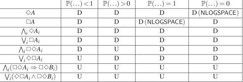
Figure 8: (Un)Decidability of qualitative verification

6 Restriction to finite-memory schedulers

In all decidable cases of section 4, finite-memory schedulers are sufficient. In this section we consider the problems of section 5, considering only finite-memory schedulers. With this restriction, all problems are decidable.

We first give an immediate property of finite-memory schedulers which will be used in the whole section.

Proposition 6.1

For any finite-memory scheduler ${\mathcal{U}}$ and any location $q$ we have:

1. If $p$ is a location, $u$ a mode in ${\mathcal{U}}$ and if $T$ denotes the set of all configurations $t$ that are reachable from $(p,\varepsilon)_{u}$ by ${\mathcal{U}}$ then

   $$\Pr\nolimits_{\mathcal{U}}\bigl{(}(q,\varepsilon)\models\Box\Diamond(p,\varepsilon)_{u}\bigr{)}=\Pr\nolimits_{\mathcal{U}}\bigl{(}(q,\varepsilon)\models\bigwedge_{s\in T}\Box\Diamond s\bigr{)}$$

2. $\Pr\nolimits_{\mathcal{U}}\bigl{(}(q,\varepsilon)\models\Box\Diamond A\bigr{)}=\Pr\nolimits_{\mathcal{U}}\bigl{(}(q,\varepsilon)\models\Box\Diamond A_{\varepsilon}\bigr{)}$.

Proof.

(a) If configuration $s_{u}$ in the Markov chain ${\mathit{MC}}_{\mathcal{U}}$ is visited infinitely often then almost surely all direct successors of $s_{u}$ are visited infinitely often too. We now may repeat this argument for the direct successors of the direct successors of $s_{u}$, and so on. We obtain that almost surely all configurations that are reachable from $s_{u}$ are visited infinitely often, provided that $s_{u}$ is visited infinitely often.

(b) follows from (a) using the fact that the set of all $(p,\varepsilon)_{u}$ for $p$ a location and $u$ a mode of ${\mathcal{U}}$, is a finite attractor, and observing that if $(a,w)$ is reachable within one step from configuration $s$ then so is $(a,\varepsilon)$ as all messages can be lost. ∎

Observe that the existence of a scheduler ${\mathcal{U}}$ for which a B chi property holds with positive probability, does not imply the existence of a finite-memory scheduler with the same property. This is a consequence of Theorem 5.7 and the next Theorem (6.2).

Theorem 6.2 ((Generalized Büchi, positive probability))

The problem, given NPLCS ${\mathcal{N}}$, location $q\in Q$, and sets of locations $A_{1},\ldots,A_{n}\subseteq Q$, whether there exists a finite-memory scheduler ${\mathcal{U}}$ such that $\Pr_{\mathcal{U}}\bigl{(}(q,\varepsilon)\models\bigwedge_{1\leq i\leq n}\Box\Diamond A_{i}\bigr{)}\mathchar 8510\relax 0$, is decidable.

Proof.

We show that the following statements (1) and (2) are equivalent:

1. there exists a finite-memory scheduler ${\mathcal{U}}$ such that $\Pr_{\mathcal{U}}\bigl{(}(q,\varepsilon)\models\bigwedge\limits_{1\leq i\leq n}\Box\Diamond A_{i}\bigr{)}\mathchar 8510\relax 0$.

2. there exists a location $x\in Q$ such that

   1. $(q,\varepsilon)\xrightarrow{\!\!*\!\!}(x,\varepsilon)$

   2. there is a finite-memory scheduler ${\mathcal{V}}$ with $\Pr_{{\mathcal{V}}}\bigl{(}(x,\varepsilon)\models\bigwedge\limits_{1\leq i\leq n}\Box\Diamond A_{i}\bigr{)}=1$

This will prove Theorem 6.2 since by Theorem 4.7 (a), there is an algorithmic way to compute the set $X$ of locations $x$ such that $\Pr_{{\mathcal{V}}}\bigl{(}(x,\varepsilon)\models\bigwedge_{1\leq i\leq n}\Box\Diamond A_{i}\bigr{)}=1$ for some (finite-memory) scheduler ${\mathcal{V}}$. We then may check (2.1) by an ordinary reachability analysis in the underlying LCS.

Let us show the equivalence of (1) and (2).

(1) $\Longrightarrow$ (2): Let ${\mathcal{U}}$ be a finite-memory scheduler as in (1). The finite-attractor property and Proposition 6.1 yield that there is some location $x$ and mode $u$ of ${\mathcal{U}}$ with

$$\Pr\nolimits_{\mathcal{U}}\bigl{(}(q,\varepsilon)\models\bigwedge_{1\leq i\leq n}\Box\Diamond A_{i}\wedge\bigwedge_{t\in T}\Box\Diamond t\bigr{)}\mathchar 8510\relax 0$$

where $T$ is the set of configurations that are reachable from $(x,\varepsilon)_{u}$ under ${\mathcal{U}}$. Using definition of $T$, this yields $T\cap A_{i}\neq\emptyset$ for $1\leq i\leq n$. Thus, scheduler ${\mathcal{U}}$ starting in $(x,\varepsilon)$ in mode $u$ visits almost surely any configuration in $T$ infinitely often. Hence, it visits any set $A_{i}$ for $i=1,\ldots,n$, infinitely often (with probability one). That is:

$$\Pr\nolimits_{\mathcal{U}}\bigl{(}(x,\varepsilon)_{u}\models\bigwedge_{1\leq i\leq n}\Box\Diamond A_{i}\bigr{)}=1,$$

and (2) holds.

(2) $\Longrightarrow$ (1): Let $q$, $x$ and ${\mathcal{V}}$ be as in (2). We define ${\mathcal{U}}$ as the finite-memory scheduler that generates with positive probability a path from $(q,\varepsilon)$ to $(x,\varepsilon)$ and behaves as ${\mathcal{V}}$ from $(x,\varepsilon)$ on. Clearly, we then have $\Pr_{\mathcal{U}}\bigl{(}(q,\varepsilon)\models\bigwedge_{1\leq i\leq n}\Box\Diamond A_{i}\bigr{)}\mathchar 8510\relax 0$. ∎

We now present algorithms for the four variants of qualitative model checking of Streett properties for NPLCS’s when ranging over finite-memory schedulers.

Theorem 6.3 ((Streett properties))

For qualitative properties (a), …, (d), the problem, given NPLCS ${\mathcal{N}}$, location $q\in Q$, and $2n$ sets of locations $A_{1},B_{1},\ldots,A_{n},B_{n}\subseteq Q$, whether there exists a finite-memory scheduler ${\mathcal{U}}$ satisfying

• $\Pr_{\mathcal{U}}\bigl{(}(q,\varepsilon)\models\bigwedge\limits_{1\leq i\leq n}(\Box\Diamond A_{i}\Rightarrow\Box\Diamond B_{i})\bigr{)}\mathchar 8508\relax 1$,

• $\Pr_{\mathcal{U}}\bigl{(}(q,\varepsilon)\models\bigwedge\limits_{1\leq i\leq n}(\Box\Diamond A_{i}\Rightarrow\Box\Diamond B_{i})\bigr{)}\mathchar 8510\relax 0$,

• $\Pr_{\mathcal{U}}\bigl{(}(q,\varepsilon)\models\bigwedge\limits_{1\leq i\leq n}(\Box\Diamond A_{i}\Rightarrow\Box\Diamond B_{i})\bigr{)}=1$,

• $\Pr_{\mathcal{U}}\bigl{(}(q,\varepsilon)\models\bigwedge\limits_{1\leq i\leq n}(\Box\Diamond A_{i}\Rightarrow\Box\Diamond B_{i})\bigr{)}=0$,

is decidable.

We prove each assertion in the rest of this section.

ad (a) of Theorem 6.3: $\Pr_{\mathcal{U}}\bigl{(}(q,\varepsilon)\models\bigwedge\limits_{1\leq i\leq n}(\Box\Diamond A_{i}\Rightarrow\Box\Diamond B_{i})\bigr{)}\mathchar 8508\relax 1$.

Let us consider the dual problem whether, for all finite-memory schedulers ${\mathcal{U}}$,

$$\Pr\nolimits_{\mathcal{U}}\bigl{(}(q,\varepsilon)\models\bigwedge\limits_{i=1}^{n}(\Box\Diamond A_{i}\Rightarrow\Box\Diamond B_{i})\bigr{)}=1$$

Clearly, the above holds iff

$$\Pr\nolimits_{\mathcal{U}}\bigl{(}(q,\varepsilon)\models\Box\Diamond A_{i}\Rightarrow\Box\Diamond B_{i}\bigr{)}=1$$

for all finite-memory schedulers ${\mathcal{U}}$ and all indices $i=1,\ldots,n$. Thus, it suffices to present an algorithm that solves the problem whether $\Pr_{\mathcal{U}}\bigl{(}(q,\varepsilon)\models\Box\Diamond A\Rightarrow\Box\Diamond B\bigr{)}=1$ for all finite-memory schedulers ${\mathcal{U}}$ where $A$ and $B$ are given sets of locations. The latter is equivalent to the non-existence of a finite-memory scheduler ${\mathcal{U}}$ such that

$$\Pr\nolimits_{\mathcal{U}}\bigl{(}(q,\varepsilon)\models\Box\Diamond A\wedge\Diamond\Box(Q\setminus B)\bigr{)}\mathchar 8510\relax 0.$$

We now explain how to check this condition algorithmically. Let ${\mathcal{N}}^{\prime}$ be the NPLCS that arises from ${\mathcal{N}}$ by removing all locations $b\in B$. To ensure that any configuration has at least one outgoing transition, we add a new location ${{\mathtt{fail}}}$ with

• a self-loop ${{\mathtt{fail}}}\xrightarrow{\!\!\surd\!\!}{{\mathtt{fail}}}$ and

• transition rules $p\xrightarrow{\!\!{\mathit{op}}\!\!}{{\mathtt{fail}}}$ if $p\xrightarrow{\!\!{\mathit{op}}\!\!}b$ for some location $b\in B$.

Using Theorem 6.2, we can compute the set $P$ of locations $p\in Q\setminus B$ such that there is a finite-memory scheduler ${\mathcal{U}}^{\prime}$ for ${\mathcal{N}}^{\prime}$ with $\Pr_{{\mathcal{U}}^{\prime}}\bigl{(}(p,\varepsilon)\models\Box\Diamond A\bigr{)}\mathchar 8510\relax 0$. That is,

$$P=\left\{p\in Q\left|\begin{array}[]{c}\text{there is some finite-memory scheduler ${\mathcal{U}}$ for ${\mathcal{N}}$}\\ \text{with }\Pr_{{\mathcal{U}}}\bigl{(}(p,\varepsilon)\models\Box\Diamond A\wedge\Box\neg B\bigr{)}\mathchar 8510\relax 0\end{array}\right.\right\}.$$

We show the equivalence of the following two statements:

(1)

$\Pr_{\mathcal{U}}\bigl{(}(q,\varepsilon)\models\Box\Diamond A\wedge\Diamond\Box\neg B\bigr{)}\mathchar 8510\relax 0$ for some finite-memory scheduler ${\mathcal{U}}$ for ${\mathcal{N}}$,

(2)

$\Pr_{\mathcal{V}}\bigl{(}(q,\varepsilon)\models\Diamond P\bigr{)}\mathchar 8510\relax 0$ for some finite-memory scheduler ${\mathcal{V}}$ for ${\mathcal{N}}$.

(1) $\Longrightarrow$ (2): Let ${\mathcal{U}}$ be a finite-memory scheduler as in (1). By Proposition 6.1, we may conclude that there exists a location $a\in A$ and a mode $u$ such that

$$\Pr\nolimits_{\mathcal{U}}\bigl{(}(q,\varepsilon)\models\bigwedge_{s\in T}\Box\Diamond s\wedge\Diamond\Box\neg B\bigr{)}\mathchar 8510\relax 0$$

where $T$ is the set of states that are reachable in the Markov chain ${\mathit{MC}}_{\mathcal{U}}$ from $(a,\varepsilon)_{u}$, i.e., from configuration $(a,\varepsilon)$ in mode $u$. We then have $T\cap B=\emptyset$ and

$$\Pr\nolimits_{\mathcal{U}}\bigl{(}(a,\varepsilon)_{u}\models\bigwedge_{s\in T}\Box\Diamond s\wedge\Diamond\Box\neg B\bigr{)}=\Pr\nolimits_{\mathcal{U}}\bigl{(}(a,\varepsilon)_{u}\models\Box\Diamond A\wedge\Box\neg B\bigr{)}=1.$$

Hence, $a\in P$ and $\Pr_{\mathcal{U}}\bigl{(}(q,\varepsilon)\models\Diamond P\bigr{)}\mathchar 8510\relax 0$.

(2) $\Longrightarrow$ (1): Let ${\mathcal{V}}$ be a finite-memory scheduler as in (2). For any location $p\in P$, there is a finite-memory scheduler ${\mathcal{U}}_{p}$ such that

$$\Pr\nolimits_{{\mathcal{U}}_{p}}\bigl{(}(p,\varepsilon)\models\Box\Diamond A\wedge\Box\neg B\bigr{)}\mathchar 8510\relax 0.$$

We now may compose ${\mathcal{V}}$ and the schedulers ${\mathcal{U}}_{p}$ to obtain a finite-memory scheduler ${\mathcal{U}}$ which first mimics ${\mathcal{V}}$ until we reach a configuration $(p,\varepsilon)$ for some $p\in P$ (which happens with positive probability) and which then behaves as ${\mathcal{U}}_{p}$. Clearly, we then have $\Pr_{\mathcal{U}}\bigl{(}(q,\varepsilon)\models\Box\Diamond A\wedge\Diamond\Box\neg B\bigr{)}\mathchar 8510\relax 0$.

ad (b) of Theorem 6.3: $\Pr_{\mathcal{U}}\bigl{(}(q,\varepsilon)\models\bigwedge\limits_{1\leq i\leq n}(\Box\Diamond A_{i}\Rightarrow\Box\Diamond B_{i})\bigr{)}\mathchar 8510\relax 0$.

Let $I\subseteq\{1,\ldots,n\}$ and ${\mathcal{N}}_{~{}I}$ be the NPLCS that arises from ${\mathcal{N}}$ by removing the locations $b\in A_{i}$ where $i\in\{1,\ldots,n\}\setminus I$, and adding a new location ${{\mathtt{fail}}}$ as in the proof of ad (a) (of the present Theorem).

Let $C_{I}$ be the set of locations $z\in Q$ such that $\Pr_{\mathcal{U}}\bigl{(}(z,\varepsilon)\models\bigwedge_{i\in I}\Box\Diamond B_{i}\bigr{)}=1$ for some (finite-memory) scheduler ${\mathcal{U}}$ for ${\mathcal{N}}_{~{}I}$. Note that under such a scheduler ${\mathcal{U}}$ the new location ${{\mathtt{fail}}}$ is not reachable from $(c,\varepsilon)$. Then, we have $z\in C_{I}$ iff there exists a finite-memory scheduler ${\mathcal{U}}_{z}$ for the original NPLCS ${\mathcal{N}}$ with

$$\Pr\nolimits_{{\mathcal{U}}_{z}}\bigl{(}(z,\varepsilon)\models\bigwedge\limits_{i\in I}\Box\Diamond B_{i}\ \wedge\!\!\bigwedge\limits_{\stackrel{{\scriptstyle i\in\{1,\ldots,n\}}}{{i\notin I}}}\!\!\!\Box\neg A_{i}\bigr{)}=1.$$

In particular, $\Pr_{{\mathcal{U}}_{z}}\bigl{(}(z,\varepsilon)\models\!\!\bigwedge\limits_{i=1}^{n}(\Box\Diamond A_{i}\Rightarrow\Box\Diamond B_{i})\bigr{)}=1$ for all $z\in Z$.

The $C_{I}$’s can be computed with the technique explained in the proof of Theorem 4.7 (part (a)). Let $C$ be the union of all $C_{I}$’s. Then, the following statements are equivalent:

(1)

$C$ is reachable from $(q,\varepsilon)$

(2)

$\Pr_{\mathcal{U}}\bigl{(}(q,\varepsilon)\models\bigwedge\limits_{i=1}^{n}(\Box\Diamond A_{i}\Rightarrow\Box\Diamond B_{i})\bigr{)}\mathchar 8510\relax 0$ for some finite-memory scheduler ${\mathcal{U}}$.

(1) $\Longrightarrow$ (2): Let us assume that $C$ is reachable from $(q,\varepsilon)$. Then, there is a memoryless scheduler ${\mathcal{U}}_{\it init}$ such that $\Pr_{{\mathcal{U}}_{\it init}}\bigl{(}(q,\varepsilon)\models\Diamond C\bigr{)}\mathchar 8510\relax 0$. Hence, there is some $z\in C$ such that

$$\Pr\nolimits_{{\mathcal{U}}_{\it init}}\bigl{(}(q,\varepsilon)\models\Diamond(z,\varepsilon)\bigr{)}\mathchar 8510\relax 0.$$

We then may combine ${\mathcal{U}}_{{\it init}}$ and ${\mathcal{U}}_{z}$ to obtain a finite-memory scheduler ${\mathcal{U}}$ with the desired property.

(2) $\Longrightarrow$ (1): Let us now assume that ${\mathcal{U}}$ is a finite-memory scheduler such that

$$\Pr\nolimits_{\mathcal{U}}\bigl{(}(q,\varepsilon)\models\!\!\bigwedge\limits_{i=1}^{n}(\Box\Diamond A_{i}\Rightarrow\Box\Diamond B_{i})\bigr{)}\mathchar 8510\relax 0.$$

Then, there is some $I\subseteq\{1,\ldots,n\}$ such that

$$\Pr\nolimits_{\mathcal{U}}\bigl{(}(q,\varepsilon)\models\bigwedge\limits_{i\in I}\Box\Diamond B_{i}\wedge\bigwedge\limits_{i\notin I}\Diamond\Box\neg A_{i}\bigr{)}\mathchar 8510\relax 0.$$

The finite-attractor property yields the existence of some location $z$ and a mode $u$ of ${\mathcal{U}}$ such that

$$\Pr\nolimits_{\mathcal{U}}\bigl{(}(q,\varepsilon)\models\Box\Diamond(z,\varepsilon)_{u}\wedge\bigwedge\limits_{i\in I}\Box\Diamond B_{i}\wedge\bigwedge\limits_{i\notin I}\Diamond\Box\neg A_{i}\bigr{)}\mathchar 8510\relax 0.$$

As visiting $(z,\varepsilon)_{u}$ infinitely often ensures that almost surely all configurations that are reachable from $(z,\varepsilon)_{u}$ are visited infinitely often too (see Proposition 6.1), we obtain

$$\Pr\nolimits_{\mathcal{U}}\bigl{(}(z,\varepsilon)_{u}\models\bigwedge\limits_{i\in I}\Box\Diamond B_{i}\wedge\bigwedge\limits_{i\notin I}\Box\neg A_{i}\bigr{)}=1.$$

Hence, $z\in C_{I}\subseteq C$. This yields that $C$ is reachable from $(q,\varepsilon)$.

ad (c) of Theorem 6.3: $\Pr_{\mathcal{U}}\bigl{(}(q,\varepsilon)\models\bigwedge\limits_{1\leq i\leq n}(\Box\Diamond A_{i}\Rightarrow\Box\Diamond B_{i})\bigr{)}=1$.

Let $C$ be as in the proof of ad (b). We establish the equivalence of the following statements:

(1)

$\Pr_{\mathcal{U}}\bigl{(}(q,\varepsilon)\models\bigwedge\limits_{i=1}^{n}(\Box\Diamond A_{i}\Rightarrow\Box\Diamond B_{i})\bigr{)}=1$ for some finite-memory scheduler ${\mathcal{U}}$,

(2)

$\Pr_{\mathcal{V}}\bigl{(}(q,\varepsilon)\models\Diamond C\bigr{)}=1$ for some finite-memory scheduler ${\mathcal{V}}$.

(2) $\Longrightarrow$ (1): Let ${\mathcal{V}}$ be a finite-memory scheduler such that $\Pr_{\mathcal{V}}\bigl{(}(q,\varepsilon)\models\Diamond C\bigr{)}=1$. For $z\in C$, let ${\mathcal{U}}_{z}$ be a finite-memory scheduler as in the proof of assertion (b). That is such that

$$\Pr\nolimits_{{\mathcal{U}}_{z}}\bigl{(}(z,\varepsilon)\models\bigwedge\limits_{i=1}^{n}(\Box\Diamond A_{i}\Rightarrow\Box\Diamond B_{i})\bigr{)}=1.$$

Then, we may compose ${\mathcal{V}}$ and the finite-memory schedulers ${\mathcal{U}}_{z}$ to obtain a finite-memory scheduler ${\mathcal{U}}$ such that

$$\Pr\nolimits_{\mathcal{U}}\bigl{(}(q,\varepsilon)\models\bigwedge\limits_{i=1}^{n}(\Box\Diamond A_{i}\Rightarrow\Box\Diamond B_{i})\bigr{)}=1.$$

Starting in $(q,\varepsilon)$, ${\mathcal{U}}$ mimics ${\mathcal{V}}$ until a configuration $(z,w)$ with $z\in C$ is reached (this happens with probability 1). Then, for $w\neq\varepsilon$, ${\mathcal{U}}$ chooses the transition rule

$$\delta_{z}=z\xrightarrow{\!\!{\mathit{op}}\!\!}y$$

that ${\mathcal{U}}_{z}$ chooses for $(z,\varepsilon)$ in its initial mode. Note that $\delta_{z}$ is enabled in $(z,w)$, and all successors of $(z,w)$ under $\delta_{z}$ have the form $(y,w^{\prime})$ for some channel valuation $w^{\prime}$. Moreover, location $y$ belongs to $C$ as ${\mathcal{U}}_{z}$ induces a scheduler ${\mathcal{U}}^{\prime}_{z}$ with

$$\Pr\nolimits_{{\mathcal{U}}^{\prime}_{z}}\bigl{(}(y,\varepsilon)\models\bigwedge\limits_{i=1}^{n}(\Box\Diamond A_{i}\Rightarrow\Box\Diamond B_{i})\bigr{)}=1.$$

Hence, if $w^{\prime}\neq\varepsilon$ then ${\mathcal{U}}$ may choose the transition rule $\delta_{y}$ that ${\mathcal{U}}_{y}$ chooses for its starting configuration $(y,\varepsilon)$. ${\mathcal{U}}$ continues in that way until it reaches a configuration $(x,\varepsilon)$. (The finite-attractor property ensures that this happens with probability 1.) The above construction ensures that $x\in C$. After reaching $(x,\varepsilon)$, ${\mathcal{U}}$ behaves as ${\mathcal{U}}_{x}$, ensuring that $\bigwedge\limits_{i=1}^{n}(\Box\Diamond A_{i}\Rightarrow\Box\Diamond B_{i})$ holds almost surely.

(1) $\Longrightarrow$ (2): Let ${\mathcal{U}}$ be a finite-memory scheduler such that

$$\Pr\nolimits_{\mathcal{U}}\bigl{(}(q,\varepsilon)\models\bigwedge\limits_{i=1}^{n}(\Box\Diamond A_{i}\Rightarrow\Box\Diamond B_{i})\bigr{)}=1.$$

We show that:

For any location $$p\in Q \Pr\nolimits_{\mathcal{U}}\bigl{(}(q,\varepsilon)\models\Box\Diamond(p,\varepsilon)\bigr{)}\mathchar 8510\relax 0 p\in C$$: if then . (*)

Using the fact that $\Pr_{\mathcal{U}}\bigl{(}(q,\varepsilon)\models\bigvee_{p\in Q}\Box\Diamond(p,\varepsilon)\bigr{)}=1$, (* ‣ 6) yields $\Pr_{\mathcal{U}}\bigl{(}(q,\varepsilon)\models\Diamond C\bigr{)}=1$.

(of (* ‣ 6)).

Assume that $u$ is a mode in ${\mathcal{U}}$ such that $\Pr_{\mathcal{U}}\bigl{(}(q,\varepsilon)\models\Box\Diamond(p,\varepsilon)_{u}\bigr{)}\mathchar 8510\relax 0$. Let $T$ be the set of states that are reachable from $(p,\varepsilon)_{u}$ in the Markov chain for ${\mathcal{U}}$. Then, by Proposition 6.1:

$$\Pr\nolimits_{\mathcal{U}}\bigl{(}(q,\varepsilon)\models\bigwedge\limits_{t\in T}\Box\Diamond t\bigr{)}\mathchar 8510\relax 0.$$

Hence,

$$\Pr\nolimits_{\mathcal{U}}\bigl{(}(q,\varepsilon)\models\bigwedge_{t\in T}\Box\Diamond t\wedge\bigwedge_{i=1}^{n}(\Box\Diamond A_{i}\Rightarrow\Box\Diamond B_{i})\bigr{)}\mathchar 8510\relax 0.$$

Let $I$ be the set of indices $i\in\{1,\ldots,n\}$ such that $T\cap A_{i}\neq\emptyset$. Then, $T\cap B_{i}\neq\emptyset$ for all $i\in I$. Hence,

$$\Pr\nolimits_{\mathcal{U}}\bigl{(}(p,\varepsilon)_{u}\models\bigwedge_{i\in I}\Box\Diamond B_{i}\wedge\bigwedge_{i\notin I}\Box\neg A_{i}\bigr{)}=1.$$

Thus, $p\in C_{I}\subseteq C$. ∎

ad (d) of Theorem 6.3: $\Pr_{\mathcal{U}}\bigl{(}(q,\varepsilon)\models\bigwedge\limits_{1\leq i\leq n}(\Box\Diamond A_{i}\Rightarrow\Box\Diamond B_{i})\bigr{)}=0$.

We deal with the negation of the Streett formula:

$$\Pr\nolimits_{\mathcal{U}}\bigl{(}(q,\varepsilon)\models\!\bigwedge_{i=1}^{n}(\Box\Diamond A_{i}\Rightarrow\Box\Diamond B_{i})\bigr{)}=0\;\;\text{iff}\;\;\Pr\nolimits_{\mathcal{U}}\bigl{(}(q,\varepsilon)\models\!\bigvee_{i=1}^{n}(\Box\Diamond A_{i}\wedge\Diamond\Box\neg B_{i})\bigr{)}=1.$$

Thus, it suffices to establish the decidability of the question whether there is a finite-memory scheduler ${\mathcal{U}}$ with $\Pr_{\mathcal{U}}\bigl{(}(q,\varepsilon)\models\bigvee\limits_{i=1}^{n}(\Box\Diamond A_{i}\wedge\Diamond\Box\neg B_{i})\bigr{)}=1$.

For $i\in\{1,\ldots,n\}$, let ${\mathcal{N}}_{~{}i}$ be the NPLCS that arises from ${\mathcal{N}}$ by removing all locations in $B_{i}$, possibly adding a new location ${{\mathtt{fail}}}$ (as in the proof of case (a)). Let $C_{i}$ be the set of locations $z\in Q$ such that there exists a scheduler ${\mathcal{U}}_{i}$ for ${\mathcal{N}}_{~{}i}$ with

$$\Pr\nolimits_{{\mathcal{U}}_{i}}\bigl{(}(z,\varepsilon)\models\Box\Diamond A_{i}\bigr{)}=1.$$

The set $C_{i}$ can be computed with the techniques sketched in Theorem 4.7 ad (a). Then, $z\in C_{i}$ iff there exists a scheduler ${\mathcal{U}}_{i}$ for the original NPLCS ${\mathcal{N}}$ with

$$\Pr\nolimits_{{\mathcal{U}}_{i}}\bigl{(}(z,\varepsilon)\models\Box\Diamond A_{i}\wedge\Box\neg B_{i}\bigr{)}=1.$$

Let $C=C_{1}\cup\cdots\cup C_{n}$. Then, the following two statements are equivalent:

(1)

There is a finite-memory scheduler ${\mathcal{U}}$ with $\Pr_{\mathcal{U}}\bigl{(}(q,\varepsilon)\models\bigvee\limits_{1\leq i\leq n}\!\!(\Box\Diamond A_{i}\wedge\Diamond\Box\neg B_{i})\bigr{)}=1$.

(2)

There is a scheduler ${\mathcal{V}}$ with $\Pr_{\mathcal{V}}\bigl{(}(q,\varepsilon)\models\Diamond C\bigr{)}=1$.

(1) $\Longrightarrow$ (2): Let ${\mathcal{U}}$ be as in (1). Assume $\Pr_{\mathcal{U}}\bigl{(}(q,\varepsilon)\models\Diamond C\bigr{)}\mathchar 8508\relax 1$. Then,

$$\Pr\nolimits_{\mathcal{U}}\bigl{(}(q,\varepsilon)\models\Box(Q\setminus C)\bigr{)}\mathchar 8510\relax 0.$$

By the finite attractor property there exists a location $x$ such that

$$\Pr\nolimits_{\mathcal{U}}\bigl{(}(q,\varepsilon)\models\Box\Diamond(x,\varepsilon)\wedge\Box(Q\setminus C)\bigr{)}\mathchar 8510\relax 0.$$

As ${\mathcal{U}}$ is finite-memory there is a mode $u$ of ${\mathcal{U}}$ such that the above condition holds for $(x,\varepsilon)$ in mode $u$, that is,

$$\Pr\nolimits_{\mathcal{U}}\bigl{(}(q,\varepsilon)\models\Box\Diamond(x,\varepsilon)_{u}\wedge\Box(Q\setminus C)\bigr{)}\mathchar 8510\relax 0.$$

Let $T$ be the set of configurations that are reachable from $(x,\varepsilon)_{u}$ in the Markov chain induced by ${\mathcal{U}}$, ${\mathit{MC}}_{\mathcal{U}}$. Then, almost surely ${\mathcal{U}}$ visits all configurations in $T$ infinitely often when starting in $(x,\varepsilon)$ in mode $u$. We then have $T\cap\{(z,w)\in{\mathsf{Conf}}\mid z\in C\}=\emptyset$, and hence,

$$T\cap\bigl{\{}(z,w)\in{\mathsf{Conf}}:z\in C_{i}\bigr{\}}=\emptyset,\ \ i=1,\ldots,n,$$

which gives us $T\cap A_{i}=\emptyset$ or $T\cap B_{i}\neq\emptyset$ for any $i\in\{1,\ldots,n\}$. But then,

$$\Pr\nolimits_{\mathcal{U}}\bigl{(}(x,\varepsilon)_{u}\models\bigvee\limits_{i=1}^{n}(\Box\Diamond A_{i}\wedge\Diamond\Box B_{i})\bigr{)}=0.$$

Since $\Pr_{\mathcal{U}}\bigl{(}(q,\varepsilon)\models\Diamond(x,\varepsilon)_{u}\bigr{)}\mathchar 8510\relax 0$ this yields

$$\Pr\nolimits_{\mathcal{U}}\bigl{(}(q,\varepsilon)\models\bigvee\limits_{i=1}^{n}(\Box\Diamond A_{i}\wedge\Diamond\Box B_{i})\bigr{)}\mathchar 8508\relax 1,$$

which contradicts assumption (1). We conclude $\Pr_{\mathcal{U}}\bigl{(}(q,\varepsilon)\models\Diamond C\bigr{)}=1$.

(2) $\Longrightarrow$ (1): Let ${\mathcal{V}}$ be as in (2). We may assume that ${\mathcal{V}}$ is memoryless (see Lemmas 3.7 and 3.6). For any location $z\in C$, we choose a finite-memory scheduler ${\mathcal{V}}_{z}$ for ${\mathcal{N}}$ such that

$$\Pr\nolimits_{{\mathcal{V}}_{z}}\bigl{(}(z,\varepsilon)\models(\Box\Diamond A_{i}\wedge\Diamond\Box B_{i})\bigr{)}=1$$

for some $i\in\{1,\ldots,n\}$. Let ${\mathcal{U}}$ be the finite-memory scheduler that first behaves as ${\mathcal{V}}$, reaching $C$ almost surely, and which, after having visited a location $z\in C$, mimics the schedulers ${\mathcal{V}}_{z}$ as follows. When entering $C$ the first time, say in configuration $(z,w)$ where $w\neq\varepsilon$, then ${\mathcal{U}}$ goes into a waiting mode where it waits until a configuration $(z^{\prime},\varepsilon)$ with $z^{\prime}\in C$ has been entered. From this configuration $(z^{\prime},\varepsilon)$ on, ${\mathcal{U}}$ behaves as ${\mathcal{V}}_{z^{\prime}}$. In the waiting mode, ${\mathcal{U}}$ chooses the same transition rule for $(z,w)$ as ${\mathcal{V}}_{z}$ for the starting configuration $(z,\varepsilon)$.

Note that the configurations obtained from $(z,w)$ by taking this transition rule have the form $(z^{\prime},w^{\prime})$ where $z^{\prime}\in C$. This is because $(z^{\prime},\varepsilon)$ is a successor of $(z,\varepsilon)$ under this transition rule. Hence, ${\mathcal{V}}_{z}$ induces a scheduler under which $(z^{\prime},\varepsilon)$ fulfills $\Box\Diamond A_{i}\wedge\Diamond\Box B_{i}$ almost surely for some index $i$. This yields $z^{\prime}\in C_{i}\subseteq C$.

The finite attractor property yields that ${\mathcal{U}}$ will eventually leave the waiting mode. Thus, ${\mathcal{U}}$ has the desired property.

7 $\omega$-regular properties

We now consider qualitative verification of $\omega$-regular linear-time properties where, as before, we use the control locations of the underlying NPLCS as atomic propositions (with the obvious interpretation).

For algorithmic purposes, we assume that an $\omega$-regular property is given by a deterministic (word) Streett automaton with the alphabet $Q$ (the set of control locations in the given NPLCS). Other equivalent formalisms (nondeterministic Streett automata, nondeterministic Büchi automata, $\mu$-calculus formulas, etc.) are of course possible. The translations between them is now well understood. See, e.g., the survey articles in [Grädel et al. (2002)].

A deterministic Streett automaton (DSA for short) over the alphabet $Q$ is a tuple ${\mathcal{A}}=(Z,\sigma,z_{0},{\mathit{Acc}})$ where $Z$ is a finite set of states, $\sigma:Z\times Q\to Z$ the transition function, $z_{0}\in Z$ the initial state, and ${\mathit{Acc}}=\{(A_{1},B_{1}),\ldots,(A_{n},B_{n})\}$ a set of pairs $(A_{i},B_{i})$ consisting of subsets $A_{i},B_{i}\subseteq Z$. ${\mathit{Acc}}$ is called the acceptance condition of ${\mathcal{A}}$. Intuitively, ${\mathit{Acc}}$ stands for the strong fairness condition $\psi_{\mathcal{A}}=\bigwedge_{i=1}^{n}(\Box\Diamond A_{i}\Rightarrow\Box\Diamond B_{i})$. The accepting language $L({\mathcal{A}})$ consists of all infinite words $q_{0},q_{1},q_{2},\ldots\in Q^{\omega}$ where the induced run $z_{0}\xrightarrow{\!\!q_{0}\!\!}z_{1}\xrightarrow{\!\!q_{1}\!\!}z_{2}\xrightarrow{\!\!q_{2}\!\!}\cdots$ in ${\mathcal{A}}$ (which is obtained by starting in the initial state $z_{0}$ of ${\mathcal{A}}$ and putting $z_{j+1}=\sigma(z_{j},q_{j})$, $j=0,1,2,\ldots$) is accepting, that is, for all $i\in\{1,\ldots,n\}$, $z_{j}\in A_{i}$ for at most finitely many indices $j$ or $z_{j}\in B_{i}$ for infinitely many indices $j$. For a path $\pi$ of some NPLCS with state space $Q$, we write $\pi\models{\mathcal{A}}$ when $\pi$ (more precisely, its projection over $Q^{\omega}$) belongs to $L({\mathcal{A}})$.

Since Streett properties are $\omega$-regular, Theorem 5.13 immediately entails:

Corollary 7.1 (($\omega$-regular properties))

The problem, given NPLCS ${\mathcal{N}}$, location $q\in Q$, and DSA ${\mathcal{A}}$, whether there exists a scheduler ${\mathcal{U}}$ with $\Pr_{\mathcal{U}}\bigl{(}(q,\varepsilon)\models{\mathcal{A}}\bigr{)}$= 1 (or $\mathchar 8508\relax 1$, or $=0$, or $\mathchar 8510\relax 0$), is undecidable.

More interesting is the fact that our positive results from section 6 carry over from Streett properties to all $\omega$-regular properties:

Theorem 7.2 (($\omega$-regular properties, finite-memory schedulers))

The problem, given NPLCS ${\mathcal{N}}$, location $q\in Q$, and DSA ${\mathcal{A}}$, whether there exists a finite-memory scheduler ${\mathcal{U}}$ such that $\Pr_{\mathcal{U}}\bigl{(}(q,\varepsilon)\models{\mathcal{A}}\bigr{)}=1$ (or $\mathchar 8508\relax 1$, or $=0$, or $\mathchar 8510\relax 0$), is decidable.

The extension from repeated-reachability properties to $\omega$-regular properties follows the standard automata-theoretic approach for the verification of qualitative properties: one reduces the question whether ${\mathcal{N}}$ is accepted by ${\mathcal{A}}$ to a repeated-reachability property over the “product” ${\mathcal{N}}\times{\mathcal{A}}$ (see, e.g., [Vardi (1999)]). We briefly sketch the main steps of the reduction which yields the proof for Theorem 7.2.

Let ${\mathcal{N}}$ be a NPLCS and ${\mathcal{A}}$ a DSA as before. The product ${\mathcal{N}}^{\prime}\stackrel{{\scriptstyle\mbox{\scriptsize def}}}{{=}}{\mathcal{N}}\times{\mathcal{A}}$ is a NPLCS where:

• locations are pairs $(p,z)$ where $p\in Q$ is a location in ${\mathcal{N}}$ and $z\in Z$ a state of ${\mathcal{A}}$,

• the channel set and the message alphabet are as in ${\mathcal{N}}$,

• $(p,z)\xrightarrow{\!\!{\mathit{op}}\!\!}(r,z^{\prime})$ is a transition rule in ${\mathcal{N}}\times{\mathcal{A}}$ if and only if $p\xrightarrow{\!\!{\mathit{op}}\!\!}r$ is a transition rule in ${\mathcal{N}}$ and $z^{\prime}=\sigma(z,p)$.

Then, each infinite path $\pi$ in ${\mathcal{N}}$, of the general form

$$(q_{0},w_{0})\to(q_{1},w_{1})\to(q_{2},w_{2})\to(q_{3},w_{3})\cdots \pi$$ ()

is lifted to a path $\pi^{\prime}$ in ${\mathcal{N}}\times{\mathcal{A}}$

$$(q_{0},z_{0},w_{0})\to(q_{1},z_{1},w_{1})\to(q_{2},z_{2},w_{2})\to(q_{3},z_{3},w_{3})\cdots \pi^{\prime}$$ ()

where $z_{j+1}\stackrel{{\scriptstyle\mbox{\scriptsize def}}}{{=}}\sigma(z_{j},q_{j})$ for all $j\in{\mathbb{N}}$. Thus, $z_{0}\xrightarrow{\!\!q_{0}\!\!}z_{1}\xrightarrow{\!\!q_{1}\!\!}z_{2}\xrightarrow{\!\!q_{2}\!\!}\cdots$ is the (unique) run of ${\mathcal{A}}$ on (the projection of) $\pi$. Vice versa, any path $\pi^{\prime}$ in ${\mathcal{N}}\times{\mathcal{A}}$ arises through the combination of a path in ${\mathcal{N}}$ and its run in ${\mathcal{A}}$.

Assume the acceptance condition of ${\mathcal{A}}$ is given by the following Streett condition: $\psi_{\mathcal{A}}=\bigwedge_{i=1}^{n}(\Box\Diamond A_{i}\Rightarrow\Box\Diamond B_{i})$ with $A_{i},B_{i}\subseteq Z$. Then, letting $A^{\prime}_{i}\stackrel{{\scriptstyle\mbox{\scriptsize def}}}{{=}}Q\times A_{i}$ and $B^{\prime}_{i}\stackrel{{\scriptstyle\mbox{\scriptsize def}}}{{=}}Q\times B_{i}$, we equip ${\mathcal{N}}\times{\mathcal{A}}$ with the acceptance condition ${\mathit{Acc}}^{\prime}=\{(A_{i}^{\prime},B_{i}^{\prime}):1\leq i\leq n\}$ which corresponds to the following Streett condition $\psi_{{\mathcal{N}}\times{\mathcal{A}}}$:

$$\bigwedge\limits_{i=1}^{n}(\Box\Diamond A^{\prime}_{i}\Rightarrow\Box\Diamond B^{\prime}_{i}) \psi_{{\mathcal{N}}\times{\mathcal{A}}}$$ ()

Lemma 7.3

Let $\pi$ be a path in ${\mathcal{N}}$ and $\pi^{\prime}$ the corresponding path in ${\mathcal{N}}^{\prime}$. Then, $\pi\models{\mathcal{A}}$ if and only if $\pi^{\prime}\models\psi_{{\mathcal{N}}\times{\mathcal{A}}}$.

This correspondence between paths in ${\mathcal{N}}$ and paths in ${\mathcal{N}}^{\prime}$ allows to transform any scheduler ${\mathcal{U}}$ for ${\mathcal{N}}$ into a scheduler ${\mathcal{V}}$ for ${\mathcal{N}}^{\prime}$ such that the probability agrees and vice versa. More precisely:

Lemma 7.4

Let $p\in[0,1]$, then there exists a finite-memory scheduler ${\mathcal{U}}$ for ${\mathcal{N}}$ such that $\Pr_{\mathcal{U}}\bigl{(}(q,\varepsilon)\models{\mathcal{A}}\bigr{)}=p$ iff there exists a finite-memory scheduler ${\mathcal{V}}$ for ${\mathcal{N}}\times{\mathcal{A}}$ s.t.

$$\Pr\nolimits_{\mathcal{V}}\bigl{(}(q,z_{0},\varepsilon)\models\psi_{{\mathcal{N}}\times{\mathcal{A}}})=p.$$

The proof is as in [Courcoubetis and Yannakakis (1995), section 4], the basic ingredient being that ${\mathcal{A}}$ is deterministic.

Lemma 7.4 reduces the verification of qualitative $\omega$-regular properties over ${\mathcal{N}}$ to the verification of qualitative Streett properties over ${\mathcal{N}}^{\prime}$. Decidability is then obtained with Theorem 6.3.

8 Conclusion

We proposed NPLCS’s, a model for lossy channel systems where message losses occur probabilistically while transition rules behave nondeterministically, and we investigated qualitative verification problems for this model. Our main result is that qualitative verification of simple linear-time properties is decidable, but this does not extend to all $\omega$-regular properties. On the other hand, decidability is recovered if we restrict our attention to finite-memory schedulers.

The NPLCS model improves on earlier models for lossy channel systems: the original, purely nondeterministic, LCS model is too pessimistic w.r.t. message losses and nondeterministic losses make liveness properties undecidable. It seems this undecidability is an artifact of the standard rigid view asking whether no incorrect behavior exists, when we could be content with the weaker statement that incorrect behaviors are extremely unlikely. The fully probabilistic PLCS model recovers decidability but cannot account for nondeterminism.

Regarding NPLCS’s, decidability is obtained by reducing qualitative properties to reachability questions in the underlying non-probabilistic transition system. Since in our model qualitative properties do not depend on the exact value of the fault rate $\tau$, the issue of what is a realistic value for $\tau$ is avoided, and one can establish correctness results that apply uniformly to all fault rates.

An important open question is the decidability of quantitative properties. Regarding this research direction, we note that rabinovich2003 investigated it for the fully probabilistic PLCS model, where it already raises serious difficulties.

Appendix A Proof of Lemma 3.5

The goal is to prove that given $A$ and $B$ sets of locations, ${\mathit{Prom}}(A\cup B)={\mathit{Prom}}(A)\cup{\mathit{Prom}}(B)$. One inclusion is trivial: ${\mathit{Prom}}(A)\cup{\mathit{Prom}}(B)\subseteq{\mathit{Prom}}(A\cup B)$. We prove here the reverse inclusion. In fact we build a scheduler that, starting from any $(x,\varepsilon)$ for $x\in{\mathit{Prom}}(A\cup B)$, will ensure visiting eventually $A$ or visiting eventually $B$, and the choice between $A$ and $B$ is fixed (given $x$). Lemma 3.7 then yields ${\mathit{Prom}}(A\cup B)\subseteq{\mathit{Prom}}(A)\cup{\mathit{Prom}}(B)$.

For each $x\in{\mathit{Prom}}(A\cup B)$ we pick a simple path to $A\cup B$, that only visits locations of ${\mathit{Prom}}(A\cup B)$. Such a path exists by definition of ${\mathit{Prom}}$, we denote it

$$\pi_{x}:\ (x,\varepsilon)=(x^{0},w_{x}^{0})\xrightarrow{\!\!\delta_{x}^{0}\!\!}(x^{1},w_{x}^{1})\xrightarrow{\!\!\delta_{x}^{1}\!\!}(x^{2},w_{x}^{2})\cdots\xrightarrow{\!\!\delta_{x}^{m-1}\!\!}(x^{m},w_{x}^{m})$$

with $x^{m}\in A\cup B$ and $x^{i}\in{\mathit{Prom}}(A\cup B)$ for $i\mathchar 8508\relax m$. By convention, we let $x^{i}=x^{|\pi_{x}|}$ when $i\mathchar 8510\relax|\pi_{x}|$.

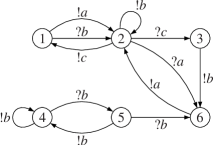
Figure 9: Running example for the proof of Lemma 3.5

For example, given the system depicted in Fig. 9, with $A=\{3\}$ and $B=\{6\}$, one has ${\mathit{Prom}}(A\cup B)=\{1,2,3,4,5,6\}$ and a possible choice for the paths $\pi_{x}$ is given in Fig. 10.

We now define a sequence ${{\mathcal{P}}}_{0},{{\mathcal{P}}}_{1},\ldots$ of partitions of ${\mathit{Prom}}(A\cup B)$. In general ${{\mathcal{P}}}_{k}$ is some $\{B_{1}^{k},B_{2}^{k},\ldots\}$ and each class $B_{j}^{k}\in{{\mathcal{P}}}_{k}$ comes with a fixed element $b_{j}^{k}$ called its representative (which is underlined in the examples). The first partition is composed of all singletons: ${{\mathcal{P}}}_{0}=\{\{x\}\mid x\in{\mathit{Prom}}(A\cup B)\}$. Partition ${{\mathcal{P}}}_{k+1}$ is coarser than ${{\mathcal{P}}}_{k}$: each class in ${{\mathcal{P}}}_{k+1}$ is the fusion of (possibly only one) classes of ${{\mathcal{P}}}_{k}$. Assume ${{\mathcal{P}}}_{k}$ is given: ${{\mathcal{P}}}_{k}=\{B_{1}^{k},\ldots\}$ with $\{b_{1}^{k},\ldots\}$ as representatives. We define a mapping $f_{k+1}$ between the classes of ${{\mathcal{P}}}_{k}$. For any class $B_{j}^{k}$, we consider its representative $b_{j}^{k}$, shortly written $x$, and associate with $B_{j}^{k}$ the class to which $x^{k+1}$ (the $k+1$-th location on $\pi_{x}$) belongs. In our running example $f_{1}$ is given on Fig. 10.

$\pi_{1}$	$\stackrel{{\scriptstyle\mbox{\scriptsize def}}}{{=}}$	$(1,\varepsilon)\to(2,a)\to(6,\varepsilon)$		$f_{1}(\{\underline{1}\})$	$=$	$\{2\}$
$\pi_{2}$	$\stackrel{{\scriptstyle\mbox{\scriptsize def}}}{{=}}$	$(2,\varepsilon)\to(2,b)\to(1,bc)\to(2,c)\to(3,\varepsilon)$		$f_{1}(\{\underline{2}\})$	$=$	$\{2\}$		$f_{4}(\{1,\underline{2}\})$	$=$	$\{3\}$
$\pi_{3}$	$\stackrel{{\scriptstyle\mbox{\scriptsize def}}}{{=}}$	$(3,\varepsilon)$		$f_{1}(\{\underline{3}\})$	$=$	$\{3\}$		$f_{4}(\{\underline{3}\})$	$=$	$\{3\}$
$\pi_{4}$	$\stackrel{{\scriptstyle\mbox{\scriptsize def}}}{{=}}$	$(4,\varepsilon)\to(4,b)\to(4,bb)\to(5,b)\to(6,\varepsilon)$		$f_{1}(\{\underline{4}\})$	$=$	$\{4\}$		$f_{4}(\{\underline{4},5\})$	$=$	$\{6\}$
$\pi_{5}$	$\stackrel{{\scriptstyle\mbox{\scriptsize def}}}{{=}}$	$(5,\varepsilon)\to(4,b)\to(4,bb)\to(5,b)\to(6,\varepsilon)$		$f_{1}(\{\underline{5}\})$	$=$	$\{4\}$
$\pi_{6}$	$\stackrel{{\scriptstyle\mbox{\scriptsize def}}}{{=}}$	$(6,\varepsilon)$		$f_{1}(\{\underline{6}\})$	$=$	$\{6\}$		$f_{4}(\{\underline{6}\})$	$=$	$\{6\}$

Figure 10: Running example (continued): paths $\pi_{x}$ with mappings $f_{1}$ and $f_{4}$

The mapping $f_{k+1}$ induces an oriented graph (of out-degree $1$). The classes of ${{\mathcal{P}}}_{k+1}$ are obtained by fusing the classes of ${{\mathcal{P}}}_{k}$ which belong to the same connected component in this graph.

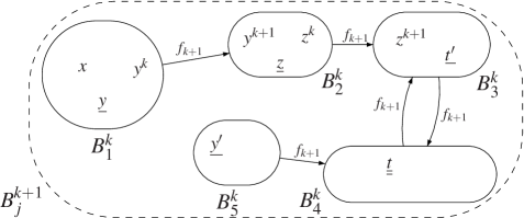
Figure 11: Constructing ${{\mathcal{P}}}_{k+1}$ by fusing equivalence classes from ${{\mathcal{P}}}_{k}$

For example, in Fig. 11, the classes $B_{1}^{k}$, $B_{2}^{k}$, $B_{3}^{k}$, $B_{4}^{k}$ and $B_{5}^{k}$ are fused. The representative for $B^{k+1}_{j}$ is arbitrarily chosen among the representatives of the $B^{k}_{i}$’s that compose the strongly connected component ($b_{3}^{k}$ or $b_{4}^{k}$ in Fig. 11). Back to the running example, we derive ${{\mathcal{P}}}_{1}=\{\{1,\underline{2}\},\{\underline{3}\},\{\underline{4},5\},\{\underline{6}\}\}$ with ${2,3,4,6}$ as representatives (no choice here). Partition ${{\mathcal{P}}}_{1}$ is stable by $f_{2}$ and $f_{3}$.

$$f_{2},f_{3}:\ \{1,\underline{2}\}\to\{1,2\}\ \ \ \ \{\underline{3}\}\to\{3\}\ \ \ \ \{\underline{4},5\}\to\{4,5\}\ \ \ \ \{\underline{6}\}\to\{6\}$$

Hence ${{\mathcal{P}}}_{3}={{\mathcal{P}}}_{2}={{\mathcal{P}}}_{1}$. Mapping $f_{4}$ is given in Fig. 10. We deduce ${{\mathcal{P}}}_{4}=\{\{1,2,\underline{3}\},\{4,5,\underline{6}\}\}$ with $3$ and $6$ as representatives (no choice either).

It is clear that ${{\mathcal{P}}}_{k+1}$ is coarser than ${{\mathcal{P}}}_{k}$ and that a representative at level $k+1$ was already a representative at level $k$. Hence the sequence eventually stabilizes (the state space is finite). We denote ${{\mathcal{P}}}_{\infty}=\{B^{\infty}_{1},\ldots\}$ the partition in the limit. In the running example ${{\mathcal{P}}}_{\infty}={{\mathcal{P}}}_{4}$.

This whole construction is geared towards the following:

Lemma A.1

For all $k\geq 1$, there exists a scheduler ${\mathcal{U}}_{k}$ such that, for every class $B_{j}^{k}$, and writing $y$ for $b_{j}^{k}$,

$$\forall x\in B_{j}^{k}\;\;\forall w\in{{\mathsf{M}}^{*}}^{\mathsf{C}}\;\;\Pr\nolimits_{{\mathcal{U}}_{k}}\bigl{(}(x,w)\models\Diamond(y^{k},w_{y}^{k})\bigr{)}=1$$ (*)

In other words, at step $k$ of the construction there exists a scheduler that, starting from a location $x$ with arbitrary channel content, ensures (with probability one) we’ll visit the $k$-th configuration on $\pi_{y}$ where $y$ is the representative for $x$ in ${{\mathcal{P}}}_{k}$. When $k$ is large enough, more precisely larger than all $|\pi_{x}|$’s, (* ‣ A.1) states that ${\mathcal{U}}_{k}$ guarantees reaching $A$ (or $B$, depending on $x$) with probability one, which concludes the proof of Lemma 3.5.

(of Lemma A.1).

The proof is by induction on $k$.

We first prove the case $k=1$. Let $x$ be a location in some class $B_{i}^{1}$ having $(y=)b_{i}^{1}$ as representative. The behavior of ${\mathcal{U}}_{1}$ is simple: in any configuration $(z,v)$, ${\mathcal{U}}_{1}$ fires $\delta_{z}^{0}$. Going on this way, ${\mathcal{U}}_{1}$ eventually ends up in the strongly connected component (w.r.t $f_{1}$). Because of the finite-attractor property, the configuration $(y,\varepsilon)$ is visited infinitely often almost surely. Hence, ${\mathcal{U}}_{1}$ will succeed in reaching $(y^{1},w_{y}^{1})$ from $(y,\varepsilon)$ by $\delta_{y}^{1}$.

Assume now that for some $k\geq 1$ there exists ${\mathcal{U}}_{k}$ ensuring (* ‣ A.1). We consider ${{\mathcal{P}}}_{k+1}$ and build ${\mathcal{U}}_{k+1}$, using ${\mathcal{U}}_{k}$. Let $x\in B_{j}^{k+1}$ (it may help to look at Fig. 11). Starting from $(x,w)$, ${\mathcal{U}}_{k+1}$ behaves as ${\mathcal{U}}_{k}$ until $(y^{k},w_{y}^{k})$ is reached. Then it fires $\delta_{y}^{k}$ and ends up in $(y^{k+1},w^{\prime})$ for some channel content $w^{\prime}$. $y^{k+1}$ is a location of $B_{i^{\prime}}^{k}=f_{k+1}(B_{i}^{k})$; let $z=b_{i^{\prime}}^{k}$ be its representative. From configuration $(y^{k+1},w^{\prime})$, ${\mathcal{U}}_{k+1}$ behaves again as ${\mathcal{U}}_{k}$ and eventually reaches $(z^{k},w_{z}^{k})$ with probability one. Iterating this process (alternation of ${\mathcal{U}}_{k}$’s behavior and one step transition), ${\mathcal{U}}_{k+1}$ will eventually end in the strongly connected component of $B_{j}^{k+1}$. If $t$ is the representative for this class in ${{\mathcal{P}}}_{k+1}$, because of the finite-attractor property $(t,\varepsilon)$ is visited infinitely often, almost surely. Hence, ${\mathcal{U}}_{k+1}$ will in the end succeed and reach $(t^{k+1},w_{t}^{k+1})$ using ${\mathcal{U}}_{k}$ until $(t^{k},w_{t}^{k})$ and then performing $\delta_{t}^{k}$. ∎

eceived November 2005; accepted March 2006

References

- Abdulla et al. (2005) Abdulla, P. A., Baier, C., Purushothaman Iyer, S., and Jonsson, B. 2005. Simulating perfect channels with probabilistic lossy channels. Information and Computation 197, 1–2, 22–40.
- Abdulla et al. (2005) Abdulla, P. A., Bertrand, N., Rabinovich, A., and Schnoebelen, Ph. 2005. Verification of probabilistic systems with faulty communication. Information and Computation 202, 2, 141–165.
- Abdulla et al. (2000) Abdulla, P. A., čerāns, K., Jonsson, B., and Tsay, Y.-K. 2000. Algorithmic analysis of programs with well quasi-ordered domains. Information and Computation 160, 1/2, 109–127.
- Abdulla et al. (2004) Abdulla, P. A., Collomb-Annichini, A., Bouajjani, A., and Jonsson, B. 2004. Using forward reachability analysis for verification of lossy channel systems. Formal Methods in System Design 25, 1, 39–65.
- Abdulla and Jonsson (1996a) Abdulla, P. A. and Jonsson, B. 1996a. Undecidable verification problems for programs with unreliable channels. Information and Computation 130, 1, 71–90.
- Abdulla and Jonsson (1996b) Abdulla, P. A. and Jonsson, B. 1996b. Verifying programs with unreliable channels. Information and Computation 127, 2, 91–101.
- Baier et al. (2006) Baier, C., Bertrand, N., and Schnoebelen, Ph. 2006. A note on the attractor-property of infinite-state Markov chains. Information Processing Letters 97, 2, 58–63.
- Baier and Engelen (1999) Baier, C. and Engelen, B. 1999. Establishing qualitative properties for probabilistic lossy channel systems: An algorithmic approach. In Proc. 5th Int. AMAST Workshop Formal Methods for Real-Time and Probabilistic Systems (ARTS ’99), Bamberg, Germany, May 1999. Lecture Notes in Computer Science, vol. 1601. Springer, 34–52.
- Bertrand and Schnoebelen (2003) Bertrand, N. and Schnoebelen, Ph. 2003. Model checking lossy channels systems is probably decidable. In Proc. 6th Int. Conf. Foundations of Software Science and Computation Structures (FOSSACS 2003), Warsaw, Poland, Apr. 2003. Lecture Notes in Computer Science, vol. 2620. Springer, 120–135.
- Bertrand and Schnoebelen (2004) Bertrand, N. and Schnoebelen, Ph. 2004. Verifying nondeterministic channel systems with probabilistic message losses. In Proc. 3rd Int. Workshop on Automated Verification of Infinite-State Systems (AVIS 2004), Barcelona, Spain, Apr. 2004, R. Bharadwaj, Ed.
- Brand and Zafiropulo (1983) Brand, D. and Zafiropulo, P. 1983. On communicating finite-state machines. Journal of the ACM 30, 2, 323–342.
- Cécé et al. (1996) Cécé, G., Finkel, A., and Purushothaman Iyer, S. 1996. Unreliable channels are easier to verify than perfect channels. Information and Computation 124, 1, 20–31.
- Courcoubetis and Yannakakis (1995) Courcoubetis, C. and Yannakakis, M. 1995. The complexity of probabilistic verification. Journal of the ACM 42, 4, 857–907.
- Emerson (1990) Emerson, E. A. 1990. Temporal and modal logic. In Handbook of Theoretical Computer Science, J. v. Leeuwen, Ed. Vol. B. Elsevier Science, Chapter 16, 995–1072.
- Finkel (1994) Finkel, A. 1994. Decidability of the termination problem for completely specificied protocols. Distributed Computing 7, 3, 129–135.
- Finkel and Schnoebelen (2001) Finkel, A. and Schnoebelen, Ph. 2001. Well-structured transition systems everywhere! Theoretical Computer Science 256, 1–2, 63–92.
- Grädel et al. (2002) Grädel, E., Thomas, W., and Wilke, T., Eds. 2002. Automata, Logics, and Infinite Games: A Guide to Current Research. Lecture Notes in Computer Science, vol. 2500. Springer.
- Kemeny et al. (1966) Kemeny, J. G., Snell, J. L., and Knapp, A. W. 1966. Denumerable Markov Chains. D. Van Nostrand Co., Princeton, NJ, USA.
- Masson and Schnoebelen (2002) Masson, B. and Schnoebelen, Ph. 2002. On verifying fair lossy channel systems. In Proc. 27th Int. Symp. Math. Found. Comp. Sci. (MFCS 2002), Warsaw, Poland, Aug. 2002. Lecture Notes in Computer Science, vol. 2420. Springer, 543–555.
- Mayr (2003) Mayr, R. 2003. Undecidable problems in unreliable computations. Theoretical Computer Science 297, 1–3, 337–354.
- Pachl (1987) Pachl, J. K. 1987. Protocol description and analysis based on a state transition model with channel expressions. In Proc. 7th IFIP WG6.1 Int. Workshop on Protocol Specification, Testing, and Verification (PSTV ’87), Zurich, Switzerland, May 1987. North-Holland, 207–219.
- Panangaden (2001) Panangaden, P. 2001. Measure and probability for concurrency theorists. Theoretical Computer Science 253, 2, 287–309.
- Purushothaman Iyer and Narasimha (1997) Purushothaman Iyer, S. and Narasimha, M. 1997. Probabilistic lossy channel systems. In Proc. 7th Int. Joint Conf. Theory and Practice of Software Development (TAPSOFT ’97), Lille, France, Apr. 1997. Lecture Notes in Computer Science, vol. 1214. Springer, 667–681.
- Puterman (1994) Puterman, M. L. 1994. Markov decision processes: discrete stochastic dynamic programming. John Wiley & Sons.
- Rabinovich (2003) Rabinovich, A. 2003. Quantitative analysis of probabilistic lossy channel systems. In Proc. 30th Int. Coll. Automata, Languages, and Programming (ICALP 2003), Eindhoven, NL, July 2003. Lecture Notes in Computer Science, vol. 2719. Springer, 1008–1021.
- Schnoebelen (2001) Schnoebelen, Ph. 2001. Bisimulation and other undecidable equivalences for lossy channel systems. In Proc. 4th Int. Symp. Theoretical Aspects of Computer Software (TACS 2001), Sendai, Japan, Oct. 2001. Lecture Notes in Computer Science, vol. 2215. Springer, 385–399.
- Schnoebelen (2002) Schnoebelen, Ph. 2002. Verifying lossy channel systems has nonprimitive recursive complexity. Information Processing Letters 83, 5, 251–261.
- Schnoebelen (2004) Schnoebelen, Ph. 2004. The verification of probabilistic lossy channel systems. In Validation of Stochastic Systems – A Guide to Current Research, C. Baier et al., Eds. Lecture Notes in Computer Science, vol. 2925. Springer, 445–465.
- Vardi (1985) Vardi, M. Y. 1985. Automatic verification of probabilistic concurrent finite-state programs. In Proc. 26th Symp. Foundations of Computer Science (FOCS ’85), Portland, OR, USA, Oct. 1985. IEEE Comp. Soc. Press, 327–338.
- Vardi (1999) Vardi, M. Y. 1999. Probabilistic linear-time model checking: An overview of the automata-theoretic approach. In Proc. 5th Int. AMAST Workshop Formal Methods for Real-Time and Probabilistic Systems (ARTS ’99), Bamberg, Germany, May 1999. Lecture Notes in Computer Science, vol. 1601. Springer, 265–276.