On Interleaving Techniques for MIMO Channels and Limitations of Bit Interleaved Coded Modulation

Abstract

It is shown that while the mutual information curves for coded modulation (CM) and bit interleaved coded modulation (BICM) overlap in the case of a single input single output channel, the same is not true in multiple input multiple output (MIMO) channels. A method for mitigating fading in the presence of multiple transmit antennas, named coordinate interleaving (CI), is presented as a generalization of component interleaving for a single transmit antenna. The extent of any advantages of CI over BICM, relative to CM, is analyzed from a mutual information perspective; the analysis is based on an equivalent parallel channel model for CI. Several expressions for mutual information in the presence of CI and multiple transmit and receive antennas are derived. Results show that CI gives higher mutual information compared to that of BICM if proper signal mappings are used. Effects like constellation rotation in the presence of CI are also considered and illustrated; it is shown that constellation rotation can increase the constrained capacity.

I Introduction

Mitigating the effects of fading on the decoding of forward error correction codes has been studied for single transmit antenna configurations, and revolves around some form of interleaving. Traditionally, interleaving was performed directly on the coded bits present at the encoder’s output. Given that coded modulation (CM) [22] is optimal, the recognition of the fact that modulation and coding are no longer necessarily combined when interleaving an encoder’s output—i.e., prior to mapping the (interleaved) bits to complex (channel) alphabet symbols—has naturally led researchers [13] to study capacity limitations of bit interleaved coded modulation (BICM) schemes; see [13] and references therein for definition of BICM. In the case of single transmit antenna configurations, the conclusion was that mutual information remains essentially the same—provided that Gray mapping is used to map the interleaved coded bits to modulator’s points. This reinforced a potential advantage of BICM, i.e., flexibility from the perspective of adaptive coding and modulation schemes. Other aspects of the study in [13] related to the cut-off rate—but this concept has been deemed irrelevant with the advance of iterative decoding and concatenated coding schemes (e.g., turbo codes). As a result, BICM was deemed desirable, and was employed in standards for CDMA [17] and satellite systems that involve one transmit antenna.

In parallel, an alternative to separating coding from modulation was studied for single transmit antenna configurations, and named coordinate (or component) interleaving [18]. In that approach, the real and imaginary coordinates were interleaved separately, and diversity was derived from the encoder’s trellis (minimum Hamming distance); there was no difficulty reading the interleaved coordinates, because complex symbols were transmitted from only one transmit antenna, and the orthogonal in-phase and quadrature components could be naturally and separately detected. The idea of interleaving the real coordinates, or components, of points from multidimensional constellations embedded in some Cartesian product of the complex field ℂ was discussed in [26]; therein, an algebraic number theoretic analysis was pursued to support the conclusion that coordinate interleaving (CI) together with constellation rotation can increase diversity—separately from any redundancy scheme such as forward error correction coding. The diversity was quantified in terms of a coordinate-wise Hamming distance. In [19] the authors restricted the MIMO channel to a two transmit antenna configuration, and relied on constellation rotation along with an orthogonal space-time diversity scheme [1] to increase diversity by increasing the coordinate-wise Hamming distance; coordinates of a rotated complex constellation were first interleaved then mapped to orthogonal space-time block code matrices for two transmit antennas [1]. By allowing the symbols from the two transmit antennas to be easily separable at the receive antenna due to orthogonality, orthogonal space time block codes allow the approach in [18] to be extended to two transmit antennas.

The problem is more complicated when multiple transmit antennas are employed, as coordinates can no longer be observed independently from each other due to the superposition of all transmitted complex symbols at any receive antenna. A version of BICM for multiple input multiple output (MIMO) channels was examined in [24, 25].

A more general scheme for CI in the presence of multiple transmit antennas was reported in [27], and summarized in Section II below; while the exemplary illustration in [27] was based on a two transmit antenna configuration, it can be applied to any number of transmit antennas. In addition, it can be employed simultaneously with a coding redundancy scheme (concatenated or not), does not require separating coding from modulation, and does not rely on constellation rotation—although rotation is not precluded; it is easily recognized to differ from channel interleaving, which would interleave blocks of (all) complex symbols to be transmitted from all transmit antennas during one MIMO channel use. This CI scheme offers a means to mitigate diversity in MIMO channels, which generalizes the single antenna concept in a non-obvious manner. The minimum coordinate-wise Hamming distance can be naturally controlled in the design of the forward error correcting scheme; in essence, after coding and modulation (possibly combined) the real and imaginary coordinates from the complex symbols of all transmit antennas are interleaved over an arbitrary block length, e.g. a frame, and then transmitted as new coordinates in the respective MIMO configuration. Further considerations may be possible using the algebraic number theoretic formalism undertaken in [26]. Depending on the original complex constellation(s) used on the transmit antennas, the complex channel alphabet after CI may change over the wireless channel. Moreover, the coordinate interleaver can be viewed as an interleaver in a serially concatenated scheme, thus enabling iterations between decoding and detection in a manner similar to turbo decoding; this is also described in a separate work [27]. This paper is not concerned with the details of combining coding redundancy and CI, the latter briefly reviewed in Section II; rather, the impact of CI on diversity, via the minimum coordinate-wise Hamming distance, motivates one to investigate mutual information limits. This is the main purpose of this manuscript, which sets out to determine the extent of any advantages of CI over BICM, relative to CM, from a mutual information perspective. It should be noted that in this paper we are dealing with capacity limits for finite alphabet constellations (constrained constellations)—rather than the generally used ergodic capacity, which is often associated with the case of continuous alphabets.

Section II reviews the mechanism by which CI affects diversity in a MIMO system. Section III examines the mutual information with finite size alphabets in the single transmit antenna case [13], as well as in several MIMO configurations; the numerical results illustrate that the fact that mutual information curves for CM and BICM overlap in the case of a single transmit antenna ought not to be taken for granted, as a significant gap occurs in MIMO channels. Section IV introduces an equivalent parallel channel model for CI, and derives several expressions for mutual information in the presence of CI and multiple transmit antennas. Section V-B examines effects like constellation rotation in the presence of CI. Conclusions are drawn in Section VI.

II Coordinate Interleaving for MIMO Channels – Diversity Perspective

Consider a MIMO scenario where the number of transmit and, respectively, receive antennas are $N$ and $M$. Let the complex symbols transmitted from the $N$ transmit antennas during $l$ uses of the MIMO channel be represented as a long vector, whose entries are superscripted by the transmit antenna index, and subscripted by the channel use index. Conditioned on knowledge of the channel state information (CSI), the probability of transmitting

$$e =$$ [e_0^(1)e_0^(2)…e_0^(N)e_1^(1)…e_1^(N)…e_l-1^(1)…e_l-1^(N)]^T (2)

and deciding in favor of

$$c =$$ [c_0^(1)c_0^(2)…c_0^(N)c_1^(1)…c_1^(N)…c_l-1^(1)…c_l-1^(N)]^T (4)

at the maximum likelihood decoder is bounded as below

$$\mbox{Pr}\{\mbox{\boldmath$c$}\!\mapsto\!\mbox{\boldmath$e$}|\alpha_{ij}[k],i=1,\ldots,N,j=1,\ldots,M,k=0,\ldots,l-1\}\\ \leq\exp(-d^{2}_{E}(\mbox{\boldmath$e$},\mbox{\boldmath$c$})E_{s}/4N_{0}),$$

where $\alpha_{i,j}(\cdot)$ are the channel coefficients between transmit antenna $i$ and receive antenna $j$, with $E\{|\alpha_{i,j}|^{2}\}=1$, $\forall i,j$. The key parameter is clearly

$$d^{2}_{E}(\mbox{\boldmath$e$},\mbox{\boldmath$c$})=\sum_{j=1}^{M}\sum_{k=0}^{l-1}\left|\sum_{i=1}^{N}\alpha_{i,j}[k](c_{k}^{(i)}-e_{k}^{(i)})\right|^{2}.$$ (5)

As is well-known [2]

$$d^{2}_{E}(\mbox{\boldmath$e$},\mbox{\boldmath$c$})=\sum_{j=1}^{M}\sum_{k=0}^{l-1}\mbox{\boldmath$\Omega$}_{j}[k]\mbox{\boldmath$C$}[k]\mbox{\boldmath$\Omega$}_{j}^{\dagger}[k],$$ (6)

where

$$\mbox{\boldmath$\Omega$}_{j}[k]=\left[\alpha_{1,j}[k],\ldots,\alpha_{N,j}[k]\right],$$ (7)

$$\mbox{\boldmath$C$}[k]=(\mbox{\boldmath$c$}_{k}-\mbox{\boldmath$e$}_{k})(\mbox{\boldmath$c$}_{k}-\mbox{\boldmath$e$}_{k})^{\dagger}=\left[\begin{array}[]{@{\,}c}c_{k}^{(1)}-e_{k}^{(1)}\\ c_{k}^{(2)}-e_{k}^{(2)}\\ \vdots\\ c_{k}^{(N)}-e_{k}^{(N)}\end{array}\right]\left[\left(c_{k}^{(1)}-e_{k}^{(1)}\right)^{*},\ldots,\left(c_{k}^{(N)}-e_{k}^{(N)}\right)^{*}\right],$$ (8)

where the superscript $\ast$ indicates complex conjugation. Since $\mbox{\boldmath$C$}[k]$ is Hermitian, it admits the singular value decomposition (SVD)

$$\mbox{\boldmath$C$}[k]=\mbox{\boldmath$V$}[k]\mbox{\boldmath$D$}[k]\mbox{\boldmath$V$}^{\rm H}[k]$$ (9)

where the superscript ‘H’ indicates a Hermitian operation (complex conjugated transposition). Denote by $D_{ii}[k]$, $1\leq i\leq N$, the diagonal elements of $\mbox{\boldmath$D$}[k]$, which is diagonal per SVD transform. The vector $\mbox{\boldmath$\Omega$}_{j}[k]$ of relevant channel coefficients (to receive antenna $j$) is transformed by virtue of the SVD into

$$\left[\beta_{1,j}[k],\ldots,\beta_{N,j}[k]\right]=\mbox{\boldmath$\Omega$}_{j}[k]\mbox{\boldmath$V$}[k].$$ (10)

Because $\mbox{\boldmath$V$}[k]$ is unitary, the independent complex Gaussian random variables (r.v.s) $\alpha_{1,j}[k],\ldots,\alpha_{N,j}[k]$ are transformed into a new set of $N$ i.i.d. r.v.s. In other words, there exists an equivalent set of channels $\beta_{1,j}[k],\ldots,\beta_{N,j}[k]$ that characterizes the transmission. Therefore, for each channel use $k$, and each receive antenna $j$,

$$\mbox{\boldmath$\Omega$}_{j}[k]\mbox{\boldmath$C$}[k]\mbox{\boldmath$\Omega$}_{j}^{\dagger}[k]=\sum_{i=1}^{N}\left|\beta_{i,j}[k]\right|^{2}D_{ii}[k].$$ (11)

By definition, $\mbox{\boldmath$C$}[k]$ has rank 1 (that is, if the set $\begin{array}[]{@{\,}c@{\,}c@{\,}c@{\,}c@{\,}}c_{k}^{(1)}&c_{k}^{(2)}&\ldots&c_{k}^{(N)}\end{array}$ is different from $\begin{array}[]{@{\,}c@{\,}c@{\,}c@{\,}c@{\,}}e_{k}^{(1)}&e_{k}^{(2)}&\ldots&e_{k}^{(N)}\end{array}$); thereby, exactly one value among $D_{11}[k]\ldots D_{NN}[k]$, be it $D_{i_{0}i_{0}}[k]$, is nonzero. The nonzero value must necessarily equal the trace of $\mbox{\boldmath$C$}[k]$, which in turn equals obviously

$$\mbox{tr}\mbox{\boldmath$C$}[k]=\sum_{i=1}^{N}|c_{k}^{(i)}-e_{k}^{(i)}|^{2}=\|\mbox{\boldmath$c$}_{k}-\mbox{\boldmath$e$}_{k}\|^{2}.$$ (12)

Consequently, the key parameter $d_{E}^{2}(\mbox{\boldmath$e$},\mbox{\boldmath$c$})$ reduces to

$$\mbox{\boldmath$\Omega$}_{j}[k]\mbox{\boldmath$C$}[k]\mbox{\boldmath$\Omega$}_{j}^{\dagger}[k]=\left|\beta_{i_{0},j}[k]\right|^{2}D_{i_{0}i_{0}}[k]=\left|\beta_{i_{0},j}[k]\right|^{2}\cdot\sum_{i=1}^{N}|c_{k}^{(i)}-e_{k}^{(i)}|^{2}.$$ (13)

Clearly, there exists an equivalent set of independent complex Gaussian channels derived from the original set of independent complex Gaussian channels, and exactly one of them affects all of the coordinates of the multidimensional point $\begin{array}[]{@{\,}c@{\,}c@{\,}c@{\,}c@{\,}}(c_{k}^{(1)}&c_{k}^{(2)}&\ldots&c_{k}^{(N)})\end{array}$ transmitted during channel use $k$; this means that if the nonzero equivalent channel $\beta_{i_{0},j}[k]$ fades, it will affect all $2N$ coordinates transmitted during the $k$th channel use. The essence of CI is summarized by

Theorem 1

There exists an equivalent set of independent complex Gaussian channels derived from $\alpha_{1j}[k]\!,\!\ldots\!,\!\alpha_{Nj}[k]$, such that exactly one of them affects all (real/imaginary) coordinates of a transmitted multidimensional point $(c_{k}^{(1)},\ldots,c_{k}^{(N)})\in\!\!\mbox{\hollow R}^{2N}$, via $\mbox{\boldmath$\Omega$}_{j}[t]\mbox{\boldmath$C$}[t]\mbox{\boldmath$\Omega$}_{j}^{\dagger}[t]\!=\!|\beta_{i_{0},j}(t)|^{2}\sum_{i=1}^{N}\!\!\left[\left(c_{t,{\rm I}}^{(i)}-e_{t,{\rm I}}^{(i)}\right)^{2}\!\!+\!\left(c_{t,{\rm Q}}^{(i)}-e_{t,{\rm Q}}^{(i)}\right)^{2}\right]$.

Theorem 1 implies that, when using multiple transmit antennas and CM possibly over non-binary fields, with or without puncturing, it is desirable to:

1. Interleave the coordinates of transmitted multidimensional constellation points in order to enable, and render meaningful, a Hamming distance with respect to coordinates—rather than complex symbols; and,

2. Design codes for multiple transmit antennas that can maximize the minimum coordinate-wise (as opposed to complex-symbol-wise per current state of the art [2]) Hamming distance between codewords, in order to derive the most diversity from CI

Note that, in general, CI is different from BICM [13] (see also Example 1), and does not preclude (or destroy) the concept of CM (via signal-space coding); this is so because CI operates on the (real-valued) coordinates of the complex values from the complex modulator alphabet, rather than operating on the coded bits, prior to the modulator [13, Fig. 1].

It is possible to design space-time codes for CI that exhibit diversity exceeding that of existing codes; this, however, is the scope of a separate work [27]. The sequel is concerned with characterizing CI from a mutual information perspective.

III Mutual information limits for CM and BICM: Is BICM Efficient in MIMO Channels?

If the model in [13] is used to characterize mutual information limits for CM and BICM schemes that involve $N>1$ transmit antennas (only scenario $N=1$ was discussed in [13]) the curves in Fig. 1 are obtained; the numerical results were computed by an extension to MIMO channels of the analysis (and numerical approach) from [13]. The curves in Fig. 1 indicate a fundamental difference between the information rate limits in scenarios that involve finite channel alphabets, and more than one transmit/receive antennas—even for the Gray mapping case, which in [13] is conjectured to maximize the mutual information of bit-interleaved schemes. (It is possible to view CM as a concatenation between a code and a mapper, provided that the mapper is derived from some set partitioning labelling.) While it can be rigorously proven that CI does not change the ergodic channel capacity, the model in [13] predicts a gap between mutual information curves for BICM relative to pure CM (due, in part, to the finite size channel alphabet; see, however, the footnote in [13, p. 931]). The relevant mutual information curves are illustrated in Fig. 1; with $N=2$ transmit antennas and $M=1$ receive antenna, the gap is significant, but narrows when $M=2$.

Note that in CI schemes the role of iterating between decoding and detection is to circumvent maximum likelihood detection; the presence of an interleaver does not always preclude maximum likelihood—e.g., a symbol interleaver in a CM scheme does not. It should be noted that if iterative demodulation and decoding is used for CI (same as for BICM), it is possible to approach the i.i.d. CM capacity limit, since iterations improve the quality of the soft information being exchanged between the demodulator and decoder. However, this paper attempts to quantify only the case of non-iterative demodulation/decoding.

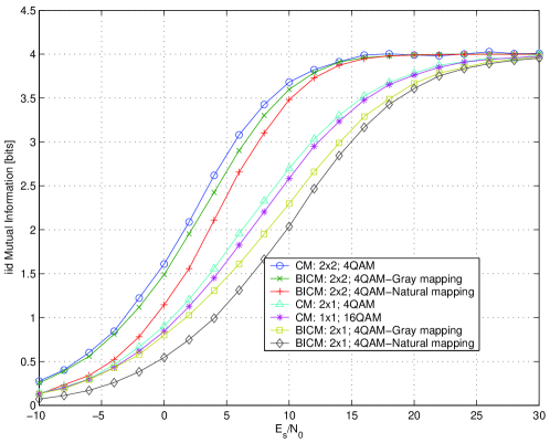
Figure 1: Mutual information for CM vs. BICM [13], with finite 4PSK modulation alphabets, two transmit antennas and either 1 or 2 receive antennas, and memoryless fading channels. The mutual information for CM was computed based on the model and approach from [13], using the computational tool described in [14], based on the BCJR algorithm.

To further illustrate the undesirable effect of BICM, Fig. 2 shows the relevant mutual information curves when $N=M=2$, and 16QAM is used on the individual transmit antennas.

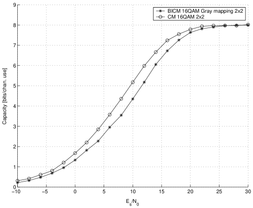
Figure 2: Mutual information for CM vs. BICM [13], with finite 16QAM modulation alphabets, two transmit antennas and 2 receive antennas, in memoryless fading channels; note increased gap. The mutual information for CM was computed based on the model and approach from [13], using the computational tool described in [14], based on the BCJR algorithm.

From the above 2 figures, we see that BICM suffers a big loss in mutual information compared to CM in MIMO channels. This, together with the diversity advantage of CI shown in the previous section motivate us to investigate the CI in a mutual information perspective. Results will show that CI outperforms BICM in terms of mutual information and narrows the gap relative to CM. The following section is a derivation of mutual information for a CI scheme in MIMO channels.

IV Mutual Information for Coordinate Interleaved Schemes in MIMO Rayleigh Fading Channels

As a result of coding and modulation, $2N$ (in-phase and quadrature) coordinates are generated during any channel use for transmission from the $N$ transmit antennas; coordinates are collected from all MIMO channel uses (over a long enough frame), and interleaved in such a manner as to insure that any $2N$ coordinates—which, in the absence of CI, would be transmitted from the $N$ transmit antennas during the same MIMO channel use—are transmitted (as in-phase and quadrature components) from different antennas, during different MIMO channel uses; i.e., each of the $2N$ coordinates will experience independent fading relative to each other [but the same fading as some other $2N-1$ coordinates along with which it is eventually transmitted during some channel use, per eq.  (13)]. Specifically, let the number of MIMO channel uses in one coordinate interleaved frame be $l$; the coordinate interleaver size is then $2Nl$. Denote by $\mbox{\boldmath$x$}_{k^{\prime}}$ the $2N$ dimensional symbol formed by the $2N$ coordinates that are to be transmitted, post CI, from the $N$ transmit antennas during the $k^{\prime}$-th MIMO channel use, $k^{\prime}=0,\ldots,l-1$:

$$\textstyle{\mbox{\boldmath$x$}_{k^{\prime}}\in{\cal X}\stackrel{{\scriptstyle\mbox{\scriptsize def}}}{{=}}\{\mbox{\boldmath$x$}|\mbox{\boldmath$x$}=[x_{0},\ldots,x_{2N-1}]^{\rm T}\sim[x(1)\ldots x(N)]^{\rm T}\},}$$ (14)

where $\sim$ denotes a known isomorphism between real and complex vectors, and

$$x(m+1)=x_{2m}j+x_{2m+1}\in{\cal M},\ \ m=0,\ldots,N-1,$$ (15)

is a complex symbol, from some constellation $\cal M$ (see below), to be sent from the $(m+1)$-st transmit antenna; the constellation $\cal M$ will arise as the Cartesian product of the in-phase and quadrature alphabets post CI. (The resulting constellation mapping after CI, $\cal M$, will be the same with the original mapping for square QAM modulation; and different for general PSK modulation.) Further, denote by $\{c_{k}\}_{0}^{2Nl-1}$, respectively $\{\kappa_{k}\}_{0}^{2Nl-1}$, the coordinates before and after interleaving. A coordinate $2N$-tuple $\{\kappa_{k}\}_{2Np}^{2Np+2N-1}$, $p\in{\mbox{\hollow N}}$, will be said to form an $N$-antenna label, because they would all form the $2N$ coordinates to be sent from the $N$ antennas during the same channel use; more specifically, the coordinates whose index is congruent modulo 2 with 0, respectively 1, will form the quadrature and in-phase components.

In order to model the CI operation, let $c_{k}$ be permuted to $\kappa_{\pi_{0}(k)2N+\pi_{1}(k)}$, i.e., the coordinate interleaver permutation will be $\pi:k\mapsto\left(\pi_{0}(k),\pi_{1}(k)\right)$, $\pi_{1}(k)=0,1,\ldots,2N-1$, $\pi_{0}(k)=0,1,\ldots,l-1$. That is, $c_{k}$ is transmitted during the $\pi_{0}(k)$-th MIMO channel use, as the $\pi_{1}(k)$-th component of the $N$-antenna label of $\mbox{\boldmath$x$}_{k^{\prime}}|_{k^{\prime}=\pi_{0}(k)}$. The receiver has to detect the $i$-th component of $\mbox{\boldmath$x$}_{k^{\prime}}$ and unpermute it to obtain $c_{\pi^{-1}(k^{\prime},i)}$. Note that the component pairs $x_{2m},x_{2m+1}$ are affected by the same fade, namely the channel fading coefficient on the link between transmit antenna $m+1$ and the relevant receive antenna.

As long as the coordinate interleaver has sufficient depth (to insure exposure to independent fades), the index $\pi_{0}(k)$ of the MIMO channel use that conveys, after interleaving, a (pre-interleaving) coordinate $c_{k}$ becomes irrelevant from the perspective of computing the mutual information; further, coordinate $c_{k}$ appears as a random element $\pi_{1}(k)$ of some $N$-antenna label (a $2N$-dimensional point), whose components are detected individually—after having been affected by a common fading coefficient (see eq.  (13)). The random position in an $N$-antenna label can be modeled by a switch $S_{\ell}$, and the equivalent parallel model is shown in Fig. 3.

Figure 3: Equivalent parallel channel model for computing mutual information in the presence of CI—assuming ideal (coordinate) interleaving, $N$ transmit antennas; depicted channel conveys one $q_{\cup}$-ary r.v., carried in a random position of an $N$-antenna label. The total mutual information with CI will be $2N$ times the capacity of this channel; $y_{s,i}$ is the observation of the $i$-th channel at the $s$-th receive antenna. $h(l)$ represents the channel coefficient from the $l$-th transmit antenna to the $s$-th receive antenna; $x(l)$ is the complex value, from some complex alphabet $\cal M$, transmitted from the $l$-th transmit antenna. The complex constellation $\cal M$ arises as the Cartesian product of the quadrature and in-phase alphabets post component interleaving; $q_{\cup}$ is the cardinality of both the in-phase and the quadrature alphabets post component interleaving—each coordinate alphabet being, in turn, the union of the in-phase and quadrature alphabets prior to component interleaving.

The complex constellation $\cal M$ mentioned above arises as the Cartesian product of the quadrature and in-phase alphabets post component interleaving; in order to further define the formalism, assume for simplicity that prior to CI the modulator employs the same complex constellation $\cal Q$ on each of the $N$ transmit antennas. Let ${\cal Q}_{I}$ and ${\cal Q}_{Q}$ be, respectively, the alphabets pertaining to the in-phase and quadrature coordinates of points from $\cal Q$ prior to CI. Since CI mixes the in-phase and quadrature coordinates, each coordinate post interleaving will belong to an alphabet $Q_{\cup}$ that is the union of the alphabets ${\cal Q}_{I}$ and ${\cal Q}_{Q}$, ${\cal Q}_{\cup}\stackrel{{\scriptstyle\mbox{\scriptsize def}}}{{=}}{\cal Q}_{I}\cup{\cal Q}_{Q}$. Therefore, let

$$q_{\cup}\stackrel{{\scriptstyle\mbox{\scriptsize def}}}{{=}}|{\cal Q}_{\cup}|=|{\cal Q}_{I}\cup{\cal Q}_{Q}|$$ (16)

be the cardinality of both the in-phase and the quadrature alphabets post component interleaving—each coordinate alphabet being, in turn, the union of the in-phase and quadrature alphabets prior to component interleaving. Then the effective (post-interleaving) complex constellation associated with any transmit antenna becomes

$${\cal M}=({\cal Q}_{I}\cup{\cal Q}_{Q})\times({\cal Q}_{I}\cup{\cal Q}_{Q}),$$ (17)

and the MIMO constellation post CI, $\cal X$, is the $N$-fold Cartesian product of $\cal M$ with itself,

$${\cal X}={\cal M}^{N}.$$ (18)

Finally, the operation of mapping real (post-interleaving) coordinates $\kappa_{k}$ to multidimensional points is defined naturally, in that a coordinate $\kappa_{k}$ simply becomes a component of some multidimensional point $\mbox{\boldmath$x$}\in{\cal X}$, and its label; unlike in BICM [13], where Gray mapping has been conjectured to be optimal, the mapping of coordinates to $N$-antenna labels is unambiguous (no multiple choices).

The problem then becomes calculating the mutual information between pre-interleaving $2N$-tuples $\left[c_{0},c_{1},\ldots,c_{2N-1}\right]^{\rm T}$ and the receiver observations at the $2N$ different MIMO channel uses that convey, post component interleaving, those coordinates; clearly this model involves buffering. If CI is such as to insure that each uninterleaved coordinate is sent during independent MIMO channel uses, than the desired mutual information is $2N$ times the mutual information of an abstract channel conveying a single, $q_{\cup}$-ary, post-interleaving coordinate, i.e. between an interleaved coordinate and the observations—by the $M$ receive antennas—of the multidimensional point from ${\cal M}^{N}$ that carries the corresponding interleaved coordinate. The assumption of ideal interleaving reduces, thereby, the relevant problem to the random switch model in Fig. 3. The auxiliary switch $S_{\ell}$ will be eliminated by averaging over its possible realizations from $\{0,\ldots,2N-1\}$; this will require one to compute the mutual information of the $i$-th channel, i.e. between $\kappa_{i}$ and $\mbox{\boldmath$y$}_{i}=[y_{1,i}\ldots y_{M,i}]^{\rm T}$ in Fig. 3, where $y_{s,i}$ is the complex observation by receive antenna $s$ of the output of the $i$-th channel, $i$ is a realization of the r.v.  $S_{\ell}$, and the $\kappa_{i}$-s are i.i.d.. Therefore, the effect of CI is modeled by the operation of the switch $S_{\ell}$, and by the assumption of independence between MIMO channel uses.

Example 1

By visual inspection, one easily and rigorously verifies that when $\cal Q$ is an unrotated 4QAM constellation, ${\cal Q}_{I}={\cal Q}_{Q}={\cal Q}_{\cup}$, ${\cal M}={\cal Q}$, $q_{\cup}=2$—i.e. the inputs to the parallel channels in Fig. 3 are binary r.v.s, like in BICM; on another hand the BICM channel input is an $m$-tuple with $m=N\log_{2}|{\cal Q}|=2N$. Thereby, Fig. 3 reduces to the equivalent BICM model from [13, Fig. 3] that corresponds to using a 4QAM constellation on each transmit antenna (although [13] restricts itself to a single transmit antenna, the BICM model from [13] is directly generalized to $N>1$ with the additional averaging in the form of marginal probabilities, as discussed in Section IV-B). Consequently, BICM and CI are equivalent in the 4PSK case, for any number of transmit antennas $N$. This proves in part (i.e. for the 4PSK scenario) Biglieri et al.’s conjecture made in [13] that Gray mapping is optimal for BICM. $\diamondsuit$

In the context defined above, the sequel addresses the scenario when the receiver has perfect or partial channel state information, or no channel state information—and, of course, the information necessary to unpermute the coordinates; the latter translates in information about the switch $S_{\ell}$. In general, as it will turn out below, computing the desired mutual information in the presence or absence of channel state information reduces to computing $I(\kappa;\mbox{\boldmath$y$},\mbox{\boldmath$\theta$},\mbox{$S_{\ell}$}=i)$ or $I(\kappa;\mbox{\boldmath$y$},\mbox{$S_{\ell}$}=i)$, where $\theta$ represents a (generalized) channel state parameter, i.e. a vector parameter on which the transition between channel input and output depends. The mutual information $I(\kappa;\mbox{\boldmath$y$},\mbox{\boldmath$\theta$},\mbox{$S_{\ell}$}=i)$ will be derived below in order to reveal the computational approach for numerically computing it; the modifications necessary to obtain $I(\kappa;\mbox{\boldmath$y$},\mbox{$S_{\ell}$}=i)$ will be straightforward.

IV-A Problem setting and notations

Lower case symbols will denote scalar quantities (real or complex), boldface symbols will denote vectors, and underlined boldface symbols will denote sequences of scalars or of vectors.

In general, the channel input at channel use $k$, denoted generically $\mbox{\boldmath$x$}_{k}$, can be viewed as a point (vector) from some real $N_{1}$ dimensional space ${\mbox{\hollow R}}^{N_{1}}$—or, for even $N_{1}\geq 2$, from a complex $N_{1}/2$ dimensional space ${\mbox{\hollow C}}^{N_{1}/2}$; the complex vector entries can be further limited to some complex (i.e., real two dimensional) alphabet $\cal Q$, in which case the overall complex $N_{1}/2$ dimensional alphabet, denoted $\cal X$, has finite cardinality $|{\cal X}|\stackrel{{\scriptstyle\mbox{\scriptsize def}}}{{=}}M_{0}$, often verifying $M_{0}=2^{m}$. In the case of CM for MIMO channels the channel input relevant to computing the mutual information is a complex $N$ dimensional point (vector), whereby $N_{1}=2N$—see [13], albeit [13] only addressed the single antenna scenario $N=M=1$); for BICM the relevant channel input is a bit $m$-tuple [13], i.e. a point from ${\mbox{\hollow R}}^{m}$, and a parallel channel model [13, Fig. 3] reduces it to a single bit, i.e. a point from $\{0,1\}\in{\mbox{\hollow R}}$, whereby $N_{1}=1$. In the CI case, the relevant channel input is a point in ${\mbox{\hollow R}}^{2N}$, and the parallel channel model from Fig. 3 reduces it to a single dimensional real point from ${\cal Q}_{\cup}\stackrel{{\scriptstyle\mbox{\scriptsize def}}}{{=}}{\cal Q}_{I}\cup{\cal Q}_{Q}$.

The output $y$ of the channel, generally from some ${\mbox{\hollow C}}^{N_{2}}$ space, can be viewed for the MIMO problem at hand as a point (vector) from a complex $M$ dimensional space, with $M$ being the number of receive antennas, whereby $N_{2}=M$; this is true both for the aggregate MIMO channel and for any one of the parallel channels in Fig. 3.

In order to correctly identify the state vector as a point from some complex space ${\mbox{\hollow C}}^{N^{\prime}}$, consider the $i$-th parallel channel in Fig. 3, and note that the channel output is a collection of $M$ receive antenna observables; even when the channel from any transmit antenna to any receive antenna is memoryless, the observable at receive antenna $s$ depends not only on the current channel coefficients and on coordinate $\kappa_{i}$ (during the current MIMO channel use), but also on the remaining coordinates—other than $\kappa_{i}$—arriving at the receive antenna $s$ on the other channels during the current MIMO channel use, and acting as interference. Thereby the state vector for the $i$-th subchannel is

$$\mbox{\boldmath$\theta$}_{i}=\left[h_{1,1},\ldots,h_{1,M},\ldots,h_{N,1},\ldots,h_{N,M},\kappa_{0},\ldots,\kappa_{i-1},\right.$$ (19)

$$\left.\kappa_{i+1},\ldots,\kappa_{2N-1}\right]^{\rm T}\!=\!\left[\mbox{\boldmath$\theta$}_{\rm Ch}^{\rm T},\mbox{\boldmath$\theta$}_{{\rm MI},i}^{\rm T}\right]^{\rm T}\!\!\!\in{\cal C}^{NM+2N-1},$$

whereby $N^{\prime}\stackrel{{\scriptstyle\mbox{\scriptsize def}}}{{=}}NM+2N-1$, and where $h_{l,s}\in{\mbox{\hollow C}}$ are complex Gaussian r.v.s of unit variance and zero mean, modeling independent flat fading coefficients from transmit antenna $l$ to receive antenna $s$.

Thereby, when transmitting (and detecting!) a $q_{\cup}$-ary r.v.  $\kappa$ on a random position $i$ in an $N$-antenna label (see Fig. 3), the channel state can be viewed as a random parameter with (random) realizations $\mbox{\boldmath$\theta$}_{i}$ that depend on the realizations of $S_{\ell}$.

IV-B Coherent vs. non-coherent detection—$p_{\mbox{\boldmath$\theta$}}(\mbox{\boldmath$y$}|\mbox{\boldmath$x$})$ vs. $p(\mbox{\boldmath$y$}|\mbox{\boldmath$x$})$

The important implication of the above form of the state vector is that even when the receiver knows the MIMO channel perfectly, lack of information about any interfering coordinates renders the problem noncoherent (partial channel information, or no channel state information). The following discussion serves to meaningfully characterize the differences between coherent, noncoherent, and partially coherent scenarios.

The assumption of coherence vs. noncoherence essentially translates in whether the relevant pdf is conditioned on the channel state, or averaged over the channel state. One characteristic of the MIMO channel is that the part of the channel state vector that depends of the multiple transmit antenna interference is always unknown (except possibly when talking about pilot symbols), and therefore the detection is always at least partially non-coherent; it will be necessary to average the pdf over the unknown part of the channel (even when the actual fading coefficients are known to the receiver), and this task will be naturally achieved by computing marginal probabilities. Note that the non-coherent aspect is responsible for the gap between CM and BICM in MIMO channels. Formally, this can be briefly described as follows.

In the coherent case the channel is characterized by the family of transition probability density functions

$$\left\{p_{\mbox{\boldmath$\theta$}}(\mbox{\boldmath$y$}|\mbox{\boldmath$x$})\left|\mbox{\boldmath$\theta$}\in{\mbox{\hollow C}}^{N^{\prime}},\mbox{\boldmath$x$}\in{\mbox{\hollow R}}^{N_{1}},\mbox{\boldmath$y$}\in{\mbox{\hollow C}}^{N_{2}}\right.\right\}$$ (20)

where the vector parameter $\theta$ represents the channel state. The sequence of channel state vectors from a set of channel uses is denoted $\underline{\mbox{\boldmath$\theta$}}$. The essential assumption is that $\theta$ is independent of the channel input $x$; e.g., in any of the parallel channels in Fig. 3 $\mbox{\boldmath$\theta$}_{{\rm MI},i}$ does not depend on $\kappa_{i}$—clearly $\mbox{\boldmath$\theta$}_{\rm Ch}$ is independent of $\kappa_{i}$, which makes $\mbox{\boldmath$\theta$}_{i}$ independent of $\kappa_{i}$. In addition it is assumed that, conditioned on $\underline{\mbox{\boldmath$\theta$}}$, the channel is memoryless, i.e.

$$p_{\underline{\mbox{\boldmath$\theta$}}}(\underline{\mbox{\boldmath$y$}}\left|\underline{\mbox{\boldmath$x$}}\right.)=\prod_{k}p_{\mbox{\boldmath$\theta$}_{k}}(\mbox{\boldmath$y$}_{k}\left|\mbox{\boldmath$x$}_{k}\right.).$$ (21)

Note that in ISI channels the state $\theta$ depends on the input sequence, and therefore, given $\underline{\mbox{\boldmath$\theta$}}$, $\underline{\mbox{\boldmath$y$}}$ does depend on the input sequence (i.e. $\mbox{\boldmath$y$}_{k}$ depends not only on $\mbox{\boldmath$x$}_{k}$ but also on $\mbox{\boldmath$x$}_{k-1}$, etc.). Moreover, $\underline{\mbox{\boldmath$\theta$}}$ is assumed to be stationary and have finite memory. OFDM systems do verify the above assumptions, as the channel experienced by the encoder is flat (albeit correlated).

In the general noncoherent case lack of knowledge about $\underline{\mbox{\boldmath$\theta$}}$ prevents the channel transitions from being memoryless. Nevertheless, under ideal interleaving, and for all finite index sets wherein interleaving renders the channel realizations independent, $E_{\underline{\mbox{\boldmath$\theta$}}}\{p_{\underline{\mbox{\boldmath$\theta$}}}(\underline{\mbox{\boldmath$y$}}\left|\underline{\mbox{\boldmath$x$}}\right.)\}=E_{\underline{\mbox{\boldmath$\theta$}}}\{\prod_{k\in{\cal K}}p_{\mbox{\boldmath$\theta$}_{k}}(\mbox{\boldmath$y$}_{k}\left|\mbox{\boldmath$x$}_{k}\right.)\}$ via (21); because of the independence between the elements of the sequence $\underline{\mbox{\boldmath$\theta$}}$ the average of the product equals the product of averages, and one can define

$$p(\mbox{\boldmath$y$}|\mbox{\boldmath$x$})\stackrel{{\scriptstyle\mbox{\scriptsize def}}}{{=}}E_{\underline{\mbox{\boldmath$\theta$}}}\{p_{\underline{\mbox{\boldmath$\theta$}}}(\underline{\mbox{\boldmath$y$}}\left|\underline{\mbox{\boldmath$x$}}\right.)\}=\prod_{k\in{\cal K}}p(\mbox{\boldmath$y$}_{k}\left|\mbox{\boldmath$x$}_{k}\right.)$$

where a new average transition pdf is defined as

$$p(\mbox{\boldmath$y$}\left|\mbox{\boldmath$x$}\right.)=E_{\mbox{\boldmath$\theta$}}\{p_{\mbox{\boldmath$\theta$}}(\mbox{\boldmath$y$}\left|\mbox{\boldmath$x$}\right.)\}.$$ (22)

Using $p(\mbox{\boldmath$y$}\left|\mbox{\boldmath$x$}\right.)$ instead of $p_{\mbox{\boldmath$\theta$}}(\mbox{\boldmath$y$}\left|\mbox{\boldmath$x$}\right.)$ will allow transforming metrics, decision rules, and expressions for average mutual information in the coherent case into same for noncoherent scenarios.

Finally, when relying on the model in Fig. 3, the multiple input part of the state vector $\mbox{\boldmath$\theta$}_{{\rm MI},i}$ will be unknown even when $\mbox{\boldmath$\theta$}_{{\rm Ch},i}$ is known; averaging it out to obtain $p_{\mbox{\boldmath$\theta$}_{{\rm Ch},i}}(\mbox{\boldmath$y$}\left|\mbox{\boldmath$x$}\right.)$ simply means computing marginal probabilities for the coordinate of interest $\kappa_{i}$. This will be used in Section IV-C, and in producing the numerical results.

IV-C Derivation of mutual information for CI

In order to compute the mutual information when transmitting a $q_{\cup}$-ary r.v.  on a random position in an $N$-antenna label, consider a $q_{\cup}$-ary r.v. $\kappa$; the r.v.  $S_{\ell}$, whose outcome determines the switch position, is uniformly distributed over $\{0,\ldots,2N-1\}$, and has known realizations $\mbox{$S_{\ell}$}=i$. For the coherent case, where $\theta$ and the permutation pattern (i.e. $S_{\ell}$) are perfectly known to the receiver, one must calculate the average mutual information $\overline{I(\kappa;\mbox{\boldmath$y$},\mbox{\boldmath$\theta$},\mbox{$S_{\ell}$})}$ as an average of $I(\kappa;\mbox{\boldmath$y$},\mbox{\boldmath$\theta$},\mbox{$S_{\ell}$})$ over $S_{\ell}$, i.e.

$$\overline{I(\kappa;\mbox{\boldmath$y$},\mbox{\boldmath$\theta$},\mbox{$S_{\ell}$})}=\frac{1}{2N}\sum_{i=0}^{2N-1}I(\kappa;\mbox{\boldmath$y$},\mbox{\boldmath$\theta$}_{i},\mbox{$S_{\ell}$}=i);$$ (23)

as noted, the channel state can be viewed as a known random parameter with (random) realizations $\mbox{\boldmath$\theta$}_{i}$; likewise, $S_{\ell}$ is a known random parameter. Similarly, in the noncoherent case, one must compute the average mutual information $\overline{I(\kappa;\mbox{\boldmath$y$},\mbox{$S_{\ell}$})}$ as an average of $I(\kappa;\mbox{\boldmath$y$},\mbox{$S_{\ell}$})$ over $S_{\ell}$, i.e.

$$\overline{I(\kappa;\mbox{\boldmath$y$},\mbox{$S_{\ell}$})}=\frac{1}{2N}\sum_{i=0}^{2N-1}I(\kappa;\mbox{\boldmath$y$},\mbox{$S_{\ell}$}=i);$$ (24)

and, in the partially coherent case—when $\mbox{\boldmath$\theta$}_{\rm Ch}$ is known but the multiple input component of the state vector $\mbox{\boldmath$\theta$}_{\rm MI}$ is unknown—the mutual information is $\overline{I(\kappa;\mbox{\boldmath$y$},\mbox{\boldmath$\theta$}_{\rm Ch},\mbox{$S_{\ell}$})}$ and must be computed as an average of $I(\kappa;\mbox{\boldmath$y$},\mbox{\boldmath$\theta$}_{\rm Ch},\mbox{$S_{\ell}$})$ over $S_{\ell}$, i.e.

$$\overline{I(\kappa;\mbox{\boldmath$y$},\mbox{\boldmath$\theta$}_{\rm Ch},\mbox{$S_{\ell}$})}=\frac{1}{2N}\sum_{i=0}^{2N-1}I(\kappa;\mbox{\boldmath$y$},\mbox{\boldmath$\theta$}_{\rm Ch},\mbox{$S_{\ell}$}=i).$$ (25)

The third case is more physically meaningful than the first (which assumes that the receiver always knows the symbols transmitted from the competing transmit antennas); it is the third mutual information that will be numerically computed in the sequel.

Denoting by $\mbox{\boldmath$\kappa$}\stackrel{{\scriptstyle\mbox{\scriptsize def}}}{{=}}[\kappa_{0},\ldots,\kappa_{2N-1}]^{\rm T}$ the complete MIMO channel input, the desired mutual information expressions in the above scenarios are

$$\overline{I(\mbox{\boldmath$\kappa$};\mbox{\boldmath$y$},\mbox{\boldmath$\theta$},\mbox{$S_{\ell}$})}=2N\overline{I(\kappa;\mbox{\boldmath$y$},\mbox{\boldmath$\theta$},\mbox{$S_{\ell}$})},$$ (26)

$$\overline{I(\mbox{\boldmath$\kappa$};\mbox{\boldmath$y$},\mbox{$S_{\ell}$})}=2N\overline{I(\kappa;\mbox{\boldmath$y$},\mbox{$S_{\ell}$})},$$ (27)

$$\overline{I(\mbox{\boldmath$\kappa$};\mbox{\boldmath$y$},\mbox{\boldmath$\theta$}_{\rm Ch},\mbox{$S_{\ell}$})}=2N\overline{I(\kappa;\mbox{\boldmath$y$},\mbox{\boldmath$\theta$}_{\rm Ch},\mbox{$S_{\ell}$})}.$$ (28)

In the sequel the subscript $i$ of $\mbox{\boldmath$\theta$}_{i}$ will be omitted for simplicity, but is to be understood in the theoretical, perfectly coherent case.

Consider first the coherent case, which requires computing $I(\kappa;\mbox{\boldmath$y$},\mbox{\boldmath$\theta$},\mbox{$S_{\ell}$}=i)$ via (23). By the chain rule for mutual information, $I(\kappa;\mbox{\boldmath$y$},\mbox{\boldmath$\theta$},\mbox{$S_{\ell}$}=i)=I(\kappa;\mbox{$S_{\ell}$}=i)+I(\kappa;\mbox{\boldmath$y$},\mbox{\boldmath$\theta$}|\mbox{$S_{\ell}$}=i)\stackrel{{\scriptstyle\mbox{\scriptsize(a)}}}{{=}}I(\kappa;\mbox{\boldmath$\theta$}|\mbox{$S_{\ell}$}=i)+I(\kappa;\mbox{\boldmath$y$}|\mbox{\boldmath$\theta$},\mbox{$S_{\ell}$}=i)\stackrel{{\scriptstyle\mbox{\scriptsize(b)}}}{{=}}I(\kappa;\mbox{\boldmath$y$}|\mbox{\boldmath$\theta$},\mbox{$S_{\ell}$}=i)$; (a) follows because $I(\kappa;\mbox{$S_{\ell}$}=i)=0$ due to the independence between $\kappa$ and $\mbox{$S_{\ell}$}=i$, and similarly (b). It suffices then to average over the conditional pdf $p(\kappa,\mbox{\boldmath$y$},\mbox{\boldmath$\theta$}|\mbox{$S_{\ell}$}=i)$, and—since $I(\kappa;\mbox{\boldmath$y$},\mbox{\boldmath$\theta$}|\mbox{$S_{\ell}$}=i)=I(\kappa;\mbox{\boldmath$y$}|\mbox{\boldmath$\theta$},\mbox{$S_{\ell}$}=i)$—the conditional mutual information of $\kappa$, $y$, given $\theta$ and $\mbox{$S_{\ell}$}=i$, for the case when $\kappa$ is uniformly distributed in ${\cal Q}_{\cup}$, reduces to (see Appendix A)

$$I(\kappa;\mbox{\boldmath$y$}|\mbox{\boldmath$\theta$},\mbox{$S_{\ell}$}=i)=\log_{2}(q_{\cup})-E_{\kappa,\mbox{\boldmath$y$},\mbox{\boldmath$\theta$}}\left[\log_{2}\frac{\sum_{\mbox{\boldmath$z$}\in{\cal X}}p_{\mbox{\boldmath$\theta$}}(\mbox{\boldmath$y$}|\mbox{\boldmath$z$})}{\sum_{\mbox{\boldmath$\zeta$}\in{\cal X}_{\kappa}^{i}}p_{\mbox{\boldmath$\theta$}}(\mbox{\boldmath$y$}|\mbox{\boldmath$\zeta$})}\right]$$ (29)

where $\kappa$, $y$, and $\theta$ are conditionally distributed as (see Appendix B)

$$p(\kappa,\mbox{\boldmath$y$},\mbox{\boldmath$\theta$}|\mbox{$S_{\ell}$}=i)=q_{\cup}^{-2N}p(\mbox{\boldmath$\theta$})\sum_{\mbox{\boldmath$\zeta$}\in{\cal X}_{\kappa}^{i}}p_{\mbox{\boldmath$\theta$}}(\mbox{\boldmath$y$}|\mbox{\boldmath$\zeta$}).$$ (30)

Above, ${\cal X}_{\kappa}^{i}$ denotes the set of all $N$-antenna labels having $\kappa$ on position $i$, $i=0,\ldots,2N-1$. Finally, using eqs. (23), (26), one obtains the mutual information with CI in the coherent scenario, for the case when $\kappa$ is uniformly distributed in ${\cal Q}_{\cup}$, to be

$$\overline{I(\mbox{\boldmath$\kappa$};\mbox{\boldmath$y$},\mbox{\boldmath$\theta$},\mbox{$S_{\ell}$})}=2N\log_{2}(q_{\cup})-\sum_{i=0}^{2N-1}E_{\kappa,\mbox{\boldmath$y$},\mbox{\boldmath$\theta$}}\left[\log_{2}\frac{\sum_{\mbox{\boldmath$z$}\in{\cal X}}p_{\mbox{\boldmath$\theta$}}(\mbox{\boldmath$y$}|\mbox{\boldmath$z$})}{\sum_{\mbox{\boldmath$\zeta$}\in{\cal X}_{\kappa}^{i}}p_{\mbox{\boldmath$\theta$}}(\mbox{\boldmath$y$}|\mbox{\boldmath$\zeta$})}\right].$$ (31)

Likewise, in the case when $\kappa$ is non-uniformly distributed in ${\cal Q}_{\cup}$,

$$I(\kappa;\mbox{\boldmath$y$}|\mbox{\boldmath$\theta$},\mbox{$S_{\ell}$}=i)=-E_{\kappa,\mbox{\boldmath$y$},\mbox{\boldmath$\theta$}}\left[\log_{2}\frac{\sum_{\mbox{\boldmath$z$}\in{\cal X}}p_{\mbox{\boldmath$\theta$}}(\mbox{\boldmath$y$}|\mbox{\boldmath$z$})p(\mbox{\boldmath$z$})}{\sum_{\mbox{\boldmath$\zeta$}\in{\cal X}_{\kappa}^{i}}p_{\mbox{\boldmath$\theta$}}(\mbox{\boldmath$y$}|\mbox{\boldmath$\zeta$})p(\mbox{\boldmath$\zeta$})}\right],$$ (32)

$$p(\kappa,\mbox{\boldmath$y$},\mbox{\boldmath$\theta$}|\mbox{$S_{\ell}$}=i)=p(\kappa)p(\mbox{\boldmath$\theta$})\sum_{\mbox{\boldmath$\zeta$}\in{\cal X}_{\kappa}^{i}}p_{\mbox{\boldmath$\theta$}}(\mbox{\boldmath$y$}|\mbox{\boldmath$\zeta$})p(\mbox{\boldmath$\zeta$}).$$ (33)

$$\overline{I(\mbox{\boldmath$\kappa$};\mbox{\boldmath$y$},\mbox{\boldmath$\theta$},\mbox{$S_{\ell}$})}=-\sum_{i=0}^{2N-1}E_{\kappa,\mbox{\boldmath$y$},\mbox{\boldmath$\theta$}}\left[\log_{2}\frac{\sum_{\mbox{\boldmath$z$}\in{\cal X}}p_{\mbox{\boldmath$\theta$}}(\mbox{\boldmath$y$}|\mbox{\boldmath$z$})p(\mbox{\boldmath$z$})}{\sum_{\mbox{\boldmath$\zeta$}\in{\cal X}_{\kappa}^{i}}p_{\mbox{\boldmath$\theta$}}(\mbox{\boldmath$y$}|\mbox{\boldmath$\zeta$})p(\mbox{\boldmath$\zeta$})}\right].$$ (34)

Similarly in the noncoherent case, when $\kappa$ is uniformly distributed in ${\cal Q}_{\cup}$,

$$\overline{I(\mbox{\boldmath$\kappa$},\mbox{\boldmath$y$},\mbox{$S_{\ell}$})}=2N\log_{2}(q_{\cup})-\sum_{i=0}^{2N-1}E_{\kappa,\mbox{\boldmath$y$}}\left[\log_{2}\frac{\sum_{\mbox{\boldmath$z$}\in{\cal X}}p(\mbox{\boldmath$y$}|\mbox{\boldmath$z$})}{\sum_{\mbox{\boldmath$\zeta$}\in{\cal X}_{\kappa}^{i}}p(\mbox{\boldmath$y$}|\mbox{\boldmath$\zeta$})}\right],$$ (35)

where $p(\mbox{\boldmath$y$}|\mbox{\boldmath$z$})$ is obtained as in Section IV-B; and in the partial coherent case, when the fading coefficients are known to the receiver,

$$\overline{I(\mbox{\boldmath$\kappa$};\mbox{\boldmath$y$},\mbox{\boldmath$\theta$}_{\rm Ch},\mbox{$S_{\ell}$})}=2N\log_{2}(q_{\cup})-\sum_{i=0}^{2N-1}E_{\kappa,\mbox{\boldmath$y$},\mbox{\boldmath$\theta$}_{\rm Ch}}\left[\log_{2}\frac{\sum_{\mbox{\boldmath$z$}\in{\cal X}}p_{\mbox{\boldmath$\theta$}_{\rm Ch}}(\mbox{\boldmath$y$}|\mbox{\boldmath$z$})}{\sum_{\mbox{\boldmath$\zeta$}\in{\cal X}_{\kappa}^{i}}p_{\mbox{\boldmath$\theta$}_{\rm Ch}}(\mbox{\boldmath$y$}|\mbox{\boldmath$\zeta$})}\right],$$ (36)

where averaging over the multiple input component of the channel state vector, per (22), is implemented naturally via marginal probabilities.

Similar expressions can be derived in the noncoherent and partially coherent scenarios for the case when $\kappa$ is non-uniformly distributed in ${\cal Q}_{\cup}$; in the latter case

$$\overline{I(\mbox{\boldmath$\kappa$};\mbox{\boldmath$y$},\mbox{\boldmath$\theta$}_{\rm Ch},\mbox{$S_{\ell}$})}=-\sum_{i=0}^{2N-1}E_{\kappa,\mbox{\boldmath$y$},\mbox{\boldmath$\theta$}_{\rm Ch}}\left[\log_{2}\frac{\sum_{\mbox{\boldmath$z$}\in{\cal X}}p_{\mbox{\boldmath$\theta$}_{\rm Ch}}(\mbox{\boldmath$y$}|\mbox{\boldmath$z$})p(\mbox{\boldmath$z$})}{\sum_{\mbox{\boldmath$\zeta$}\in{\cal X}_{\kappa}^{i}}p_{\mbox{\boldmath$\theta$}_{\rm Ch}}(\mbox{\boldmath$y$}|\mbox{\boldmath$\zeta$})p(\mbox{\boldmath$\zeta$})}\right],$$ (37)

V Numerical results

For a variety of MIMO configurations and constellation sizes the mutual information in the presence of CI is shown in Figs. 4–7, along with mutual information for BICM and CM. While the fading coefficients are assumed known to the receiver, the interfering symbols transmitted from other antennas are not known, and are averaged out as discussed in Section IV-B (essentially computing marginal likelihood probabilities); mathematically, the figures plot $\overline{I}(\mbox{\boldmath$\kappa$};\mbox{\boldmath$y$},\mbox{\boldmath$\theta$}_{\rm Ch})$.

V-A Complex constellations that are invariant to CI

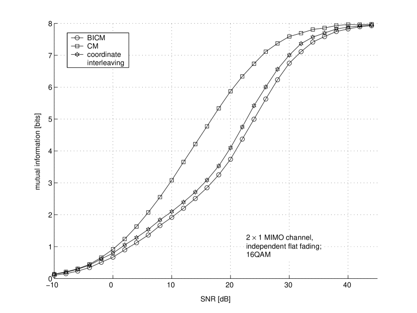
Figure 4: Mutual information comparison between BICM (with pure Gray mapping) and CM with and without CI, in a Rayleigh fading MIMO configuration with two transmit and one receive antennas, and 16QAM constellations.

Complex constellations like 4PSK, 16QAM, 64QAM are invariant to CI; i.e., all possible combinations of valid coordinates of either type (real or imaginary) result in valid constellation points. Mathematically this means that ${\cal Q}=({\cal Q}_{I}\cup{\cal Q}_{Q})\times({\cal Q}_{I}\cup{\cal Q}_{Q})$, as opposed to ${\cal Q}\subset({\cal Q}_{I}\cup{\cal Q}_{Q})\times({\cal Q}_{I}\cup{\cal Q}_{Q})$. One can easily visualize this, and such cases are illustrated in Figs. 4, 5, 6; Fig. 7 includes two single transmit antenna scenarios for comparison.

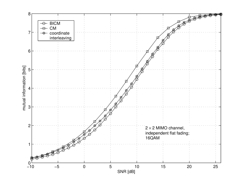
Figure 5: Mutual information comparison between BICM (with pure Gray mapping) and CM with and without CI, in a Rayleigh fading MIMO configuration with two transmit and receive antennas, and 16QAM constellations.

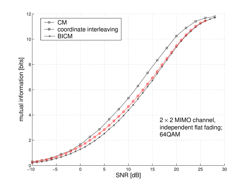
Figure 6: Mutual information comparison between BICM (with pure Gray mapping) and CM with and without CI, in a Rayleigh fading MIMO configuration with two transmit and receive antennas, and 64QAM constellations.

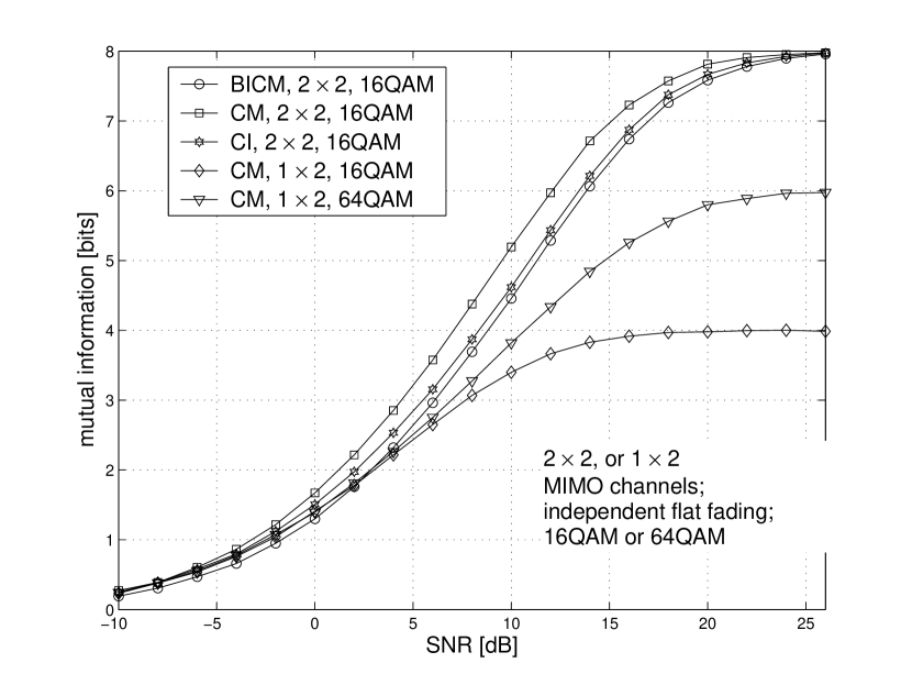
Figure 7: Mutual information comparison between BICM (with pure Gray mapping) and CM with and without CI, in a Rayleigh fading MIMO configuration with either one or two transmit, and receive antennas, and 16QAM, 64QAM constellations. Interestingly, while the $2\times 2$ BICM curve crosses below the $1\times 2$ curves at low SNR, the $2\times 2$ CI curve is always above the $1\times 2$ curves.

V-B Complex constellations that grow in size after CI

An example of complex constellation that is not invariant with respect to CI is the cross-shaped 32QAM. This constellation does not admit a pure Gray mapping, but there exists an optimum impure Gray coding [23] with a Gray penalty of 7/6 (this should be as close to 1 as possible; pure Gray mapping corresponds to Gray penalty of 1). More importantly, ${\cal Q}\subset({\cal Q}_{I}\cup{\cal Q}_{Q})\times({\cal Q}_{I}\cup{\cal Q}_{Q})$, and thereby putting together arbitrary coordinates—which are otherwise valid—results in points that are not necessarily present in the original constellation; the richer constellation can send more bits per channel use asymptotically with SNR, which means that the mutual information curve in the presence of CI can cross even the CM curve at high mutual information values; see Fig. (8). The implication is that it is possible to alleviate the capacity limit by CI, at high information levels.

It is possible to evaluate exactly the upper mutual information margin for a given, finite, constellation size; the simple observation is that for any two r.v.s $X,Y$

$$I(X;Y)=H(X)-H(X|Y);$$

note that, asymptotically with SNR—i.e., as the noise becomes negligible—$Y$ resembles $X$ more and more, and replicates $X$ in the limit. Thereby, as ${\rm SNR}\rightarrow\infty$, $H(X|Y)\rightarrow H(X|X)=0$ and $I(X;Y)\rightarrow H(X)$; this was to be expected, since the maximum mutual information cannot exceed the source’s entropy. In this context $X$ will be a r.v. with realizations in $\cal M$ from (17). A cross shaped 32QAM constellation $\cal Q$, when used on each transmit antenna prior to CI, gives rise to a thirty six point constellation $\cal M$ after CI (replicated $N$ times to form $\cal X$ when $N$ transmit antennas are used). In the enhanced constellation $\cal M$ there are four points that occur with probability of $1/64$, sixteen points with probability of $3/128$, and sixteen points with probability of $9/256$. The set of probabilities of complex $N$-tuples corresponding to the $N$ transmit antennas is the $N$ fold Cartesian product of this set of probabilities with itself; alternatively, the entropy of the $N$ antenna labels is $N$ times the entropy corresponding to one antenna (antenna streams are assumed independent). It can be easily verified that for the thirty six point enhanced constellation the entropy equals $5.12$ bits, which after multiplication by $N=2$ yields more than the $10$ bit information limit that bounds both CM and BICM using the original cross shaped 32QAM constellation; this is indeed consistent with Figs. 8, 9, and explains the cross over between CM and CI.

A more pronounced constellation enhancement effect can be obtained by constellation rotation; the extent of constellation enrichment after CI will be more dramatic than in the cross-shaped 32QAM case. Rotated constellations may possess an advantage when CI is used, and may thereby be desirable, because CI results in an enriched effective constellation; grouping scrambled coordinates results in complex values that do not necessarily belong to the original constellation, and the richer, effective channel alphabet leads to higher mutual information (asymptotically with SNR, see Fig. 8), and even crosses above the CM curve in the range of interest. Fig. 8 is a very limited illustration because constellation enrichment was achieved simply due to the inherent structure of the cross-shaped 32QAM constellation (increase was marginal, from 32 to 36 points). Deliberate rotations will increase the constellation size to larger extents, and probably cause the CI curve to cross the CM curve earlier. Fig. 10 shows the effect of rotating a 4PSK constellation by an angle that makes the enhanced constellation be a scaled version of a 16QAM constellation. It might be possible to engage (activate) CI selectively, at hight SNR, in order to increase the throughput while delaying increasing the constellation size.

This aspect deserves further consideration.

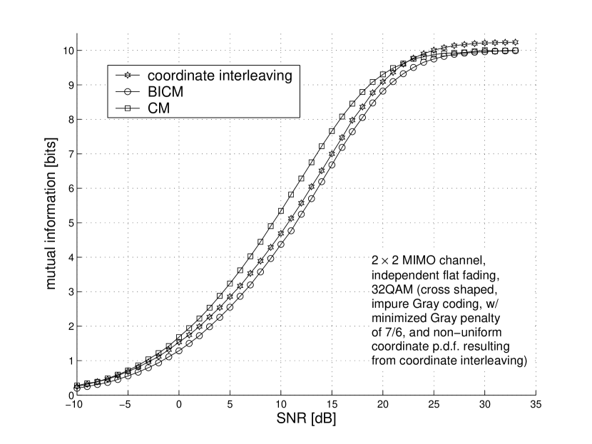
Figure 8: Mutual information comparison between BICM and CM with and without CI, in a Rayleigh fading MIMO configuration with two transmit and receive antennas, and 32QAM constellations.

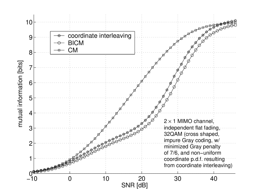
Figure 9: Mutual information comparison between BICM and CM with and without CI, in a Rayleigh fading MIMO configuration with two transmit and one receive antennas, and 32QAM constellations.

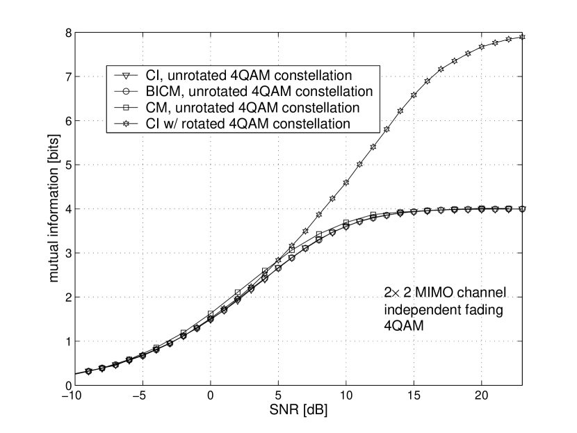
Figure 10: Mutual information comparison between BICM and CM with and without CI, in a Rayleigh fading MIMO configuration with two transmit and receive antennas, using a 4QAM constellation with and without rotation.

Figure 11: When rotated by $\phi=\pi/4-\arctan(1/3)$ and coordinate interleaved, a 4PSK constellation $\{\pm 1\pm j\}$ gives rise to a 16QAM constellation scaled by $\sqrt{2}\sin\left(\arctan(1/3)\right)$.

VI Conclusions

This paper identifies a shortcoming of bit interleaved coded modulation in MIMO fading channels, in terms of constrained i.i.d. mutual information relative to coded modulation; while the mutual information curves for coded modulation and bit interleaved coded modulation overlap in the case of a single input single output channel, a loss in mutual information was observed for bit interleaved coded modulation in MIMO channels. An alternative to bit interleaved coded modulation in MIMO channels, namely coordinate interleaving, was proposed and analyzed. Coordinate interleaving offers better diversity, and improves constrained mutual information over the bit interleaved coded modulation. Effects like constellation rotation and non-uniform constellation points in the presence of CI are also studied.

Appendix A

The derivation of (29) is as follows. First, note that referring to a $q_{\cup}$-ary r.v.  while conditioning on $\mbox{$S_{\ell}$}=i$ is equivalent to referring to $\kappa_{i}$. By definition, if the realizations of a r.v.  $A$ are from $\cal A$, with cardinality $|{\cal A}|$, then the mutual information between r.v.s $A,B$ is

$$I(A;B)=E_{A,B}\left[\log_{2}\frac{p(a,b)}{p(a)p(b)}\right]$$ (38)

$$=-E_{A,B}\left[\log_{2}\frac{p(b)}{p(b|a)}\right]$$

$$=-E_{p(a,b)}\left[\log_{2}\frac{\sum_{\alpha\in{\cal A}}p(b|\alpha)p(\alpha)}{p(b|a)}\right]$$

If $A$ is uniformly distributed in $\cal A$ then $p(\alpha)=|{\cal A}|^{-1},\forall\alpha\in{\cal A}$, which yields

$$I(A;B)=-\log_{2}|{\cal A}|^{-1}-E_{p(a,b)}\left[\log_{2}\frac{\sum_{\alpha\in{\cal A}}p(b|\alpha)}{p(b|a)}\right],$$ (39)

Similarly, if the realizations of a r.v.  $A$ are uniformly distributed in $\cal A$, with $|{\cal A}|=2^{m}$, then the conditional mutual information between r.v.s $A,B$, conditioned on $C$ is $I(A;B|C)=$ $-\log_{2}|{\cal A}|^{-1}-E_{A,B,C}\left[\log_{2}\frac{\sum_{\alpha\in{\cal A}}p(b|\alpha,c)}{p(b|a,c)}\right]$ $=-\log_{2}|{\cal A}|^{-1}-E_{A,B,C}\left[\log_{2}\frac{\sum_{a\in{\cal A}}p_{c}(b|a)}{p_{c}(b|a)}\right],$ where conditioning on $c$ has been represented by writing $c$ as a subscript. Then, in the case when $\kappa$ is uniformly distributed in ${\cal Q}_{\cup}$,

$$I(\kappa;\mbox{\boldmath$y$}|\mbox{\boldmath$\theta$},\mbox{$S_{\ell}$}=i)=\log_{2}(q_{\cup})-E_{\kappa,\mbox{\boldmath$y$},\mbox{\boldmath$\theta$}}\left[\log_{2}\frac{\sum_{a\in{\cal Q}_{\cup}}p_{\mbox{\boldmath$\theta$}}(\mbox{\boldmath$y$}|\kappa=a,\mbox{$S_{\ell}$}=i)}{p_{\mbox{\boldmath$\theta$}}(\mbox{\boldmath$y$}|\kappa,\mbox{$S_{\ell}$}=i)}\right].$$ (40)

But by denoting $\mbox{\boldmath$\kappa$}_{\overline{i}}\stackrel{{\scriptstyle\mbox{\scriptsize def}}}{{=}}\{\kappa_{0},\ldots,\kappa_{i-1},\kappa_{i+1},\ldots,\kappa_{2N-1}\}$ one can write

$$p_{\mbox{\boldmath$\theta$}}(\mbox{\boldmath$y$}|\kappa,\mbox{$S_{\ell}$}=i)=p_{\mbox{\boldmath$\theta$}}(\mbox{\boldmath$y$}|\kappa_{i}=\kappa)$$

$$=\sum_{\mbox{\boldmath$\kappa$}_{\overline{i}}}p_{\mbox{\boldmath$\theta$}}\left(\mbox{\boldmath$y$},\mbox{\boldmath$\kappa$}_{\overline{i}}\ \ |\kappa_{i}=\kappa\right)$$

$$=\sum_{\mbox{\boldmath$\kappa$}_{\overline{i}}}p_{\mbox{\boldmath$\theta$}}\left(\mbox{\boldmath$y$}|\ \ \kappa_{i}=\kappa,\mbox{\boldmath$\kappa$}_{\overline{i}}\right)q_{\cup}^{-(2N-1)}$$

$$=q_{\cup}^{-(2N-1)}\sum_{\mbox{\boldmath$\zeta$}\in{\cal X}_{\kappa}^{i}}p_{\mbox{\boldmath$\theta$}}(\mbox{\boldmath$y$}|\mbox{\boldmath$\zeta$}),$$

and

$$\sum_{a\in{\cal Q}_{\cup}}p_{\mbox{\boldmath$\theta$}}(\mbox{\boldmath$y$}|\kappa=a,\mbox{$S_{\ell}$}=i)$$

$$=\sum_{a\in{\cal Q}_{\cup}}p_{\mbox{\boldmath$\theta$}}(\mbox{\boldmath$y$}|\kappa_{i}=a)$$

$$=\sum_{a\in{\cal Q}_{\cup}}\sum_{\mbox{\boldmath$\kappa$}_{\overline{i}}}p_{\mbox{\boldmath$\theta$}}\left(\mbox{\boldmath$y$},\mbox{\boldmath$\kappa$}_{\overline{i}}\ \ |\kappa_{i}=a\right)$$

$$=\sum_{a\in{\cal Q}_{\cup}}\sum_{\mbox{\boldmath$\kappa$}_{\overline{i}}}p_{\mbox{\boldmath$\theta$}}\left(\mbox{\boldmath$y$}|\ \ \kappa_{i}=a,\mbox{\boldmath$\kappa$}_{\overline{i}}\right)q_{\cup}^{-(2N-1)}$$

$$=q_{\cup}^{-(2N-1)}\sum_{\mbox{\boldmath$z$}\in{\cal X}}p_{\mbox{\boldmath$\theta$}}(\mbox{\boldmath$y$}|\mbox{\boldmath$z$}),$$

hence (29) follows after simplifying $q_{\cup}^{-(2N-1)}$. Likewise, in the case when $\kappa$ is non-uniformly distributed in ${\cal Q}_{\cup}$,

$$I(\kappa;\mbox{\boldmath$y$}|\mbox{\boldmath$\theta$},\mbox{$S_{\ell}$}=i)=-E_{\kappa,\mbox{\boldmath$y$},\mbox{\boldmath$\theta$}}\left[\log_{2}\frac{\sum_{a\in{\cal Q}_{\cup}}p_{\mbox{\boldmath$\theta$}}(\mbox{\boldmath$y$}|\kappa=a,\mbox{$S_{\ell}$}=i)p(a)}{p_{\mbox{\boldmath$\theta$}}(\mbox{\boldmath$y$}|\kappa,\mbox{$S_{\ell}$}=i)}\right]$$ (41)

By denoting $\mbox{\boldmath$\kappa$}_{\overline{i}}\stackrel{{\scriptstyle\mbox{\scriptsize def}}}{{=}}\{\kappa_{0},\ldots,\kappa_{i-1},\kappa_{i+1},\ldots,\kappa_{2N-1}\}$ one can write

$$p_{\mbox{\boldmath$\theta$}}(\mbox{\boldmath$y$}|\kappa,\mbox{$S_{\ell}$}=i)p(\kappa)=p_{\mbox{\boldmath$\theta$}}(\mbox{\boldmath$y$}|\kappa_{i}=\kappa)$$

$$=\sum_{\mbox{\boldmath$\kappa$}_{\overline{i}}}p_{\mbox{\boldmath$\theta$}}\left(\mbox{\boldmath$y$},\mbox{\boldmath$\kappa$}_{\overline{i}}\ \ |\kappa_{i}=\kappa\right)$$

$$=\sum_{\mbox{\boldmath$\kappa$}_{\overline{i}}}p_{\mbox{\boldmath$\theta$}}\left(\mbox{\boldmath$y$}|\ \ \kappa_{i}=\kappa,\mbox{\boldmath$\kappa$}_{\overline{i}}\right)p(\mbox{\boldmath$\kappa$}_{\overline{i}})$$

$$=\sum_{\mbox{\boldmath$\zeta$}\in{\cal X}_{\kappa}^{i}}p_{\mbox{\boldmath$\theta$}}(\mbox{\boldmath$y$}|\mbox{\boldmath$\zeta$})p(\mbox{\boldmath$\zeta$}),$$

and

$$\sum_{a\in{\cal Q}_{\cup}}p_{\mbox{\boldmath$\theta$}}(\mbox{\boldmath$y$}|\kappa=a,\mbox{$S_{\ell}$}=i)p(a)$$

$$=\sum_{a\in{\cal Q}_{\cup}}p_{\mbox{\boldmath$\theta$}}(\mbox{\boldmath$y$}|\kappa_{i}=a)p(a)$$

$$=\sum_{a\in{\cal Q}_{\cup}}\sum_{\mbox{\boldmath$\kappa$}_{\overline{i}}}p_{\mbox{\boldmath$\theta$}}\left(\mbox{\boldmath$y$},\mbox{\boldmath$\kappa$}_{\overline{i}}\ \ |\kappa_{i}=a\right)p(a)$$

$$=\sum_{a\in{\cal Q}_{\cup}}\sum_{\mbox{\boldmath$\kappa$}_{\overline{i}}}p_{\mbox{\boldmath$\theta$}}\left(\mbox{\boldmath$y$}|\ \ \kappa_{i}=a,\mbox{\boldmath$\kappa$}_{\overline{i}}\right)p(\mbox{\boldmath$\kappa$}_{\overline{i}})p(a)$$

$$=\sum_{\mbox{\boldmath$z$}\in{\cal X}}p_{\mbox{\boldmath$\theta$}}(\mbox{\boldmath$y$}|\mbox{\boldmath$z$})p({\mbox{\boldmath$z$}}),$$

hence (32) follows.

Appendix B

The derivation of (30) is as follows. Note that $\kappa,\mbox{\boldmath$\theta$}$ do not depend on $S_{\ell}$; then

$$p(\kappa,\mbox{\boldmath$y$},\mbox{\boldmath$\theta$}|\mbox{$S_{\ell}$}=i)=p(\mbox{\boldmath$y$}|\kappa,\mbox{\boldmath$\theta$},\mbox{$S_{\ell}$}=i)p(\kappa,\mbox{\boldmath$\theta$}|\mbox{$S_{\ell}$}=i)$$

$$=p_{\mbox{\boldmath$\theta$}}(\mbox{\boldmath$y$}|\kappa_{i}=\kappa)p(\kappa,\mbox{\boldmath$\theta$}|\mbox{$S_{\ell}$}=i)$$

$$=p_{\mbox{\boldmath$\theta$}}(\mbox{\boldmath$y$}|\kappa_{i}=\kappa)p(\kappa)p(\mbox{\boldmath$\theta$})$$

$$=q_{\cup}^{-1}p(\mbox{\boldmath$\theta$})\sum_{\mbox{\boldmath$\kappa$}_{\overline{i}}}p_{\mbox{\boldmath$\theta$}}(\mbox{\boldmath$y$},\mbox{\boldmath$\kappa$}_{\overline{i}}|\kappa_{i}=\kappa)$$

$$=q_{\cup}^{-1}p(\mbox{\boldmath$\theta$})\sum_{\mbox{\boldmath$\kappa$}_{\overline{i}}}p_{\mbox{\boldmath$\theta$}}(\mbox{\boldmath$y$}|\mbox{\boldmath$\kappa$}_{\overline{i}},\kappa_{i}=\kappa)q_{\cup}^{-(2N-1)}$$

$$=q_{\cup}^{-2N}p(\mbox{\boldmath$\theta$})\sum_{\mbox{\boldmath$\zeta$}\in{\cal X}_{\kappa}^{i}}p_{\mbox{\boldmath$\theta$}}(\mbox{\boldmath$y$}|\mbox{\boldmath$\zeta$}).$$

Finally, when $\kappa$ is non-uniformly distributed in ${\cal Q}_{\cup}$, (33) is proved via

$$p(\kappa,\mbox{\boldmath$y$},\mbox{\boldmath$\theta$}|\mbox{$S_{\ell}$}=i)=p(\mbox{\boldmath$y$}|\kappa,\mbox{\boldmath$\theta$},\mbox{$S_{\ell}$}=i)p(\kappa,\mbox{\boldmath$\theta$}|\mbox{$S_{\ell}$}=i)$$

$$=p_{\mbox{\boldmath$\theta$}}(\mbox{\boldmath$y$}|\kappa_{i}=\kappa)p(\kappa,\mbox{\boldmath$\theta$}|\mbox{$S_{\ell}$}=i)$$

$$=p_{\mbox{\boldmath$\theta$}}(\mbox{\boldmath$y$}|\kappa_{i}=\kappa)p(\kappa)p(\mbox{\boldmath$\theta$})$$

$$=p(\mbox{\boldmath$\theta$})\sum_{\mbox{\boldmath$\kappa$}_{\overline{i}}}p_{\mbox{\boldmath$\theta$}}(\mbox{\boldmath$y$},\mbox{\boldmath$\kappa$}_{\overline{i}}|\kappa_{i}=\kappa)p(\kappa)$$

$$=p(\kappa)p(\mbox{\boldmath$\theta$})\sum_{\mbox{\boldmath$\kappa$}_{\overline{i}}}p_{\mbox{\boldmath$\theta$}}(\mbox{\boldmath$y$}|\mbox{\boldmath$\kappa$}_{\overline{i}},\kappa_{i}=\kappa)p(\mbox{\boldmath$\kappa$}_{\overline{i}})$$

$$=p(\kappa)p(\mbox{\boldmath$\theta$})\sum_{\mbox{\boldmath$\zeta$}\in{\cal X}_{\kappa}^{i}}p_{\mbox{\boldmath$\theta$}}(\mbox{\boldmath$y$}|\mbox{\boldmath$\zeta$})p(\mbox{\boldmath$\zeta$}).$$

References

• [1] S. M. Alamouti, “A simple transmit diversity technique for wireless communications,” IEEE J. Select. Areas Commun., vol. 16, pp. 1451-1458, Oct. 1998.
• [2] V. Tarokh, N. Seshadri, and A. R. Calderbank, “Space-time codes for high data rate wireless communication: Performance criteria and code construction,” IEEE Trans. Inform. Theory, vol. 44, No. 2, pp. 744-765, March 1998.
• [3] V. Tarokh, H. Jafarkhani, and A. R. Calderbank, “Space-time block codes from orthogonal designs,” IEEE Trans. Inform. Theory, vol. 45, No. 5, pp. 1456-1467, July 1999.
• [4] H. Schulze, “Geometrical Properties of Orthogonal Space-Time Codes,” IEEE Commun. Lett., vol. 7, pp. 64–66, Jan. 2003
• [5] Z. Yan and D. M. Ionescu, “Geometrical Uniformity of a Class of Space-Time Trellis Codes,” IEEE Trans. Inform. Theory, vol. 50, pp. 3343–3347, Dec. 2004.
• [6] O. Tirkkonen and A. Hottinen, “Square-matrix embeddable space-time block codes for complex signal constellations,” IEEE Trans. Inform. Theory, vol. 48, pp. 384-395, Feb. 2002.
• [7] D. M. Ionescu, K. K. Mukkavilli, Z. Yan, and J. Lilleberg, “Improved 8- and 16-State Space-Time codes for 4PSK with Two Transmit Antennas,” IEEE Commun. Lett., vol. 5, pp. 301–303, July 2001.
• [8] N. Seshadri and H. Jafarkhani, “Super-Orthogonal Space-Time Trellis Codes,” Proc.  IEEE Int. Conf. on Commun., vol. 3, pp. 1439-1443, 28 Apr.-2 May 2002.
• [9] H. Jafarkhani and N. Seshadri, “Super-orthogonal space-time trellis codes,” IEEE Trans. Inform. Theory, vol. 49, pp. 937-950, Apr. 2003.
• [10] S. Siwamogsatham and M. P. Fitz, “Improved High-Rate Space-Time Codes via Concatenation of Expanded Orthogonal Block Code and M-TCM,” Proc.  IEEE Int. Conf. on Commun., vol. 1, pp. 636-640, 28 Apr.-2 May 2002
• [11] S. Siwamogsatham and M. P. Fitz, “Improved High-Rate Space-Time Codes via Orthogonality and Set Partitioning,” Proc. Wireless Commun. and Networking Conf., pp. 264-270, Sept. 2002
• [12] E. Biglieri, G. Taricco, A. Tulino, “Performance of space-time codes for a large number of antennas,” IEEE Trans. Inform. Theory, vol. 48, pp. 1794-1803, July 2002.
• [13] G. Caire, G. Taricco, and E. Biglieri, “Bit interleaved coded modulation,” IEEE Trans. Inform. Theory, vol. 44, No. 3, pp. 927-946, May 1998.
• [14] D. Arnold, H. -A. Loeliger, “On the information rate of binary-input channels with memory,” in Proc. IEEE Int. Conf. Commun., June 2001, pp. 2692-2695.
• [15] H.-F. Lu, Y. Wang, P. V. Kumar, and K. M. Chugg, “Remarks on Space-Time Codes Including a New Lower Bound and an Improved Code,” IEEE Trans. Inform. Theory, vol. 49, No. 10, pp. 2752-2757, October 2003.
• [16] D. M. Ionescu, “On Space-Time Code Design,” IEEE Trans. Wireless Commun., vol. 2, pp. 20-28, Jan. 2003.
• [17] 3GPP2, WG5, “1xEV-DV evaluation methodology - addendum (V6),” Contribution to the Joint 3rd Generation Partnership Program II, July 2001
• [18] B. D. Jeli$\rm\check{c}$i$\rm\acute{c}$ and S. Roy, “Design of Trellis Coded QAM for Flat Fading and AWGN Channels,” IEEE Trans. Veh. Technol., pp. 192-201, Feb. 1995.
• [19] I. Furi$\rm\acute{o}$ and G. Femenias, “Rotated TCM systems with dual transmit and multiple receive antennas on Nakagami fading channels,” IEEE Trans.  Commun., vol. 50, Oct. 2002
• [20] A. M. Tonello, ”Space-time bit interleaved coded modulation with an iterative decoding strategy,” Proc. Veh. Technol. Conf., Sept. 2000, pp. 473-478.
• [21] S. Benedetto, D. Divsalar, G. Montorsi, and F. Pollara, “A soft-input soft-output APP module for iterative decoding of concatenated codes,” IEEE Commun. Lett., vol. 1, pp. 22–24, January 1997.
• [22] G. Ungerboeck, “Channel coding with multilevel/phase signals,” IEEE Trans. Inform. Theory, vol. 28, pp. 55–69, Jan. 1982.
• [23] J. G. Smith, “Odd-bit quadrature amplitude shift keying,” IEEE Trans.  Commun., vol. 23, pp. 385-389, Mar. 1975
• [24] J. J. Boutros, F. Boixadera, and C. Lamy, “Bit-interleaved coded modulations for multiple-input multiple-output channels,” Proc.  IEEE 6th Int. Symp. on Spread-Spectrum Tech. & Appli.,, Sept. 6–8, 2000, pp. 123-126.
• [25] A. O. Berthet, R. Visoz, and J. J. Boutros, “Space-time BICM versus space-time trellis code for MIMO block fading multipath AWGN channel,” Proc. Inform. Theory Workshop, Mar. 31–Apr. 4, 2003, pp. 206–209.
• [26] J. Boutros and E. Viterbo, “Signal space diversity: a power- and bandwidth-efficient diversity technique for the Rayleigh fading channel,” IEEE Trans. Inform. Theory, vol. 44, No. 4, pp. 1453-1467, July 1998.
• [27] D. M. Ionescu and Z. Yan, “Full-dimensional lattice space-time codes for parallel concatenation,” submitted for publication.