A Simple Cooperative Diversity Method Based on Network Path Selection

Abstract

Cooperative diversity has been recently proposed as a way to form virtual antenna arrays that provide dramatic gains in slow fading wireless environments. However most of the proposed solutions require distributed space-time coding algorithms, the careful design of which is left for future investigation if there is more than one cooperative relay. We propose a novel scheme, that alleviates these problems and provides diversity gains on the order of the number of relays in the network. Our scheme first selects the best relay from a set of $M$ available relays and then uses this ”best” relay for cooperation between the source and the destination. We develop and analyze a distributed method to select the best relay that requires no topology information and is based on local measurements of the instantaneous channel conditions. This method also requires no explicit communication among the relays. The success (or failure) to select the best available path depends on the statistics of the wireless channel, and a methodology to evaluate performance for any kind of wireless channel statistics, is provided. Information theoretic analysis of outage probability shows that our scheme achieves the same diversity-multiplexing tradeoff as achieved by more complex protocols, where coordination and distributed space-time coding for $M$ nodes is required, such as those proposed in [7]. The simplicity of the technique, allows for immediate implementation in existing radio hardware and its adoption could provide for improved flexibility, reliability and efficiency in future 4G wireless systems.

I Introduction

In this work, we propose and analyze a practical scheme that forms a virtual antenna array among single antenna terminals, distributed in space. The setup includes a set of cooperating relays which are willing to forward received information towards the destination and the proposed method is about a distributed algorithm that selects the most appropriate relay to forward information towards the receiver. The decision is based on the end-to-end instantaneous wireless channel conditions and the algorithm is distributed among the cooperating wireless terminals.

The best relay selection algorithm lends itself naturally into cooperative diversity protocols [12, 13, 6, 14], which have been recently proposed to improve reliability in wireless communication systems using distributed virtual antennas. The key idea behind these protocols is to create additional paths between the source and destination using intermediate relay nodes. In particular, Sendonaris, Erkip and Aazhang [12], [13] proposed a way of beamforming where source and a cooperating relay, assuming knowledge of the forward channel, adjust the phase of their transmissions so that the two copies can add coherently at the destination. Beamforming requires considerable modifications to existing RF front ends that increase complexity and cost. Laneman, Tse and Wornell [6] assumed no CSI at the transmitters and therefore assumed no beamforming capabilities and proposed the analysis of cooperative diversity protocols under the framework of diversity-multiplexing tradeoffs. Their basic setup included one sender, one receiver and one intermediate relay node and both analog as well as digital processing at the relay node were considered. Subsequently, the diversity-multiplexing tradeoff of cooperative diversity protocols with multiple relays was studied in [7, 1]. While [7] considered the case of orthogonal transmission between source and relays, [1] considered the case where source and relays could transmit simultaneously. It was shown in [1] that by relaxing the orthogonality constraint, a considerable improvement in performance could be achieved, albeit at a higher complexity at the decoder. These approaches were however information theoretic in nature and the design of practical codes that approach these limits was left for further investigation.

Such code design is difficult in practice and an open area of research: while space time codes for the Multiple Input Multiple Output (MIMO) link do exist [16] (where the antennas belong to the same central terminal), more work is needed to use such algorithms in the relay channel, where antennas belong to different terminals distributed in space. The relay channel is fundamentally different than the point-to-point MIMO link since information is not a priori known to the cooperating relays but rather needs to be communicated over noisy links. Moreover, the number of participating antennas is not fixed since it depends on how many relay terminals participate and how many of them are indeed useful in relaying the information transmitted from the source. For example, for relays that decode and forward, it is necessary to decode successfully before retransmitting. For relays that amplify and forward, it is important to have a good received SNR, otherwise they would forward mostly their own noise [20]. Therefore, the number of participating antennas in cooperative diversity schemes is in general random and space-time coding invented for fixed number of antennas should be appropriately modified. It can be argued that for the case of orthogonal transmission studied in the present work (i.e. transmission during orthogonal time or frequency channels) codes can be found that maintain orthogonality in the absence of a number of antennas (relays). That was pointed in [7] where it was also emphasized that it remains to be seen how such codes could provide residual diversity without sacrifice of the achievable rates. In short, providing for practical space-time codes for the cooperative relay channel is fundamentally different than space-time coding for the MIMO link channel and is still an open and challenging area of research.

Apart from practical space-time coding for the cooperative relay channel, the formation of virtual antenna arrays using individual terminals distributed in space, requires significant amount of coordination. Specifically, the formation of cooperating groups of terminals involves distributed algorithms [7] while synchronization at the packet level is required among several different transmitters. Those additional requirements for cooperative diversity demand significant modifications to almost all layers of the communication stack (up to the routing layer) which has been built according to ”traditional”, point-to-point (non-cooperative) communication.

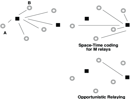
Figure 1: A transmission is overheard by neighboring nodes. Distributed Space-Time coding is needed so that all overhearing nodes could simultaneously transmit. In this work we analyze ”Opportunistic Relaying” where the relay with the strongest transmitter-relay-receiver path is selected, among several candidates, in a distributed fashion using instantaneous channel measurements.

In fig. 1 a transmitter transmits its information towards the receiver while all the neighboring nodes are in listening mode. For a practical cooperative diversity in a three-node setup, the transmitter should know that allowing a relay at location (B) to relay information, would be more efficient than repetition from the transmitter itself. This is not a trivial task and such event depends on the wireless channel conditions between transmitter and receiver as well as between transmitter-relay and relay-receiver. What if the relay is located in position (A)? This problem also manifests in the multiple relay case, when one attempts to simplify the physical layer protocol by choosing the best available relay. In [19] it was suggested that the best relay be selected based on location information with respect to source and destination based on ideas from geographical routing proposed in [17]. Such schemes require knowledge or estimation of distances between all relays and destination and therefore require either a) infrastructure for distance estimation (for example GPS receivers at each terminal) or b) distance estimation using expected SNRs which is itself a non-trivial problem and is more appropriate for static networks and less appropriate for mobile networks, since in the latter case, estimation should be repeated with substantial overhead.

In contrast, we propose a novel scheme that selects the best relay between source and destination based on instantaneous channel measurements. The proposed scheme requires no knowledge of the topology or its estimation. The technique is based on signal strength measurements rather than distance and requires a small fraction of the channel coherence time. All these features make the design of such a scheme highly challenging and the proposed solution becomes non-trivial. Additionally, the algorithm itself provides for the necessary coordination in time and group formation among the cooperating terminals.

The three-node reduction of the multiple relay problem we consider, greatly simplifies the physical layer design. In particular, the requirement of space-time codes is completely eliminated if the source and relay transmit in orthogonal time-slots. We further show that there is essentially no loss in performance in terms of the diversity-multiplexing tradeoff as compared to the transmission scheme in [7] which requires space-time coding across the relays successful in decoding the source message. We also note that our scheme can be used to simplify the non-orthogonal multiple relay protocols studied in [1]. Intuitively, the gains in cooperative diversity do not come from using complex schemes, but rather from the fact that we have enough relays in the system to provide sufficient diversity.

The simplicity of the technique, allows for immediate implementation in existing radio hardware. An implementation of the scheme using custom radio hardware is reported in [3]. Its adoption could provide for improved flexibility (since the technique addresses coordination issues), reliability and efficiency (since the technique inherently builds upon diversity) in future 4G wireless systems.

I-A Key Contributions

One of the key contribution of this paper is to propose and analyze a simplification of user cooperation protocols at the physical layer by using a smart relay selection algorithm at the network layer. Towards this end, we take the following steps:

• A new protocol for selection of the ”best” relay between the source and destination is suggested and analyzed. This protocol has the following features:

  • The protocol is distributed and each relay only makes local channel measurements.

  • Relay selection is based on instantaneous channel conditions in slow fading wireless environments. No prior knowledge of topology or estimation of it is required.

  • The amount of overhead involved in selecting the best relay is minimal. It is shown that there is a flexible tradeoff between the time incurred in the protocol and the resulting error probability.

• The impact of smart relaying on the performance of user cooperation protocols is studied. In particular, it is shown that for orthogonal cooperative diversity protocols there is no loss in performance (in terms of the diversity multiplexing tradeoff) if only the best relay participates in cooperation. Opportunistic relaying provides an alternative solution with a very simple physical layer to conventional cooperative diversity protocols that rely on space-time codes. The scheme could be further used to simplify space-time coding in the case of non-orthogonal transmissions.

Since the communication scheme exploits the wireless channel at its best, via distributed cooperating relays, we naturally called it opportunistic relaying. The term ”opportunistic” has been widely used in various different contexts. In [23], it was used in the context of repetitive transmission of the same information over several paths, in 802.11b networks. In our setup, we do not allow repetition since we are interested in providing diversity without sacrificing the achievable rates, which is a characteristic of repetition schemes. The term ”opportunistic” has also been used in the context of efficient flooding of signals in multi-hop networks [24], to increase communication range and therefore has no relationship with our work. We first encountered the term ”opportunistic” in the work by Viswanath, Tse and Laroia [25], where the base station always selects the best user for transmission in an artificially induced fast fading environment. In our work, a mechanism of multi-user diversity is provided for the relay channel, in single antenna terminals. Our proposed scheme, resembles selection diversity that has been proposed for centralized multi-antenna receivers [8]. In our setup, the single antenna relays are distributed in space and attention has been given in selecting the “best” possible antenna, well before the channel changes again, using minimal communication overhead.

In the following section, we describe in detail opportunistic relaying and contrast its distributed, location information-free nature to existing approaches in the field. Probabilistic analysis and close form expressions regarding the success (or failure) and speed of “best” path selection, for any kind of wireless channel statistics, are provided in section III. In section IV we prove that opportunistic relaying has no performance loss compared to complex space-time coding, under the same assumptions of orthogonal channel transmissions [7] and discuss the ability of the scheme to further simplify space-time coding for non-orthogonal channels. We also discuss in more detail, why space-time codes designed for the MIMO link are not directly applicable to the cooperative relay channel. We conclude in section V.

II Description of Opportunistic Relaying

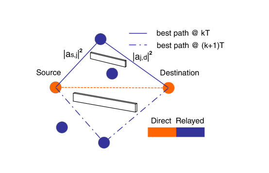
Figure 2: Source transmits to destination and neighboring nodes overhear the communication. The ”best” relay among M candidates is selected to relay information, via a distributed mechanism and based on instantaneous end-to-end channel conditions. For the diversity-multiplexing tradeoff analysis, transmission of source and ”best” relay occur in orthogonal time channels. The scheme could be easily modified to incorporate simultaneous transmissions from source and ”best” relay.

According to opportunistic relaying, a single relay among a set of $M$ relay nodes is selected, depending on which relay provides for the ”best” end-to-end path between source and destination (fig. 1, 2). The wireless channel $a_{si}$ between source and each relay $i$, as well as the channel $a_{id}$ between relay $i$ and destination affect performance. These parameters model the propagation environment between any communicating terminals and change over time, with a rate that macroscopically can be modelled as the Doppler shift, inversely proportional to the channel coherence time. Opportunistic selection of the “best” available relay involves the discovery of the most appropriate relay, in a distributed and “quick” fashion, well before the channel changes again. We will explicitly quantify the speed of relay selection in the following section.

The important point to make here is that under the proposed scheme, the relay nodes monitor the instantaneous channel conditions towards source and destination, and decide in a distributed fashion which one has the strongest path for information relaying, well before the channel changes again. In that way, topology information at the relays (specifically location coordinates of source and destination at each relay) is not needed. The selection process reacts to the physics of wireless propagation, which are in general dependent on several parameters including mobility and distance. By having the network select the relay with the strongest end-to-end path, macroscopic features like “distance” are also taken into account. Moreover, the proposed technique is advantageous over techniques that select the best relay a priori, based on distance toward source or destination, since distance-dependent relay selection neglects well-understood phenomena in wireless propagation such as shadowing or fading: communicating transmitter-receiver pairs with similar distances might have enormous differences in terms of received SNRs. Furthermore, average channel conditions might be less appropriate for mobile terminals than static. Selecting the best available path under such conditions (zero topology information, ”fast” relay selection well bellow the coherence time of the channel and minimum communication overhead) becomes non-obvious and it is one of the main contributions of this work.

More specifically, the relays overhear a single transmission of a Ready-to-Send (RTS) packet and a Clear-to-Send (CTS) packet from the destination. From these packets the relays assess how appropriate each of them is for information relaying. The transmission of RTS from the source allows for the estimation of the instantaneous wireless channel $a_{si}$ between source and relay $i$, at each relay $i$ (fig. 2). Similarly, the transmission of CTS from the destination, allows for the estimation of the instantaneous wireless channel $a_{id}$ between relay $i$ and destination, at each relay $i$, according to the reciprocity theorem[26]. Note that the source does not need to listen to the CTS packet from the destination.

Since communication among all relays should be minimized for reduced overall overhead, a method based on time was selected: as soon as each relay receives the CTS packet, it starts a timer from a parameter $h_{i}$ based on the instantaneous channel measurements $a_{si},a_{id}$. The timer of the relay with the best end-to-end channel conditions will expire first. That relay transmits a short duration flag packet, signaling its presence. All relays, while waiting for their timer to reduce to zero (i.e. to expire) are in listening mode. As soon as they hear another relay to flag its presence or forward information (the best relay), they back off.

For the case where all relays can listen source and destination, but they are ”hidden” from each other (i.e. they can not listen each other), the best relay notifies the destination with a short duration flag packet and the destination notifies all relays with a short broadcast message.

The channel estimates $a_{si},~{}a_{id}$ at each relay, describe the quality of the wireless path between source-relay-destination, for each relay $i$. Since the two hops are both important for end-to-end performance, each relay should quantify its appropriateness as an active relay, using a function that involves the link quality of both hops. Two functions are used in this work: under policy I, the minimum of the two is selected (equation (1)), while under policy II, the harmonic mean of the two is used (equation (2)). Policy I selects the ”bottleneck” of the two paths while Policy II balances the two link strengths and it is a smoother version of the first one.

Under policy I:

$$h_{i}=\min\{|a_{si}|^{2},|a_{id}|^{2}\}$$ (1)

Under policy II:

$$h_{i}=\frac{2}{\frac{1}{|a_{si}|^{2}}+\frac{1}{|a_{id}|^{2}}}=\frac{2~{}|a_{si}|^{2}~{}|a_{id}|^{2}}{|a_{si}|^{2}+|a_{id}|^{2}}$$ (2)

The relay $i$ that maximizes function $h_{i}$ is the one with the ”best” end-to-end path between initial source and final destination. After receiving the CTS packet, each relay $i$ will start its own timer with an initial value $T_{i}$, inversely proportional to the end-to-end channel quality $h_{i}$, according to the following equation:

$$T_{i}=\frac{\lambda}{h_{i}}$$ (3)

Here $\lambda$ is a constant. The units of $\lambda$ depend on the units of $h_{i}$. Since $h_{i}$ is a scalar, $\lambda$ has the units of time. For the discussion in this work, $\lambda$ has simply values of $\mu secs$.

$$h_{b} = \max\{h_{i}\},~{}\Longleftrightarrow$$ (4)

$$T_{b} = \min\{T_{i}\},~{}i~{}\in~{}[1..M].$$ (5)

Therefore, the ”best” relay has its timer reduced to zero first (since it started from a smaller initial value, according to equations (3)-(5). This is the relay $b$ that participates in forwarding information from the source. The rest of the relays, will overhear the ”flag” packet from the best relay (or the destination, in the case of hidden relays) and back off.

After the best relay has been selected, then it can be used to forward information towards the destination. Whether that ”best” relay will transmit simultaneously with the source or not, is completely irrelevant to the relay selection process. However, in the diversity-multiplexing tradeoff analysis in section IV, we strictly allow only one transmission at each time and therefore we can view the overall scheme as a two-step transmission: one from source and one from ”best” relay, during a subsequent (orthogonal) time channel (fig. 2).

II-A A note on Time Synchronization

In principle, the RTS/CTS transmissions between source and destination, existent in many Medium Access Control (MAC) protocols, is only needed so that all intermediate relays can assess their connectivity paths towards source and destination. The reception of the CTS packet triggers at each relay the initiation of the timing process, within an uncertainty interval that depends on different propagation times, identified in detail in section III. Therefore, an explicit time synchronization protocol among the relays is not required. Explicit time synchronization would be needed between source and destination, only if there was no direct link between them. In that case, the destination could not respond with a CTS to a RTS packet from the source, and therefore source and destination would need to schedule their RTS/CTS exchange by other means. In such cases ”crude” time synchronization would be useful. Accurate synchronization schemes, centralized [2] or decentralized [4], do exist and have been studied elsewhere. We will assume that source and destination are in communication range and therefore no synchronization protocols are needed.

II-B A note on Channel State Information (CSI)

CSI at the relays, in the form of link strengths (not signal phases), is used at the network layer for ”best” relay selection. CSI is not required at the physical layer and is not exploited either at the source or the relays. The wireless terminals in this work do not exploit CSI for beamforming and do not adapt their transmission rate to the wireless channel conditions, either because they are operating in the minimum possible rate or because their hardware do not allow multiple rates. We will emphasize again that no CSI at the physical layer is exploited at the source or the relays, during the diversity-multiplexing tradeoff analysis, in section IV.

II-C Comparison with geometric approaches

As can be seen from the above equations, the scheme depends on the instantaneous channel realizations or equivalently, on received instantaneous SNRs, at each relay. An alternative approach would be to have the source know the location of the destination and propagate that information, alongside with its own location information to the relays, using a simple packet that contained that location information. Then, each relay, assuming knowledge of its own location information, could assess its proximity towards source and destination and based on that proximity, contend for the channel with the rest of the relays. That is an idea, proposed by Zorzi and Rao [17] in the context of fading-free wireless networks, when nodes know their location and the location of their destination (for example they are equipped with GPS receivers). The objective there was to study geographical routing and study the average number of hops needed under such schemes. All relays are partitioned into a specific number of geographical regions between source and destination and each relay identifies its region using knowledge of its location and the location of source and destination. Relays at the region closer to the destination contend for the channel first using a standard CSMA splitting scheme. If no relays are found, then relays at the second closest region contend and so on, until all regions are covered, with a typical number of regions close to 4. The latency of the above distance-dependent contention resolution scheme was analyzed in [18].

Zorzi and Rao’s scheme of distance-dependent relay selection was employed in the context of Hybrid-ARQ, proposed by Zhao and Valenti [19]. In that work, the request to an Automatic Repeat Request (ARQ) is served by the relay closest to the destination, among those that have decoded the message. In that case, code combining is assumed that exploits the direct and relayed transmission (that’s why the term Hybrid was used). Relays are assumed to know their distances to the destination (valid for GPS equipped terminals) or estimate their distances by measuring the expected channel conditions using the ARQ requests from the destination or using other means.

We note that our scheme of opportunistic relaying differs from the above scheme in the following aspects:

• The above scheme performs relay selection based on geographical regions while our scheme performs selection based on instantaneous channel conditions. In wireless environment, the latter choice could be more suitable as relay nodes located at similar distance to the destination could have vastly different channel gains due to effects such as fading.

• The above scheme requires measurements to be only performed once if there is no mobility among nodes but requires several rounds of packet exchanges to determine the average SNR. On the other hand opportunistic relaying requires only three packet exchanges in total to determine the instantaneous SNR, but requires that these measurements be repeated in each coherence interval. We show in the subsequent section that the overhead of relay selection is a small fraction of the coherence interval with collision probability less than $0.6\%$.

• We also note that our protocol is a proactive protocol since it selects the best relay before transmission. The protocol can easily be made to be reactive (similar to [19]) by selecting the relay after the first phase. However this modification would require all relays to listen to the source transmission which can be energy inefficient from a network sense.

III Probabilistic Analysis of Opportunistic Relaying

The probability of having two or more relay timers expire ”at the same time” is zero. However, the probability of having two or more relay timers expire within the same time interval $c$ is non zero and can be analytically evaluated, given knowledge of the wireless channel statistics.

The only case where opportunistic relay selection fails is when one relay can not detect that another relay is more appropriate for information forwarding. Note that we have already assumed that all relays can listen initial source and destination, otherwise they do not participate in the scheme. We will assume two extreme cases: a) all relays can listen to each other b) all relays are hidden from each other (but they can listen source and destination). In that case, the flag packet sent by the best relay is received from the destination which responds with a short broadcast packet to all relays. Alternatively, other schemes based on ”busy tone” (secondary frequency) control channels could be used, requiring no broadcast packet from the destination and partly alleviating the ”hidden” relays problem.

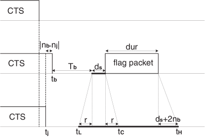
Figure 3: The middle row corresponds to the ”best” relay. Other relays (top or bottom row) could erroneously be selected as ”best” relays, if their timer expired within intervals when they can not hear the best relay transmission. That can happen in the interval $[t_{L},t_{C}]$ for case (a) (No Hidden Relays) or $[t_{L},t_{H}]$ for case (b) (Hidden Relays). $t_{b},t_{j}$ are time points where reception of the CTS packet is completed at best relay $b$ and relay $j$ respectively.

From fig. 3, collision of two or more relays can happen if the best relay timer $T_{b}$ and one or more other relay timers expire within $[t_{L},~{}t_{C}]$ for the case of no hidden relays (case (a)). This interval depends on the radio switch time from receive to transmit mode $d_{s}$ and the propagation times needed for signals to travel in the wireless medium. In custom low-cost transceiver hardware, this switch time is typically on the order of a few $\mu seconds$ while propagation times for a range of 100 meters is on the order of $1/3~{}\mu seconds$. For the case of ”hidden” relays the uncertainty interval becomes $[t_{L},~{}t_{H}]$ since now the duration of the flag packet should be taken into account, as well as the propagation time towards the destination and back towards the relays and the radio switch time at the destination. The duration of the flag packet can be made small, even one bit transmission could suffice. In any case, the higher this uncertainty interval, the higher the probability of two or more relay timers to expire within that interval. That’s why we will assume maximum values of $c$, so that we can assess worst case scenario performance.

(a) No Hidden Relays:

$$c=r_{max}+|n_{b}-n_{j}|_{max}+d_{s}$$ (6)

(b) Hidden Relays:

$$c=r_{max}+|n_{b}-n_{j}|_{max}+2d_{s}+dur+2n_{max}$$ (7)

• $n_{j}$: propagation delay between relay $j$ and destination. $n_{max}$ is the maximum.

• $r$: propagation delay between two relays. $r_{max}$ is the maximum.

• $d_{s}$: receive-to-transmit switch time of each radio.

• $dur$: duration of flag packet, transmitted by ”best” relay.

In any case, the probability of having two or more relays expire within the same interval $c$, out of a collection of $M$ relays, can be described by the following expression:

$$Pr(Collision) \leq Pr(any~{}T_{j}<T_{b}+c~{}|~{}j\neq b)$$ (8)

$$where~{}T_{b} = \min\{T_{j}\},~{}j\in[1,M]~{}and~{}c>0.$$

Notice that we assume failure of relay selection when two or more relays collide. Traditional CSMA protocols would require the relays to sense that collision, back-off and retry. In that way collision probability could be further reduced, at the expense of increased latency overhead for relay selection. We will analyze the collision probability without any contention resolution protocol and further improvements are left for future work.

We will provide an analytic way to calculate a close-form expression of equation (8) for any kind of wireless fading statistics. But before doing so, we can easily show that this probability can be made arbitrary small, close to zero.

If $T_{b}=\min\{T_{j}\},j\in[1,M]$ and $Y_{1}<Y_{2}<\ldots<Y_{M}$ the ordered random variables $\{T_{j}\}$ with $T_{b}\equiv Y_{1}$, and $Y_{2}$ the second minimum timer, then:

$$Pr(any~{}T_{j}<T_{b}+c~{}|~{}j\neq b)\equiv Pr(Y_{2}<Y_{1}+c)$$ (9)

From the last equation, we can see that this probability can be made arbitrarily small by decreasing the parameter $c$. For short range radios (on the order of 100 meters), this is primarily equivalent to selecting radios with small switch times (from receive to transmit mode) on the order of a few microseconds.

Given that $Y_{j}=\lambda/h_{(j)}$, $Y_{1}<Y_{2}<\ldots<Y_{M}$ is equivalent to $1/h_{(1)}<1/h_{(2)}<\ldots<1/h_{(M)}$, equation (9) is equivalent to

$$Pr(Y_{2}<Y_{1}+c)=Pr(\frac{1}{h_{(2)}}<\frac{1}{h_{(1)}}+\frac{c}{\lambda})$$ (10)

and $Y_{1}<Y_{2}<\ldots<Y_{M}\Leftrightarrow h_{(1)}>h_{(2)}\ldots>h_{(M)}$ ($h,\lambda,c$ are positive numbers).

From the last equation (10), it is obvious that increasing $\lambda$ at each relay (in equation (3)), reduces the probability of collision to zero since equation (10) goes to zero with increasing $\lambda$.

In practice, $\lambda$ can not be made arbitrarily large, since it also ”regulates” the expected time, needed for the network to find out the ”best” relay. From equation (3) and Jensen’s inequality we can see that

$$E[T_{j}]=E[\lambda/h_{j}]\geq\lambda/E[h_{j}]$$ (11)

or in other words, the expected time needed for each relay to flag its presence, is lower bounded by $\lambda$ times a constant. Therefore, there is a tradeoff between probability of collision and speed of relay selection. We need to have $\lambda$ as big as possible to reduce collision probability and at the same time, as small as possible, to quickly select the best relay, before the channel changes again (i.e. within the coherence time of the channel). For example, for a mobility of $0-3$ km/h, the maximum Doppler shift is $f_{m}=2.5~{}Hz$ which is equivalent with a minimum coherence time on the order of $200$ milliseconds. Any relay selection should occur well before that time interval with a reasonably small probability of error. From figure 4, we note that selecting $c/\lambda\approx 1/200$ will result in a collision probability less than $0.6\%$ for policy I. Typical switching times result in $c\approx 5\mu s$. This gives $\lambda\approx 1ms$ which is two orders of magnitude less than the coherence interval. More sophisticated radios with $c\approx 1\mu s$ will result in $\lambda\approx 200\mu s$, which is three orders of magnitude smaller than the coherence time .

III-A Calculating $Pr(Y_{2}<Y_{1}+c)$

In order to calculate the collision probability from (9), we first need to calculate the joint probability distribution of the minimum and second minimum of a collection of $M$ i.i.d random variables, corresponding to the timer functions of the $M$ relays. The following theorem provides this joint distribution:

Theorem 1

The joint probability density function of the minimum and second minimum among $M\geq 2$ i.i.d. positive random variables $T_{1},~{}T_{2},\dots,~{}T_{M}$, each with probability density function $f(t)\equiv\frac{dF(t)}{dt}$ and cumulative distribution function $F(t)\equiv Pr(T\leq t)$, is given by the following equation:

$$f_{Y_{1},Y_{2}}(y_{1},y_{2})=\begin{cases}M~{}(M-1)~{}f(y_{1})~{}f(y_{2})~{}[1-F(y_{2})]^{M-2}&for~{}0<y_{1}<y_{2}\\ 0&elsewhere.\end{cases}$$

where $Y_{1}<Y_{2}<Y_{3}\ldots<Y_{M}$ are the $M$ ordered random variables $T_{1},~{}T_{2},\ldots,~{}T_{M}$.

Proof:

Please refer to appendix A. ∎

Using Theorem 1, we can show the following lemma that gives a closed-form expression for the collision probability (equation 9):

Lemma 1

Given $M\geq 2$ i.i.d. positive random variables $T_{1},~{}T_{2},\dots,~{}T_{M}$, each with probability density function $f(x)$ and cumulative distribution function $F(x)$, and $Y_{1}<Y_{2}<Y_{3}\ldots<Y_{M}$ are the $M$ ordered random variables $T_{1},~{}T_{2},\ldots,~{}T_{M}$, then $Pr(Y_{2}<Y_{1}+c)$, where $c>0$, is given by the following equations:

$$Pr(Y_{2}<Y_{1}+c)=1-I_{c}$$ (12)

$$I_{c}=M~{}(M-1)~{}\int_{c}^{+\infty}f(y)~{}[1-F(y)]^{M-2}~{}F(y-c)~{}dy$$ (13)

Proof:

Please refer to appendix A. ∎

Notice that the statistics of each timer $T_{i}$ and the statistics of the wireless channel are related according to equation (3). Therefore, the above formulation is applicable to any kind of wireless channel distribution.

III-B Results

In order to exploit theorem 1 and lemma 1, we first need to calculate the probability distribution of $T_{i}$ for $i~{}\in[1,M]$. From equation (3) it is easy to see that the cdf $F(t)$ and pdf $f(t)$ of $T_{i}$ are related to the respective distributions of $h_{i}$ according to the following equations:

$$F(t)\equiv~{}CDF_{T_{i}}(t)=Pr\{T_{i}~{}\leq~{}t\}=1-CDF_{h_{i}}(\frac{\lambda}{t})$$ (14)

$$f(t)\equiv~{}pdf_{T_{i}}(t)=\frac{d}{dt}F(t)=\frac{\lambda}{t^{2}}~{}pdf_{h_{i}}(\frac{\lambda}{t})$$ (15)

After calculating equations (14), (15), and for a given $c$ calculated from (6) or (7), and a specific $\lambda$, we can calculate probability of collision using equation (12).

Before proceeding to special cases, we need to observe that for a given distribution of the wireless channel, collision performance depends on the ratio $c/\lambda$, as can be seen from equation (10), discussed earlier.

III-B1 Rayleigh Fading

Assuming $|a_{si}|,~{}|a_{id}|$, for any $i\in[1,M]$, are independent (but not identically distributed) Rayleigh random variables, then $|a_{si}|^{2},~{}|a_{id}|^{2}$ are independent, exponential random variables, with parameters $\beta_{1},\beta_{2}$ respectively ($E[|a_{si}|^{2}]=1/\beta_{1},~{}E[|a_{id}|^{2}]=1/\beta_{2}$).

Using the fact that the minimum of two independent exponential r.v.’s with parameters $\beta_{1},\beta_{2}$, is again an exponential r.v with parameter $\beta_{1}+\beta_{2}$, we can calculate the distributions for $h_{i}$ under policy I (equation 1). For policy II (equation 2), the distributions of the harmonic mean, have been calculated analytically in [5]. Equations (14) and (15) become:

under policy I:

$$F(t) = e^{-~{}(\beta_{1}+\beta_{2})~{}\lambda/t}$$ (16)

$$f(t) = \frac{~{}\lambda~{}(\beta_{1}+\beta_{2})}{t^{2}}~{}e^{-(\beta_{1}+\beta_{2})~{}\lambda/t}$$ (17)

under policy II:

$$F(t) = \frac{\lambda~{}\sqrt{\beta_{1}~{}\beta_{2}}}{t}~{}e^{-\lambda~{}(\beta_{1}+\beta_{2})/(2t)}~{}K_{1}({\frac{\lambda~{}\sqrt{\beta_{1}\beta_{2}}}{t}})$$ (18)

$$f(t) = ~{}\frac{\lambda^{2}}{2~{}t^{3}}~{}\beta_{1}~{}\beta_{2}~{}e^{-\lambda~{}(\beta_{1}+\beta_{2})/(2t)}~{}[\frac{\beta_{1}+\beta_{2}}{\sqrt{\beta_{1}~{}\beta_{2}}}K_{1}({\frac{\lambda~{}\sqrt{\beta_{1}~{}\beta_{2}}}{t}})+2~{}K_{0}({\frac{\lambda~{}\sqrt{\beta_{1}~{}\beta_{2}}}{t}})]$$ (19)

where $K_{i}(x)$ is the modified Bessel function of the second kind and order $i$.

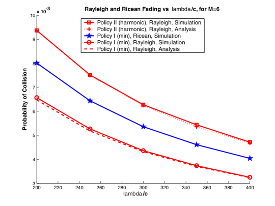
Figure 4: Performance in Rayleigh and Ricean fading, for policy I (min) and Policy II (harmonic mean), various values of ratio $\lambda/c$ and $M=6$ relays, clustered at the same region. Notice that collision probability drops well below $1\%$.

Equation (12) is calculated for the two policies, for the symmetric case ($\beta_{1}=\beta_{2}=E[|a_{si}|^{2}]=E[|a_{id}|^{2}]=1$) of $M=6$ relays. Monte-Carlo simulations are also performed under the same assumptions. Results are plotted in fig. 4, for various ratios $\lambda/c$. We can see that Monte-carlo simulations match the results provided by numerical calculation of equation (12) with the help of equations (16)-(19).

Collision probability drops with increasing ratio of $\lambda/c$ as expected. Policy I (”the minimum”), performs significantly better than Policy II (”the harmonic mean”) and that can be attributed to the fact that the harmonic mean smooths the two path SNRs (between source-relay and relay-destination) compared to the minimum function. Therefore, the effect of randomization due to fading among the relay timers, becomes less prominent under Policy II. The probability can be kept well below $1\%$, for ratio $\lambda/c$ above $200$.

III-B2 Ricean Fading

It was interesting to examine the performance of opportunistic relay selection, in the case of Ricean fading, when there is a dominating communication path between any two communicating points, in addition to many reflecting paths and compare it to Rayleigh fading, where there is a large number of equal power, independent paths.

Keeping the average value of any channel coefficient the same ($E[|a|^{2}]=1$) and assuming a single dominating path and a sum of reflecting paths (both terms with equal total power), we plotted the performance of the scheme when policy I was used, using Monte-Carlo simulations (fig. 4). We can see that in the Ricean case, the collision probability slightly increases, since now, the realizations of the wireless paths along different relays are clustered around the dominating path and vary less, compared to Rayleigh fading. Policy II performs slightly worse, for the same reasons it performed slightly worse in the Rayleigh fading case and the results have been omitted.

In either cases of wireless fading (Rayleigh or Ricean), the scheme performs reasonably well.

III-B3 Different topologies

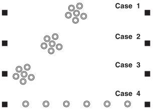
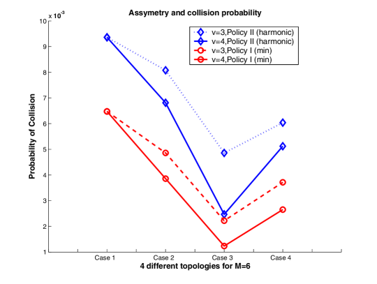
Figure 5: Unequal expected values (moments) among the two path SNRs or among the relays, reduce collision probability. M=6 and $c/\lambda=1/200$ for the four different topologies considered.

For the case of all relays not equidistant to source or destination, we expect the collision probability to drop, compared to the equidistant case, since the asymmetry between the two links (from source to relay and from relay to destination) or the asymmetry between the expected SNRs among the relays, will increase the variance of the timer function, compared to the equidistant case. To demonstrate that, we studied three cases, where $M=6$ relays are clustered half-way ($d/2$), closer to transmitter ($d/3$) or even closer to transmitter ($d/10$) (case 1,2,3 respectively in fig. 5 and $d$ is the distance between source and destination) and one case where the relays form an equidistant line network between source and destination (case 4 in fig. 5).

Assuming Rayleigh fading, $c/\lambda=1/200$ and expected path strength as a non-linear, decreasing function of distance ($E[|a_{ij}|^{2}]=1/\beta_{ij}\propto(1/d_{ij})^{v}$), we calculated the collision probability for $M=6$ relays, using expressions (16)-(19) into (12) for cases 1, 2, 3 while for case 4 we used Monte-Carlo simulation: in case 1, $\beta_{1}=\beta_{2}=1$, in case 2, $\beta_{1}=(2/3)^{v},\beta_{2}=(4/3)^{v}$ and in case 3, $\beta_{1}=(1/5)^{v},\beta_{2}=(9/5)^{v}$. For case 4, $\beta_{1}=(2/7)^{v},\beta_{2}=(12/7)^{v}$ for the closest terminal to source, $\beta_{1}=(4/7)^{v},\beta_{2}=(10/7)^{v}$ for the second closest terminal to source, $\beta_{1}=(6/7)^{v},\beta_{2}=(8/7)^{v}$ for the third closest to source terminal. Due to symmetry, the expected power and corresponding $\beta$ factors of the paths, for the third closer to destination, second closer to destination and closest terminal to destination, are the same with the ones described before (third closer terminal to source, second closer terminal to source and closest to source terminal respectively), with $\beta_{1}$ and $\beta_{2}$ interchanged.

From fig. 5, we can see that the collision probability of asymmetric cases 2, 3 and 4 is strictly smaller compared to the symmetric case 1. Policy I performs better than Policy II and collision probability decreases for increasing factor $v$ ($v=3,4$ were tested). This observation agrees with intuition that suggests that different moments for the path strengths among the relays, increase the randomness of the expiration times among the relays and therefore decrease the probability of having two or more timers expire within the same time interval.

We note that the source can also participate in the process of deciding the best relay. In this special case, where the source can receive the CTS message, it could have its own timer start from a value depending upon the instantaneous $|a_{sd}|^{2}$. This will be important if the source is not aware whether there are any relays in the vicinity that could potentially cooperate.

The proposed method as described above, involving instantaneous SNRs as a starting point for each relay’s timer and using time (corresponding to an assessment of how good is a particular path within the coherence time of the channel) to select space (the best available path towards destination) in a distributed fashion, is novel and has not been proposed before, to the best extent of our knowledge.

IV Simplifying Cooperative Diversity through Opportunistic Relaying

We now consider the impact of opportunistic relaying on the cooperative diversity scenario. The main result of this section is that opportunistic relaying can be used to simplify a number of cooperative diversity protocols involving multiple relays. In particular we focus on the cooperative diversity protocol in [7] which requires the relays to use a space-time code while simultaneously transmitting towards the destination. We show that this protocol can be simplified considerably by simply selecting the best relay in the second stage. Perhaps surprisingly, this simplified protocol achieves the same diversity multiplexing tradeoff achieved in [7]. Furthermore, it does not matter whether the relay implements an amplify and forward or a decode and forward protocol in terms of the diversity-multiplexing tradeoff. We also note that opportunistic relaying can be used to simplify the non-orthogonal relaying protocols proposed in [1]. However the detailed performance analysis is left for future work.

IV-A Channel Model

We consider an i.i.d slow Rayleigh fading channel model following [6]. A half duplex constraint is imposed across each relay node, i.e. it cannot transmit and listen simultaneously. We assume that the nodes (transmitter and relays) do not exploit the knowledge of the channel at the physical layer. Note that in the process of discovering the best relay described in the previous section the nodes do learn about their channel gains to the destination. However, we assume that this knowledge of channel gain is limited to the network layer protocol. The knowledge of channel gain is not exploited at the physical layer in order to adjust the code rate based on instantaneous channel measurements. In practice, the hardware at the physical layer could be quite constrained to allow for this flexibility to change the rate on the fly. It could also be that the transmitter is operating at the minimum transmission rate allowed by the radio hardware. Throughout this section, we assume that the channel knowledge is not exploited at the physical layer at either the transmitter or the relays.

If the discrete time received signal at the destination and the relay node are denoted by $Y[n]$ and $Y_{1}[n]$ respectively:

$$Y[n] = {a_{sd}}X[n]+Z[n],~{}~{}~{}n=1,2\ldots\frac{T}{2}~{}~{}~{}\text{(source~{}transmits~{}destination~{}receives)}$$ (20)

$$Y[n] = {a_{rd}}X_{1}[n]+Z[n],~{}~{}~{}n=\frac{T}{2},\frac{T}{2}+1\ldots,T~{}~{}\text{(best~{}relay~{}transmits~{}destination~{}receives)}$$ (21)

$$Y_{1}[n] = {a_{sr}}X[n]+Z_{1}[n]~{}~{}~{}n=1,2\ldots\frac{T}{2}~{}~{}~{}\text{(source~{}transmits~{}best~{}relay~{}receives)}$$ (22)

Here ${a_{sd}},{a_{rd}},{a_{sr}}$ are the respective channel gains from the source to destination, best relay to destination and source to the best relay respectively. The channel gains between any two pair of nodes are i.i.d ${\mathcal{N}}(0,1)$. The noise $Z[n]$ and $Z_{1}[n]$ at the destination and relay are both assumed to be i.i.d circularly symmetric complex Gaussian ${\mathcal{N}}(0,\sigma^{2})$. $X[n]$ and $X_{1}[n]$ are the transmitted symbols at the transmitter and relay respectively. $T$ denotes the duration of time-slots reserved for each message and we assume that the source and the relay each transmit orthogonally on half of the time-slots. We impose a power constraint at both the source and the relay: $E[|X[n]|^{2}]\leq P$ and $E[|X_{1}[n]|^{2}]\leq P$. For simplicity, we assume that both the source and the relay to have the same power constraint. We will define $\rho\stackrel{{\scriptstyle\Delta}}{{=}}P/\sigma^{2}$ to be the effective signal to noise ratio (SNR). This setting can be easily generalized when the power at the source and relays is different.

The following notation is necessary in the subsequent sections of the paper. This notation is along the lines of [1] and simplifies the exposition.

Definition 1

A function $f(\rho)$ is said to be exponentially equal to $b$, denoted by $f(\rho)\doteq\rho^{b}$, if

$$\lim_{\rho\rightarrow\infty}\frac{\log f(\rho)}{\log\rho}=b.$$ (23)

We can define the relation $\stackrel{{\scriptstyle.}}{{\leq}}$ in a similar fashion.

Definition 2

The exponential order of a random variable $X$ with a non-negative support is given by,

$$V=-\lim_{\rho\rightarrow\infty}\frac{\log X}{\log\rho}.$$ (24)

The exponential order greatly simplifies the analysis of outage events while deriving the diversity multiplexing tradeoff. Some properties of the exponential order are derived in Appendix B, lemma 2.

Definition 3

(Diversity-Multiplexing Tradeoff) We use the definition given in [11]. Consider a family of codes $C_{\rho}$ operating at SNR $\rho$ and having rates $R(\rho)$ bits per channel use. If $P_{e}(R)$ is the outage probability (see [9]) of the channel for rate $R$, then the multiplexing gain $r$ and diversity order $d$ are defined as

$$r\stackrel{{\scriptstyle\Delta}}{{=}}\lim_{\rho\rightarrow\infty}\frac{R(\rho)}{\log\rho}$$

$$d\stackrel{{\scriptstyle\Delta}}{{=}}-\lim_{\rho\rightarrow\infty}\frac{\log P_{e}(R)}{\log\rho}\\ \\$$ (25)

What remains to be specified is a policy for selecting the best relay. We essentially use the policy 1 (equation (1)) in the previous section.

Policy 1

Among all the available relays, denote the relay with the largest value of $\min\{{|a_{sr}|}^{2},{|a_{rd}|}2\}$ as the best relay.

To justify this choice, we note from fig. 3 that the performance of policy I is slightly better than policy II. Furthermore, we will see in this section that this choice is optimum in that it enables opportunistic relaying to achieve the same diversity multiplexing tradeoff of more complex orthogonal relaying schemes in [7]. We next discuss the performance of the amplify and forward and decode and forward protocols.

IV-B Digital Relaying - Decode and Forward Protocol

We will first study the case where the intermediate relays have the ability to decode the received signal, re-encode and transmit it to the destination. We will study the protocol proposed in [7] and show that it can be considerably simplified through opportunistic relaying.

The decode and forward algorithm considered in [7] is briefly summarized as follows. In the first half time-slots the source transmits and all the relays and receiver nodes listen to this transmission. Thereafter all the relays that are successful in decoding the message, re-encode the message using a distributed space-time protocol and collaboratively transmit it to the destination. The destination decodes the message at the end of the second time-slot. Note that the source does not transmit in the second half time-slots. The main result for the decode and forward protocol is given in the following theorem :

Theorem 2 ([7])

The achievable diversity multiplexing tradeoff for the decode and forward strategy with $M$ intermediate relay nodes is given by $d(r)=(M+1)(1-2r)$ for $r\in(0,0.5)$.

The following Theorem shows that opportunistic relaying achieves the same diversity-multiplexing tradeoff if the best relay selected according to policy 1.

Theorem 3

Under opportunistic relaying, the decode and forward protocol with $M$ intermediate relays achieves the same diversity multiplexing tradeoff stated in Theorem 2.

Proof:

We follow along the lines of [7]. Let ${\cal E}$ denote the event that the relay is successful in decoding the message at the end of the first half of transmission and $\bar{{\cal E}}$ denote the event that the relay is not successful in decoding the message. Event $\bar{{\cal E}}$ happens when the mutual information between source and best relay drops below the code rate. Suppose that we select a code with rate $R=r\log\rho$ and let $I(X;Y)$ denote the mutual information between the source and the destination. The probability of outage is given by

$$P_{e} = \Pr(I(X;Y)\leq r\log\rho|{\cal E})\Pr({\cal E})+\Pr(I(X;Y)\leq r\log\rho|\bar{{\cal E}})\Pr(\bar{{\cal E}})$$

$$= \Pr\left(\frac{1}{2}\log(1+\rho({|a_{sd}|}^{2}+{|a_{rd}|}^{2}))\leq r\log\rho\right)\Pr({\cal E})+$$

$$\Pr\left(\frac{1}{2}\log(1+\rho{|a_{sd}|}^{2})\leq r\log\rho\right)\Pr(\bar{{\cal E}})$$

$$\leq \Pr\left(\frac{1}{2}\log(1+\rho({|a_{sd}|}^{2}+{|a_{rd}|}^{2}))\leq r\log\rho\right)+$$

$$\Pr\left(\frac{1}{2}\log(1+\rho{|a_{sd}|}^{2})\leq r\log\rho\right)\Pr\left(\frac{1}{2}\log(1+\rho{|a_{sr}|}^{2})\leq r\log\rho\right)$$

$$\leq \Pr\left({|a_{sd}|}^{2}+{|a_{rd}|}^{2}\leq\rho^{2r-1}\right)+\Pr\left({|a_{sd}|}^{2}\leq\rho^{2r-1}\right)\Pr\left({|a_{sr}|}^{2}\leq\rho^{2r-1}\right)$$

$$\leq \Pr\left({|a_{sd}|}^{2}\leq\rho^{2r-1}\right)\Pr\left({|a_{rd}|}^{2}\leq\rho^{2r-1}\right)+\Pr\left({|a_{sd}|}^{2}\leq\rho^{2r-1}\right)\Pr\left({|a_{sr}|}^{2}\leq\rho^{2r-1}\right)$$

$${\stackrel{{\scriptstyle.}}{{\leq}}} \rho^{2r-1}\rho^{M(2r-1)}+\rho^{2r-1}\rho^{M(2r-1)}\doteq\rho^{(M+1)(2r-1)}$$

In the last step we have used claim 2 of Lemma 3 in the appendix with $m=M$.

∎

We next study the performance under analog relaying and then mention several remarks.

IV-C Analog relaying - Basic Amplify and Forward

We will now consider the case where the intermediate relays are not able to decode the message, but can only scale their received transmission (due to the power constraint) and send it to the destination.

The basic amplify and forward protocol was studied in [6] for the case of a single relay. The source broadcasts the message for first half time-slots. In the second half time-slots the relay simply amplifies the signals it received in the first half time-slots. Thus the destination receives two copies of each symbol. One directly from the source and the other via the relay. At the end of the transmission, the destination then combines the two copies of each symbol through a matched filter. Assuming i.i.d Gaussian codebook, the mutual information between the source and the destination can be shown to be [6],

$$I(X;Y) = \frac{1}{2}\log\left(1+\rho{|a_{sd}|}^{2}+f(\rho{|a_{sr}|}^{2},\rho{|a_{rd}|}^{2})\right)$$ (26)

$$f(a,b) = \frac{ab}{a+b+1}$$ (27)

The amplify and forward strategy does not generalize in the same manner as the decode and forward strategy for the case of multiple relays. We do not gain by having all the relay nodes amplify in the second half of the time-slot. This is because at the destination we do not receive a coherent summation of the channel gains from the different receivers. If $\gamma_{j}$ is the scaling constant of receiver $j$, then the received signal will be given by $y[n]=\left(\sum_{j=1}^{M}\gamma_{j}a_{rd}^{j}\right)x[n]+z[n].$ Since this is simply a linear summation of Gaussian random variables, we do not see the diversity gain from the relays. A possible alternative is to have the $M$ relays amplify in a round-robin fashion. Each relay transmits only one out of every $M$ symbols in a round robin fashion. This strategy has been proposed in [7], but the achievable diversity-multiplexing tradeoff is not analyzed.

Opportunistic relaying on the other hand provides another possible solution to analog relaying. Only the best relay (according to policy 1) is selected for transmission. The following theorem shows that opportunistic relaying achieves the same diversity multiplexing tradeoff as that achieved by the (more complicated) decode and forward scheme.

Theorem 4

Opportunistic amplify and forward achieves the same diversity multiplexing tradeoff stated in Theorem 2.

Proof:

We begin with the expression for mutual information between the source and destination (26). An outage occurs if this mutual information is less than the code rate $r\log\rho$. Thus we have that

$$P_{e} = \Pr\left(I(X;Y)\leq r\log\rho\right)$$

$$= \Pr\left(\log(1+\rho{|a_{sd}|}^{2}+f(\rho{|a_{sr}|}^{2},\rho{|a_{rd}|}^{2})\leq 2r\log\rho\right)$$

$$\leq \Pr\left({|a_{sd}|}^{2}\leq\rho^{2r-1},f(\rho{|a_{sr}|}^{2},\rho{|a_{rd}|}^{2})\leq\rho^{2r}\right)$$

$$\stackrel{{\scriptstyle(a)}}{{\leq}} \Pr\left({|a_{sd}|}^{2}\leq\rho^{2r-1},\min{({|a_{sr}|}^{2},{|a_{rd}|}^{2})}\leq\rho^{2r-1}+\rho^{r-1}\sqrt{1+\rho^{2r}}\right)$$

$$\stackrel{{\scriptstyle(b)}}{{\doteq}} \rho^{2r-1}\rho^{M(2r-1)}=\rho^{(M+1)(2r-1)}$$

Here (a) follows from Lemma 4 and (b) follows from Lemma 3, claim 1 in appendix B and the fact that $\rho^{r-1}\sqrt{1+\rho^{2r}}\rightarrow\rho^{2r-1}$ as $\rho\rightarrow\infty$. ∎

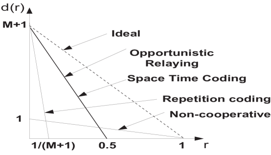
Figure 6: The diversity-multiplexing of opportunistic relaying is exactly the same with that of more complex space-time coded protocols.

IV-D Discussion

IV-D1 Space-time Coding vs. Relaying Solutions

The (conventional) cooperative diversity setup (e.g. [7]) assumes that the cooperating relays use a distributed space-time code to achieve the diversity multiplexing tradeoff in Theorem 2. Development of practical space-time codes is an active area of research. Recently there has been considerable progress towards developing practical codes that achieve the diversity multiplexing tradeoff over MIMO channels. In particular it is known that random lattice based codes (LAST) can achieve the entire diversity multiplexing tradeoff over MIMO channels [16]. Moreover it is noted in [20] that under certain conditions the analytical criterion such as rank and determinant criterion for MIMO links also carry over to cooperative diversity systems . However some practical challenges will have to be addressed to use these codes in the distributed antenna setting: (a) The codes for MIMO channels assume a fixed number of transmit and receive antennas. In cooperative diversity, the number of antennas depends on which relays are successful in decoding and hence is a variable quantity. (b) The destination must be informed either explicitly or implicitly which relays are transmitting.

Opportunistic relaying provides an alternative solution to space time codes for cooperative diversity by using a clever relaying protocol. The result of Theorem 4 suggests that there is no loss in diversity multiplexing tradeoff if a simple analog relaying based scheme is used in conjunction with opportunistic relaying. Even if the intermediate relays are digital, a very simple decode and forward scheme that does eliminates the need for space-time codes can be implemented. The relay listens and decodes the message in the first half of the time-slots and repeats the source transmission in the second half of the time-slots when the source is not transmitting. The receiver simply does a maximal ratio combining of the source and relay transmissions and attempts to decode the message. Theorem 3 asserts that once again the combination of this simple physical layer scheme and the smart choice of the relay is essentially optimum.

The diversity-multiplexing tradeoff is plotted in fig. 6. Even though a single terminal with the “best” end-to-end channel conditions relays the information, the diversity order in the high SNR regime is on the order of the number $M+1$ of all participating terminals. Moreover, the tradeoff is exactly the same with that when space-time coding across $M$ relays is used.

IV-D2 Non-orthogonal Cooperative Diversity Schemes

The focus in this paper was on the multiple relay cooperative diversity protocols proposed in [7], since they require that the transmitter and relay operate in orthogonal time-slots in addition to the half duplex constraints. The orthogonality assumption was amenable to practical implementation [3], since the decoder is extremely simple. More recently, a new class of protocols that relax the assumption that the transmitter and relay operate in orthogonal time-slots, (but still assume the half duplex constraint) have been proposed in [1]. These protocols have a superior performance compared to [7], albeit at the cost of higher complexity both at the decoder and network layer. Opportunistic relaying could be naturally used to simplify those protocols and details of such simplifications and its performance are underway.

IV-D3 Impact of Topology

The analysis in for diversity-multiplexing tradeoff was presented assuming that average channel gains between each pair of nodes is unity. In other words the impact of topology was not considered. We observe that the effect of topology can be included in the analysis using techniques used in [6]. In the high SNR regime, we expect fixed multiplicative factors of path loss to contribute little in affecting the diversity-multiplexing tradeoff. However topology is certainly important for finite SNR case as observed in [22].

V Conclusion

We proposed Opportunistic Relaying as a practical scheme for cooperative diversity. The scheme relies on distributed path selection considering instantaneous end-to-end wireless channel conditions, facilitates coordination among the cooperating terminals with minimum overhead and could simplify the physical layer in communicating transceivers by eliminating the requirement of space time codes.

We presented a method to calculate the performance of the relay selection algorithm, for any kind of wireless fading model and showed that successful relay selection could be engineered with reasonable performance. Specific examples for Rayleigh and Ricean fading were given.

We treated Opportunistic Relaying as a distributed virtual antenna array system and analyzed its diversity-multiplexing tradeoff, revealing NO performance loss when compared with complex space-time coding protocols in the field.

The approach presented in this work explicitly addresses coordination among the cooperating terminals and has similarities with a Medium Access Protocol (MAC) since it directs when a specific node to relay. The algorithm has also similarities with a Routing Protocol since it coordinates which node to relay (or not) received information among a collection of candidates. Devising wireless systems that dynamically adapt to the wireless channel conditions without external means (for example GPS receivers), in a distributed manner, similarly to the ideas presented in this work, is an important and fruitful area for future research.

The simplicity of the technique, allows for immediate implementation in existing radio hardware and its adoption could provide for improved flexibility, reliability and efficiency in future 4G wireless systems.

Appendix A Probabilistic Analysis of Successful Path Selection

Theorem 1 The joint probability density function of the minimum and second minimum among $M$ i.i.d. positive random variables $X_{1},~{}X_{2},\dots,~{}X_{M}$, each with probability density function $f(x)$ and cumulative distribution function $F(x)$, is given by the following equation:

$$f_{Y_{1},Y_{2}}(y_{1},y_{2})=\begin{cases}M~{}(M-1)~{}f(y_{1})~{}f(y_{2})~{}[1-F(y_{2})]^{M-2}&for~{}0<y_{1}<y_{2}\\ 0&elsewhere.\end{cases}$$

where $Y_{1}<Y_{2}<Y_{3}\ldots<Y_{M}$ are the $M$ ordered random variables $X_{1},~{}X_{2},\ldots,~{}X_{M}$.

Proof:

$f_{Y_{1},Y_{2}}(y_{1},y_{2})~{}dy_{1}~{}dy_{2}=Pr(Y_{1}~{}\in~{}dy_{1},~{}Y_{2}~{}\in dy_{2})=\\ Pr(one~{}X_{i}~{}in~{}dy_{1},~{}one~{}X_{j}~{}in~{}dy_{2}~{}(with~{}y_{2}>y_{1}~{}and~{}i\neq j),~{}and~{}all~{}the~{}rest~{}X_{i}^{\prime}s~{}greater~{}than~{}y_{2})=\\ =~{}2~{}\binom{M}{2}~{}Pr(~{}X_{1}\in dy_{1},~{}X_{2}\in dy_{2}~{}(y_{2}>y_{1}),~{}X_{i}>y_{2},~{}i\in~{}[3,M])~{}=\\ =~{}2~{}\binom{M}{2}f(y_{1})~{}dy_{1}~{}f(y_{2})~{}dy_{2}~{}[1-F(y_{2})]^{M-2}=\\ =~{}M~{}(M-1)~{}f(y_{1})~{}f(y_{2})~{}[1-F(y_{2})]^{M-2}~{}dy_{1}~{}dy_{2},~{}for~{}0<y_{1}<y_{2}.$

The third equality is true since there are $\binom{M}{2}$ pairs in a set of M i.i.d. random variables. The factor 2 comes from the fact that ordering in each pair matters, hence we have a total number of $2~{}\binom{M}{2}$ cases, with the same probability, assuming identically distributed random variables. That concludes the proof. ∎

Using Theorem 1, we can prove the following lemma:

Figure 7: Regions of integration of $f_{Y_{1},Y_{2}}(y_{1},y_{2})$, for $Y_{1}<Y_{2}$ needed in Lemma I for calculation of $Pr(Y_{2}<Y_{1}+c),~{}c>0$.

Lemma 1 Given $M$ i.i.d. positive random variables $X_{1},~{}X_{2},\dots,~{}X_{M}$, each with probability density function $f(x)$ and cumulative distribution function $F(x)$, and $Y_{1}<Y_{2}<Y_{3}\ldots<Y_{M}$ the $M$ ordered random variables $X_{1},~{}X_{2},\ldots,~{}X_{M}$, then $Pr(Y_{2}<Y_{1}+c)$, where $c>0$, is given by the following equations:

$$Pr(Y_{2}<Y_{1}+c)=1-I_{c}$$ (28)

$$I_{c}=M~{}(M-1)~{}\int_{c}^{+\infty}f(y)~{}[1-F(y)]^{M-2}~{}F(y-c)~{}dy$$ (29)

Proof:

The joint pdf $f_{Y_{1},Y_{2}}(y_{1},y_{2})$ integrates to $1$ in the region $D\cup D_{c}$, as it can be seen in fig. 7. Therefore:

$$Pr(~{}Y_{2}<Y_{1}+c) = \int\int_{D}~{}f_{Y_{1},Y_{2}}(y_{1},y_{2})~{}dy1~{}dy2$$

$$= 1-\int\int_{D_{c}}~{}f_{Y_{1},Y_{2}}(y_{1},y_{2})~{}dy1~{}dy2$$

$$= 1-I_{c}$$

Again from fig. 7, $I_{c}$ can easily be calculated:

$$I_{c}=\scriptstyle~{}M(M-1)~{}\displaystyle\int_{y_{2}=c}^{+\infty}f(y_{2})~{}[1-F(y_{2})]^{M-2}~{}\int_{0}^{y_{2}-c}f(y_{1})~{}dy_{1}~{}dy_{2}$$

$$=\scriptstyle~{}M(M-1)\displaystyle~{}\int_{y_{2}=c}^{+\infty}f(y_{2})~{}[1-F(y_{2})]^{M-2}~{}F(y_{2}-c)~{}dy_{2}$$ (30)

The last equation concludes the proof. ∎

Appendix B Diversity-Multiplexing Tradeoff Analysis

We repeat Definition 1 and Definition 2 in this section for completeness. The relevant lemmas follow.

Definition 1: A function $f(\rho)$ is said to be exponentially equal to $b$, denoted by $f(\rho)\doteq\rho^{b}$, if

$$\lim_{\rho\rightarrow\infty}\frac{\log f(\rho)}{\log\rho}=b.$$ (31)

We can define the relation $\stackrel{{\scriptstyle.}}{{\leq}}$ in a similar fashion. Definition 2: The exponential order of a random variable $X$ with a non-negative support is given by,

$$V=-\lim_{\rho\rightarrow\infty}\frac{\log X}{\log\rho}.$$ (32)

Lemma 2

Suppose $X_{1},X_{2},\ldots,X_{m}$ are $m$ i.i.d exponential random variables with parameter $\lambda$ (mean $1/\lambda)$, and $X=\max\{X_{1},X_{2},\ldots X_{m}\}$. If $V$ is the exponential order of $X$ then the density function of $V$ is given by

$$f_{V}(v)\doteq\begin{cases}\rho^{-mv}&v\geq 0\\ 0&v<0\end{cases}$$ (33)

and

$$\Pr(X\leq\rho^{-v})\doteq\rho^{-mv}$$ (34)

Proof:

Define,

$$V_{\rho}=-\frac{\log X}{\log\rho}.$$

Thus $V_{\rho}$ is obtained from definition 2, without the limit of $\rho\rightarrow\infty$.

$$\Pr(V_{\rho}\geq v) = \Pr(X\leq\rho^{-v})$$

$$= \Pr(X_{1}\leq\rho^{-v},X_{2}\leq\rho^{-v},\ldots X_{m}\leq\rho^{-v})$$

$$= \prod_{i=1}^{m}\Pr(X_{i}\leq\rho^{-v})$$

$$= \left(1-\exp(-\lambda\rho^{-v})\right)^{m}$$

$$= \left(\lambda\rho^{-v}+\sum_{j=2}^{\infty}\frac{(-\lambda)^{j}}{j!}~{}\rho^{-jv}\right)^{m}$$

Note that $\Pr(V_{\rho}\geq v)\approx\rho^{-mv}$. Differentiating with respect to $v$ and then taking the limit $\rho\rightarrow\infty$, we recover (33). ∎

From the above it can be seen that for the simple case of a single exponential random variable ($m=1$), $\Pr(X\leq\rho^{-v})=\Pr(V_{\rho}\geq v)\doteq\rho^{-v}$.

Lemma 3

For relays, $j=1,2,\ldots,m$, let $a_{sj}$ and $a_{jd}$ denote the channel gains from source to relay $j$ and relay $j$ to destination. Suppose that ${a_{sr}}$ and ${a_{rd}}$ denote the channel gain of the source to the best relay and the best relay to the destination, where the relay is chosen according to rule 1. i.e.

$$\min({|a_{sr}|}^{2},{|a_{rd}|}^{2})=\max\{\min(|a_{s1}|^{2},|a_{1d}|^{2}),\ldots,\min(|a_{sm}|^{2},|a_{md}|^{2})\}$$

Then,

1. $\min({|a_{sr}|}^{2},{|a_{rd}|}^{2})$ has an exponential order given by (33).

2. $$\Pr({|a_{sr}|}^{2}\leq\rho^{-v})=\Pr({|a_{rd}|}^{2}\leq\rho^{-v})\stackrel{{\scriptstyle.}}{{\leq}}\begin{cases}\rho^{-mv}&{v\geq 0}\\ 1&\text{otherwise}\end{cases}$$

Proof:

Let us denote $X^{(j)}\stackrel{{\scriptstyle\Delta}}{{=}}\min(|a_{sj}|^{2},|a_{jd}|^{2})$. Since each of the $X^{(j)}$ are exponential random variables with parameter 2, claim 1 follows from Lemma 2. Also since ${|a_{sd}|}^{2}$ and ${|a_{rd}|}^{2}$ cannot be less than $\min({|a_{sd}|}^{2},{|a_{rd}|}^{2})$ claim 2 follows immediately from claim 1. ∎

Lemma 4

With $f(\cdot,\cdot)$ defined by relation (27), we have that
$~{}~{}~{}~{}~{}~{}~{}~{}~{}~{}~{}~{}~{}~{}~{}~{}~{}~{}\Pr\left(f(\rho a,\rho b)\leq\rho^{2r}\right)\leq\Pr\left(\min(a,b)\leq\rho^{2r-1}+\rho^{r-1}\sqrt{1+\rho^{2r}}\right)$.

Proof:

Without loss in generality, assume that $a\geq b$.

$$f(\rho a,\rho b) = \rho\frac{ab}{a+b+\frac{1}{\rho}}$$

$$= \rho b\left(\frac{a}{a+b+\frac{1}{\rho}}\right)$$

$$\stackrel{{\scriptstyle(a)}}{{\geq}} \rho b\left(\frac{b}{2b+\frac{1}{\rho}}\right)$$

Here (a) follows since $\frac{a}{a+K}$ is an increasing function in $a$, for $K>0$ and $a\geq b$.

Now we have that

$$\Pr\left(f(\rho a,\rho b\right)\leq\rho^{2r}) \leq \Pr\left(\frac{b^{2}}{2b+\frac{1}{\rho}}\leq\rho^{2r-1}\right)$$

$$= \Pr\left(b^{2}\leq 2\rho^{2r-1}b+\rho^{2r-2}\right)$$

$$= \Pr\left((b-\rho^{2r-1})2\leq\rho^{4r-2}+\rho^{2r-2}\right)$$

$$\stackrel{{\scriptstyle(a)}}{{=}} \Pr\left(b\leq\rho^{2r-1}+\rho^{r-1}\sqrt{1+\rho^{2r}}\right)$$

Where (a) follows since $b\geq 0$ so that $\Pr(b<0)=0$.

∎

References

- [1] K. Azarian, H. E. Gamal, and P. Schniter, “On the Achievable Diversity-vs-multiplexing Tradeoff in Cooperative Channels,” IEEE Trans. Information Theory, submitted, 2004.
- [2] A. Bletsas, “Evaluation of Kalman Filtering for Network Time Keeping”, IEEE Transactions on Ultrasonics, Ferromagnetics and Frequency Control, to appear. Available at http://web.media.mit.edu/ aggelos/papers/tuffc_nov04.pdf
- [3] A. Bletsas, Intelligent Antenna Sharing and User Cooperation in Wireless Networks, Ph.D. Thesis in preparation, Media Laboratory, Massachusetts Institute of Technology, Spring 2005.
- [4] A. Bletsas, A. Lippman, ”Spontaneous Synchronization in Multi-hop Embedded Sensor Networks: Demonstration of a Server-free Approach”, accepted for publication, 2nd European Workshop on Sensor Networks 2005.
- [5] M. O. Hasna, M.S. Alouini, ”End-to-End Performance of Transmission Systems With Relays Over Rayleigh-Fading Channels”, IEEE Transactions on Wireless Communications, vol. 2, no. 6, November 2003.
- [6] J. N. Laneman, D. N. C. Tse, and G. W. Wornell, “Cooperative Diversity in Wireless Networks: Efficient Protocols and Outage Behavior,” IEEE Trans. Inform. Theory, Accepted for publication, June 2004.
- [7] J. N. Laneman and G. W. Wornell, “Distributed Space-Time Coded Protocols for Exploiting Cooperative Diversity in Wireless Networks,” IEEE Trans. Inform. Theory, vol. 59, pp. 2415–2525, October 2003.
- [8] A. F. Molisch and M. Z. Win, ”MIMO Systems with Antenna Selection”, IEEE Microwave Magazine, pp. 46-56, March 2004.
- [9] E. Teletar, “Capacity of Multi-Antenna Gaussian Channels,” European Transac. on Telecom. (ETT), vol. 10, pp. 585–596, November/December 1999.
- [10] D. N. C. Tse and P. Viswanath, Fundamentals of Wireless Communications. Working Draft, 2003.
- [11] L. Zheng and D. Tse, “Diversity and Multiplexing: A Fundamental Tradeoff in Multiple Antenna channels,” IEEE Trans. Inform. Theory, vol. 49, pp. 1073–96, May, 2003.
- [12] A. Sendonaris, E. Erkip and B. Aazhang. User cooperation diversity-Part I: System description. IEEE Transactions on Communications, vol. 51, no. 11, pp. 1927-1938, November 2003.
- [13] A. Sendonaris, E. Erkip and B. Aazhang, “User cooperation diversity. Part I: System description, IEEE Trans. on Communications, vol. 51, no. 11, pp.1927-1938, November 2003.
- [14] T. Hunter and A. Nosratinia, “Cooperation diversity through coding, in Proc. IEEE Int. Symp. Information Theory, Lausanne, Switzerland, June 2002, p. 220
- [15] S. M. Alamouti, “A Simple Transmitter Diversity Scheme for Wireless Communications, IEEE J. Select. Areas Commun., vol. 1, pp. 1451-58, October 1998.
- [16] H.E.Gamal, G. Caire, M.O. Damen, “Lattice coding and decoding achieve the optimal diversity-multiplexing tradeoff of MIMO channels,” pp. 968- 985, June 2004.
- [17] M. Zorzi, R.R. Rao, “Geographic Random Forwarding (GeRaF) for ad hoc and sensor networks: multihop performance,” IEEE Trans. on Mobile Computing, vol. 2, Oct.-Dec. 2003.
- [18] M. Zorzi, R.R. Rao, “Geographic Random Forwarding (GeRaF) for ad hoc and sensor networks: energy and latency performance,” IEEE Trans. on Mobile Computing, vol. 2, Oct.-Dec. 2003.
- [19] B. Zhao and M.C. Valenti, Practical relay networks: A generalization of hybrid-ARQ, IEEE Journal on Selected Areas in Communications (Special Issue on Wireless Ad Hoc Networks), vol. 23, no. 1, pp. 7-18, Jan. 2005.
- [20] R. U. Nabar, H. B lcskei, and F. W. Kneub hler, ”Fading relay channels: Performance limits and space-time signal design”, IEEE Journal on Selected Areas in Communications, June 2004, to appear, available from http://www.nari.ee.ethz.ch/commth/pubs/p/jsac03
- [21] M. Gastpar and M. Vetterli, ”On the capacity of large Gaussian relay networks”. IEEE Transactions on Information Theory, 51(3):765-779, March 2005.
- [22] G. Kramer, M. Gastpar and P. Gupta. ”Cooperative strategies and capacity theorems for relay networks”. Submitted to IEEE Transactions on Information Theory, February 2004. Available at http://www.eecs.berkeley.edu/ gastpar/relaynetsIT04.pdf
- [23] S. Z. Biswas, Opportunistic Routing in Multi-Hop Wireless Networks, M.S. Thesis, MIT, February 2005.
- [24] A. Scaglione, Yao-Win Hong, ”Opportunistic Large Arrays: Cooperative Transmission in Wireless Multihop Ad Hoc Networks to Reach Far Distances”, IEEE Transactions on Signal Processing, vol. 51, no. 8, August 2003.
- [25] P. Viswanath, D.N.C. Tse, R. Laroia, ”Opportunistic Beamforming Using Dumb Antennas”, IEEE Transactions on Information Theory, vol. 48, no. 6, June 2002.
- [26] T.S Rappaport, Wireless communications: principles and practice, Upper Saddle River, NJ: Prentice Hall, 1996.