Computing the Kalman form

Abstract

We present two algorithms for the computation of the Kalman form of a linear control system. The first one is based on the technique developed by Keller-Gehrig for the computation of the characteristic polynomial. The cost is a logarithmic number of matrix multiplications. To our knowledge, this improves the best previously known algebraic complexity by an order of magnitude. Then we also present a cubic algorithm proven to be more efficient in practice.

1 Introduction

This report is a continuation of a collaboration of the first two authors on the algorithmic similarities between the computation of the Kalman form and of the characteristic polynomial. This collaboration led to [DR05, Theorem 2]. We report here an improvement of this last result based on a remark by the third author.

For a definition of the Kalman form of a linear control system, see [Kal61, Theorem 1].

In this report we show how to adapt the branching algorithm of Keller-Gehrig [KG85, §5] (computing the characteristic polynomial) to compute the Kalman form. This implies an algebraic time complexity of ${\cal O}(n^{\omega}\text{log}n)$. Now, the discussion of [DPW05, §2] shows that a cubic algorithm, LUK, is more efficient in practice for the computation of the characteristic polynomial. Therefore, we adapt it to the computation of the Kalman form.

The outline of this report is the following : in section 2 we define the compressed Kyrlov matrix. It will help to describe the adaptation of Keller-Gehrig’s algorithm to the computation of the Kalman form. In section 3, we recall Keller-Gehrig’s algorithm. Section 4 presents the main result of this report, on the time complexity of the computation of the Kalman form. Lastly, we give a full description two algorithms to compute the Kalman form. The first one precises the operations used in section 4 to achieve the complexity and improves the constant hidden in the ${\cal O}()$ by saving operations. The second is based on another algorithm for the characteristic polynomial, that does not achieve the same algebraic complexity, but appears to be faster in practice.

We will denote by $\omega$ the exponent in the complexity of the matrix multiplication.

2 The compressed Krylov matrix

Let $A$ and $B$ be two matrices of dimension respectively $n\times n$ and $n\times m$. Consider the $n\times(mn)$ Krylov matrix $K$ generated by the $m$ column vectors of $B$ and their iterates with the matrix $A$ :

$$K=\left[\begin{array}[]{c|c|c|c|c|c|c}b_{1}&\dots&A^{n-1}b_{1}&\dots&b_{m}&\dots&A^{n-1}b_{m}\end{array}\right]$$

Let $r$ be the rank of $K$. $r\geq\text{rank}(B)$. Let us form the $n\times r$ non-singular matrix $\overline{K}$ by picking the first $r$ linearly independent columns of $K$.

Definition 2.1.

$\overline{K}$ is the compressed Krylov matrix of $B$ relatively to $A$.

If a column vector $A^{k}b_{j}$ is linearly dependent with the previous column vectors, then any vector $A^{l}b_{j},l>k$ will also be linearly dependent. Consequently the matrix $\overline{K}$ has the form :

$$\overline{K}=\left[\begin{array}[]{c|c|c|c|c|c|c}b_{1}&\dots&A^{d_{1}-1}b_{1}&\dots&b_{m}&\dots&A^{d_{m}-1}b_{m}\end{array}\right]$$ (1)

for some $d_{i}$ such that $0\leq d_{i}\leq n-1$ and $\sum_{i=1}^{m}{d_{i}}=r$.

The order in the choice of the independent column vectors (from the left to the right) can also be interpreted in terms of lexicographical order on the sequence $(d_{i})$. Following Storjohann [Storjohann:2000:thesis], we can therefore also define the compressed Krylov matrix as follows :

Definition 2.2.

The compressed Krylov matrix of $B$ relatively to $A$ is a matrix of the form

$$\left[\begin{array}[]{c|c|c|c|c|c|c}b_{1}&\dots&A^{d_{1}-1}b_{1}&\dots&b_{m}&\dots&A^{d_{m}-1}b_{m}\end{array}\right]$$

of rank $r$, such that the sequence $(d_{i})$ is lexicographically maximal.

The next section will present an algorithm to compute this compressed Krylov matrix.

3 Keller-Gehrig’s algorithm

The selection of the linearly independent columns, starting from left to right, can be done by a gaussian elimination. A block elimination is mandatory to reduce the algebraic complexity to matrix multiplication. For this task, Keller-Gehrig first introduced in [KG85, §4] an algorithm called “step form elimination”. The more recent litterature replaced it by the row echelon elimination (for example in [CBS97]). We showed in [DPW05] that the LQUP elimination (defined in [IMH82]) of $\overline{K}^{T}$ could also be used (algorithm 1). This last algorithm simply returns the submatrix formed by the first independent column vectors of the input matrix form left to right.

Algorithm 1 ColReducedForm

0:  $A$ a $m\times n$ matrix of rank $r$ ($m,n\geq r$) over a field

0:  $A^{\prime}$ a $m\times r$ matrix formed by r linearly independent columns of $A$

1:  $(L,Q,U,P,r)=\text{LQUP}(A^{T})$ ($r=rank(A)$)

2:  return $([I_{r}0](Q^{T}A^{T}))^{T}$

Thus a straightforward algorithm to compute $\overline{K}$ would be to run algorithm 1 on the matrix $K$. But cost of the computation of $K$ is prohibitive ($n^{3}$ coefficients and ${\cal O}(n^{4})$ arithmetic operations with standard matrix product). Hence, the elimination process must be combined within the building of the matrix.

The computation of the iterates can rely on matrix multiplication, by computing the $\lceil\text{log}_{2}(n)\rceil$ following powers of $A$ :

$$A,A^{2},\dots,A^{2^{i}},A^{2^{\lceil\text{log}_{2}(n)\rceil-1}}$$

Thus the following scheme,

$$\left\{\begin{array}[]{lcl}V_{0}&=&[b_{j}]\\ V_{i+1}&=&[V_{i}|A^{2^{i}}V_{i}]\end{array}\right.$$ (2)

where the matrix $V_{i}$ has $2^{i}$ columns, computes every iterates of $b_{j}$ in ${\cal O}(n^{\omega}\text{log}n)$ operations.

One elimination is performed after each application of $A^{2^{i}}$, to discard the linearly dependent iterates for the next iteration step. Moreover if a vector $b_{j}$ has only $k<2^{i}$ linearly independent iterates, one can stop the computation of its iterates. Therefore, the scheme (2) will only be applied on the block iterates of size $2^{i}$.

From these remarks, we can now present Keller-Gehrig’s algorithm. Although is was initially designed for the computation of the characteristic polynomial, we prefer to show it in a more general setting : the computation of the compressed Krylov matrix. Afterwards, we will show that the computation of the characteristic polynomial is a specialization of this algorithm with $B=I_{n}$ and that the recover of its coefficients is straightforward.

Algorithm 2 Compressed Krylov Matrix [Keller-Gehrig]

0:  $A$ a $n\times n$ matrix over a field, $B$, a $n\times m$ matrix

0:  $(\overline{K},r)$ as in (1)

1:  $i=0$

2:  $V_{0}=B=(V_{0,1},V_{0,2},\dots,V_{0,m})$

3:  $C=A$

4:  while ($\exists k,V_{k}$ has $2^{i}$ columns) do

5:     for all j do

6:        if  ( $V_{i,j}$ has strictly less than $2^{i}$ columns ) then

7:           $W_{j}=V_{i,j}$

8:        else

9:           $W_{j}=\left[V_{i,j}|CV_{i,j}\right]$

10:        end if

11:     end for

12:     $W=[W_{1}|\dots|W_{n}]$

13:     $V_{i+1}=\text{ColReducedForm}(W)$ remember $r=rank(W)$ {$V_{i+1}=[V_{i+1,1}|\dots|V_{i+1,n}]$ where $V_{i+1,j}$ are the remaining vectors of $W_{j}$ in $V_{i+1}$}

14:     $C=C\times C$

15:     $i=i+1$

16:  end while

17:  return $(V_{i},r)$

Theorem 3.1 (Keller-Gehrig).

Suppose $m={\cal O}(n)$. The compressed Krylov matrix of $B$ relatively to $A$ can be computed in ${\cal O}(n^{\omega}\text{log}n)$ field operations.

Proof.

Algorithm 2 satisfies the statement (cf [KG85]). ∎

Property 3.1.

Let $\overline{K}$ be the compressed Krylov matrix of the identity matix relatively to $A$. The matrix $\overline{K}^{-1}A\overline{K}$ has the Hessenberg polycyclic form : it is block upper triangular, with companion blocks on its diagonal, and the upper blocks are zero except on their last column.

$$\overline{K}^{-1}A\overline{K}=\left[\begin{array}[]{rrr}\framebox{$\begin{array}[]{cccc}0&&&*\\ 1&0&&*\\ &\ddots&\ddots&*\\ &&1&*\end{array}$}&&\begin{array}[]{cccc}&&&*\\ &&&*\\ &&&*\\ &&&*\end{array}\\ &\ddots&\\ &&\framebox{$\begin{array}[]{cccc}0&&&*\\ 1&0&&*\\ &\ddots&\ddots&*\\ &&1&*\end{array}$}\end{array}\right]$$ (3)

Corollary 3.1 (Keller-Gehrig).

The characteristic polynomial of $A$ can be computed in ${\cal O}(n^{\omega}\text{log}n)$ field operation.

Proof.

The characteristic polynomial of the shifted Hessenberg form (3) is the product of the polynomials associated to the companion blocks on its diagonal. And since determinants are invariants under similarity transformations, it equals the characteristic polynomial of $A$. ∎

4 Computation of the Kalman form

Theorem 4.1 recalls the definition of the Kalman form of two matrices $A$ and $B$.

Theorem 4.1.

Let $A$ and $B$ be two matrices of dimension respectively $n\times n$ and $n\times m$. Let $r$ be the dimension of $\text{Span}(B,AB,\dots,A^{n-1}B)$. There exist a non singular matrix $T$ of dimension $n\times n$ such that

$$T^{-1}AT=\left[\begin{array}[]{cc}H&X\\ 0&Y\end{array}\right],\left[\begin{array}[]{c}B_{1}\\ 0\end{array}\right]=T^{-1}B$$

where $H$ and $B_{1}$ are respectively $r\times r$ et $r\times m$.

The main result of this report is the following result, based on an idea by the third author.

Theorem 4.2.

Let $V$ be compressed Krylov matrix of $B$ respectively to $A$. Complete $V$ into a basis $T$ of $K^{n}$ by adding $n-r$ columns at the end of $V$. Then $T$ satisfies the definition of the Kalman form of $A$ and $B$.

Proof.

The matrix $V$ satisfy the relation

$$AV=VH$$

where $H$ is $r\times r$ and has the Hessenberg polycylic form (3). Let us note $T=[V|W]$.

Now

$$AT = \left[\begin{array}[]{c|c}AV&AW\end{array}\right]$$

$$= T\left[\begin{matrix}H&X\\ 0&Y\end{matrix}\right].$$

Lastly, $V$ is a basis of $\text{Span}(B,AB,\dots,A^{n}B)$. Therefore each column of $B$ is a linear combination of the colmuns of $V$ :

$$B=T\left[\begin{array}[]{c}B_{1}\\ 0\end{array}\right].$$

∎

Corollary 4.1.

The Kalman form of $A$ and $B$ can be computed in ${\cal O}(n^{\omega}\text{log}n)$.

Proof.

Applying theorem 3.1, there only remains to show how to complete $V$ into $T$ in ${\cal O}(n^{\omega}\text{log}n)$. The idea is to complete $V$ in its triangularized form. One computes the LUP factorization of $V^{T}$ :

$$V^{T}=[L][\begin{array}[]{cc}U_{1}&U_{2}\end{array}]P$$

Then replace $[U_{1}U_{2}]$ by $\left[\begin{array}[]{cc}U_{1}&U_{2}\\ 0&Id\end{array}\right]$ and $[L]$ by $\left[\begin{array}[]{cc}L&0\\ 0&Id\end{array}\right]$ to get a $n\times n$ non singular matrix. This simply corresponds to set

$$T=\left[\begin{array}[]{c|c}\overline{K}&P^{T}\left[\begin{array}[]{c}0\\ I_{n-r}\end{array}\right]\end{array}\right].$$

It only costs ${\cal O}(n^{\omega})$ field operations to recover the whole Kalman form (blocks $H,X,Y$ and $B_{1}$), using for example matrix multiplications and matrix inversions. See section 5.2 for more details. ∎

This last result improves the algebraic time complexity for the computation of the Kalman form given in [DR05, Theorem 2] by an order of magnitude.

5 Algorithms into practice

The goal of the previous section was to establish the time complexity estimate and we therefore only sketched the algorithms involved. We will now focus more precisely on the operations so as to reduce the consant hiden in the ${\cal O}()$ notation.

5.1 Improvements on Keller-Gehrig’s algorithm

The first improvement concerns the recover of the Hessenberg polycyclic form 3, once the compressed Krylov matrix is computed. In [KG85] Keller-Gehrig simply suggests to compute the product $K^{-1}AK$. This implies $4.66n^{3}$ additional field operation. We propose here to reduce this cost to $\phi n^{2}$, where $\phi$ is the number of blocks in the Hessenberg form. This technique was presented in [DPW05]. We recall and extend it here for the recovery of the whole Hessenberg polycylic form.

First consider the case where the $n$ first iterates of only one vector $v$ are linearly independent.

Let $K=[v|Av|\dots|A^{n}v]$. The last column is the first which is linearly dependent with the previous. Let $P(X)=X^{n}-\sum_{i=0}^{n-1}m_{i}X^{i}$ represent this dependency (the minimal polynomial of this vector relatively to $A$). Again consider the LUP factorization of $K^{T}$. Let $X_{n+1}$ denote the $n+1$th row of the matrix $X$ and $X_{1\dots n}$ be the block of the first $n$ rows of $X$. Then we have

$$K^{T}_{n+1}=(A^{n}v)^{T}=(\sum_{i=0}^{n-1}m_{i}A^{i}v)^{T}=[\begin{array}[]{ccc}m_{0}&\dots&m_{n-1}\end{array}](K^{T})_{1\dots n}$$

Therefore

$$L_{n+1}=[\begin{array}[]{ccc}m_{0}&\dots&m_{n-1}\end{array}]L_{1\dots n}.$$

And the coefficients $m_{i}$ can be recovered as the solution of a triangular system.

Now, one easily check that

$$K_{1\dots n}^{-1}AK_{1\dots n}=\left[\begin{array}[]{cccc}0&&&m_{0}\\ 1&0&&m_{1}\\ &\ddots&\ddots&\vdots\\ &&1&m_{n-1}\end{array}\right].$$

This companion matrix is the Hessenberg polycyclic matrix to be computed.

In the situation of Keller-Gehrig’s algorithm, the linear depencies also involve iterates of other vectors. However, the LQUP factorization will play a similar role than the previous LUP and makes it possible to recover the whole vector coefficients of the linear dependency.

Figure 1: LQUP factorization of 2 blocks of iterates

We show in figure 1 the case of two blocks of iterates. The first linear dependency relation (for $A^{d_{1}}v_{1}$) is done as previously (see figure 2).

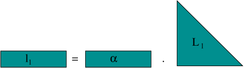
Figure 2: Recover of the coefficients of the first linear dependency

Now for the second block, the first linearly dependent vector $A^{d_{2}}v_{2}$ satisfies a relation of the type :

$$A^{d_{2}}v_{2}=\sum_{i=0}^{d_{2}-1}\beta_{i}A^{i}v_{2}+\sum_{i=0}^{d_{1}-1}\gamma_{i}A^{i}v_{1}$$

The vector of coefficients $\beta=[\beta_{i}]$ and $\gamma=[\gamma_{i}]$ can be obtained by solving the following system shown in figure 3.

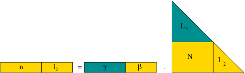
Figure 3: Recover of the coefficients of the second linear dependency

There only remains to build the Hessenberg polycyclic matrix from these vectors :

$$H=\left[\begin{array}[]{cccccccc}0&&&\alpha_{0}&&&&\gamma_{0}\\ 1&0&&\alpha_{1}&&&&\gamma_{1}\\ &\ddots&\ddots&\vdots&&&&\vdots\\ &&1&\alpha_{d_{1}-1}&&&&\gamma_{d_{1}-1}\\ &&&&0&&&\beta_{0}\\ &&&&1&0&&\beta_{1}\\ &&&&&\ddots&\ddots&\vdots\\ &&&&&&1&\beta_{d_{2}-1}\\ \end{array}\right].$$

This technique can be applied to every block of iterates. Therefore the Hessenberg polycyclic matrix can be recovered by as many triangular system resolutions as the number of blocks.

5.2 The main algorithm

We have seen in section 4 how to compute the matrix $T$ (simply $T=\left[\begin{array}[]{c|c}\overline{K}&P^{T}\left[\begin{array}[]{c}0\\ I_{n-r}\end{array}\right]\end{array}\right]$). Section 5.1 showed how to compute $H$. There only remains to show how to compute the matrices $X,Y$ and $B_{1}$ and we will be done.

We recall (from the proof of theorem 4.2) that

$$AT = \left[\begin{array}[]{c|c}AV&AP^{T}\left[\begin{matrix}0\\ I_{n-r}\end{matrix}\right]\end{array}\right]$$

$$= T\left[\begin{matrix}H&X\\ 0&Y\end{matrix}\right]$$

Then $X$ and $Y$ satisfy $T\left[\begin{matrix}X\\ Y\end{matrix}\right]=AP^{T}\left[\begin{matrix}0\\ I_{n-r}\end{matrix}\right]$. Let us write

$$A^{\prime}=PAP^{T}=\left[\begin{matrix}A^{\prime}_{11}&A^{\prime}_{12}\\ A^{\prime}_{21}&A^{\prime}_{22}\end{matrix}\right].$$

We have

$$T\left[\begin{matrix}X\\ Y\end{matrix}\right]=P^{T}A^{\prime}\left[\begin{matrix}0\\ I_{n-r}\end{matrix}\right]=P^{T}\left[\begin{matrix}A^{\prime}_{12}\\ A^{\prime}_{22}\end{matrix}\right]$$

Now

$$T=P^{T}\left[\begin{matrix}U_{1}^{T}&0\\ U_{2}^{T}&I_{n-r}\end{matrix}\right]\left[\begin{matrix}L^{T}&0\\ 0&I_{n-r}\end{matrix}\right],$$

therefore

$$\left[\begin{matrix}U_{1}^{T}&0\\ U_{2}&I_{n-r}\end{matrix}\right]\left[\begin{matrix}L^{T}&0\\ 0&I_{n-r}\end{matrix}\right]\left[\begin{matrix}X\\ Y\end{matrix}\right] = \left[\begin{matrix}A^{\prime}_{12}\\ A^{\prime}_{22}\end{matrix}\right]$$

$$\left[\begin{matrix}U_{1}^{T}&0\\ U_{2}^{T}&I_{n-r}\end{matrix}\right]\left[\begin{matrix}L^{T}X\\ Y\end{matrix}\right] = \left[\begin{matrix}A^{\prime}_{12}\\ A^{\prime}_{22}\end{matrix}\right]$$

And the system

$$\left\{\begin{array}[]{lcl}U_{1}^{T}L^{T}X&=&A^{\prime}_{12}\\ U_{2}^{T}L^{T}X+Y&=&A^{\prime}_{22}\end{array}\right.$$

has the following solution

$$\left\{\begin{array}[]{lcl}X&=&L^{-T}U_{1}^{-T}A^{\prime}_{12}\\ Y&=&A^{\prime}_{22}-U_{2}^{T}U_{1}^{-T}A^{\prime}_{12}\end{array}\right.$$

The computation of $B_{1}$ is straightforward from the equation $TB_{1}=B$ :

$$B_{1}=L^{-T}U_{1}^{-T}PB.$$

We are now able to write the algorithm.

Algorithm 1 Kalman form

0:  $A$ a $n\times n$ matrix over a field, $B$, a $n\times m$ matrix

0:  $r,T,H,X,Y,B_{1}$ as in theorem 4.1

1:  $(V,r)=\texttt{CompressedKrylovMatrix}(A,B)$

2:  if  (r=n) then

3:     return $(n,Id,A,\emptyset,\emptyset,B)$

4:  else

5:     $(L,[U_{1}U_{2}],P)=\text{LUP}(V^{T})$

6:     $T=\left[\begin{array}[]{c|c}V&P^{T}\left[\begin{array}[]{c}0\\ I_{n-r}\end{array}\right]\end{array}\right]$

7:     $B_{1}=L^{-T}U_{1}^{-T}PB$

8:     $A^{\prime}=PAP^{T}=\left[\begin{array}[]{cc}A^{\prime}_{11}&A^{\prime}_{12}\\ A^{\prime}_{21}&A^{\prime}_{22}\end{array}\right]$

9:     $X=L^{-T}U_{1}^{-T}A^{\prime}_{12}$

10:     $Y=A^{\prime}_{22}-U_{2}^{T}U_{1}^{-T}A^{\prime}_{12}$

11:     for all j do

12:        $m_{j}=l_{j}L^{-1}_{j}$ as explained in section 5.1

13:     end for

14:     Build the polycyclic matrix $H$ using the $m_{j}$ as shown in section 5.1.

15:     return $(r,T,H,X,Y,B_{1})$

16:  end if

Lastly, note that the LUP factorization of $V^{T}$ is already computed at the end of the call to CompressedKrylovMatrix. Thus, step 5 in algorithm 1 can be skipped.

5.3 LU-Krylov : a cubic variant

In [DPW05], we introduce an algorithm for the computation of the characteristic polynomial : LUK. Alike Keller-Gehrig’s algorithm, it is also based on the Krylov iterates of several vectors and relies as much as possible on matrix multiplication. But the krylov iterates are computed with matrix vector products, so as to avoid the $\text{log}n$ factor in the time complexity. As a consequence it is ${\cal O}(n^{3})$ algorithm, but we showed that it was faster in practice.

Algorithm 2 shows how to adapt this algorithm to the computation of the Kalman form. We expect this algorithm to be the more efficient in practice.

Algorithm 2 Kalman-LUK : Kalman-LU-Krylov

0:  $A$ a $n\times n$ matrix over a field, $B$, a $n\times m$ matrix

0:  $r,T,H,X,Y,B_{1}$ as in theorem 4.2

1:  $v=B_{1}$

2:  $\left\{\begin{array}[]{l}K=\left[\begin{matrix}v&Av&A^{2}v&\dots\end{matrix}\right]\\ (L,[U_{1}|U_{2}],P)=\text{{LUP}}(K^{T}),r_{1}=\mbox{rank}(K)\end{array}\right.$ {The matrix $K$ is computed on the fly : at most $2r_{1}$ columns are computed}

3:  $m=(m_{1},\dots,m_{r1})=L_{r_{1}+1}L_{1\dots r_{1}}^{-1}$

4:  $f=X^{r_{1}}-\sum_{i=1}^{r_{1}}{m_{i}X^{i-1}}$

5:  if  $(r_{1}=n)$  then

6:     return $(n,Id,A,\emptyset,\emptyset,B)$

7:  else

8:     $A^{\prime}=PAP^{T}=\left[\begin{array}[]{cc}A^{\prime}_{11}&A^{\prime}_{12}\\ A^{\prime}_{21}&A^{\prime}_{22}\end{array}\right]$ where $A^{\prime}_{11}$ is $r_{1}\times r_{1}$.

9:     $A_{R}=A^{\prime}_{22}-U_{2}^{T}U_{1}^{-T}A^{\prime}_{12}$

10:     $B^{\prime}=\left[\begin{matrix}L^{-T}&0\\ 0&I\end{matrix}\right]\left[\begin{matrix}U_{1}^{-T}&0\\ -U_{2}^{T}U_{1}^{-T}&I\end{matrix}\right]PB$

11:     Compute the permutation $Q$ s.t. $B^{\prime}Q=\left[\begin{matrix}*&*\\ 0&Z\end{matrix}\right]$ {$Z$ is $(n-r_{1})\times\mu$}

12:     if $(\mu=0)$ then

13:        $X=L^{-T}U_{1}^{-T}A^{\prime}_{12}$

14:        $Y=A_{R}$

15:        $T=\left[\begin{array}[]{c|c}K&P^{T}\left[\begin{matrix}0\\ I_{n-r_{1}}\end{matrix}\right]\end{array}\right]$

16:        return $(r_{1},T,C_{f},X,Y,X)$

17:     else

18:        $(r_{2},T^{(2)},H^{(2)},X^{(2)},Y^{(2)},B_{1}^{(2)})=\texttt{Kalman-LUK}(A_{R},Z)$

19:        $T=\left[\begin{array}[]{c|c}K&P^{T}\left[\begin{matrix}0\\ T^{(2)}\end{matrix}\right]\end{array}\right]$

20:        $J=L^{-T}U_{1}^{-T}A^{\prime}_{12}T^{(2)}=\left[\begin{matrix}J_{1}&J_{2}\end{matrix}\right]$ {$J_{1}$ is $r_{1}\times r_{2}$ and $J_{2}$, $r_{1}\times(n-r_{1}-r_{2})$}

21:        $H=\left[\begin{matrix}C_{f}&J_{1}\\ 0&H^{(2)}\end{matrix}\right]$

22:        $X=\left[\begin{matrix}J_{2}\\ X^{(2)}\end{matrix}\right]$

23:        return $(r_{1}+r_{2},T,H,X,Y^{(2)},B_{1})$

24:     end if

25:  end if

References

[CBS97]
Michael Clausen, Peter Burgisser, Mohammad A. Shokrollahi.
Algebraic Complexity Theory.
1997.
[DPW05]
Jean-Guillaume Dumas, Clément Pernet, Zhendong Wan.
Efficient computation of the characteristic polynomial.
Patrz Kauers [Kau05].
[DR05]
Jean-Guillaume Dumas, Aude Rondepierre.
Algorithms for symbolic/numeric control of affine dynamical system.
Patrz Kauers [Kau05].
[IMH82]
Oscar H. Ibarra, Shlomo Moran, Roger Hui.
A generalization of the fast LUP matrix decomposition algorithm and
applications.
Journal of Algorithms, 3(1):45–56, Marzec 1982.
[Kal61]
R.E. Kalman.
Canonical structure of linear dynamical systems.
Proceedings of the National Academy of Sciences, strony
596–600, 1961.
[Kau05]
Manuel Kauers, redaktor.
ISSAC’2005. Proceedings of the 2005 International Symposium on
Symbolic and Algebraic Computation, Beijing, China. ACM Press, New York,
Lipiec 2005.
[KG85]
Walter Keller-Gehrig.
Fast algorithms for the characteristic polynomial.
Theoretical computer science, 36:309–317, 1985.