On relating CTL to Datalog

Abstract

CTL is the dominant temporal specification language in practice mainly due to the fact that it admits model checking in linear time. Logic programming and the database query language Datalog are often used as an implementation platform for logic languages. In this paper we present the exact relation between CTL and Datalog and moreover we build on this relation and known efficient algorithms for CTL to obtain efficient algorithms for fragments of stratified Datalog. The contributions of this paper are: a) We embed CTL into STD which is a proper fragment of stratified Datalog. Moreover we show that STD expresses exactly CTL – we prove that by embedding STD into CTL. Both embeddings are linear. b) CTL can also be embedded to fragments of Datalog without negation. We define a fragment of Datalog with the successor build-in predicate that we call TDS and we embed CTL into TDS in linear time. We build on the above relations to answer open problems of stratified Datalog. We prove that query evaluation is linear and that containment and satisfiability problems are both decidable. The results presented in this paper are the first for fragments of stratified Datalog that are more general than those containing only unary EDBs.

1 Introduction

Temporal logics are modal logics used for the description and specification of the temporal ordering of events [Eme90]. Pnueli was the first to notice that temporal logics could be particularly useful for the specification and verification of reactive systems [Pnu77, Pnu81]. In defining temporal logics, there are two possible views regarding the flow of time. One is that of linear time; at each moment there is only one possible future (Linear Temporal Logic-LTL). The other is that of branching time (tree-like nature); at each moment time may follow different paths which represent different possible futures [EH86, Lam80]. The most prominent examples of the latter are CTL (Computational Tree Logic), CTL^⋆ (Full Branching Time Logic), and $\mu$-calculus.

Deciding whether a system meets a specification expressed in a language of temporal logic is called model checking. Model checking is decidable when the system is abstracted as a finite directed labeled graph and the specification is expressed in a propositional temporal language. Model checking has been widely used for verifying the correctness of, or finding design errors in many real-life systems [CW96]. Through the 1990s, CTL has become the dominant temporal specification language for industrial use [Var01, CGL93] mostly due to its balance of expressive power and linear model checking complexity. SMV [McM93], the first symbolic model checker (CTL -based), and its follower VIS [BHS⁺96] (also CTL -based), presented phenomenal success and serve as the basis for many industrial model checkers.

The introduction of Datalog [Ull88] represented a major breakthrough in the design of declarative, logic-oriented database languages due to Datalog’s ability to express recursive queries. Datalog is a rule-based language that has simple and elegant semantics based on the notion of minimal model or least fixpoint. This leads to an operational semantics that can be implemented efficiently, as demonstrated by a number of prototypes of deductive database systems [NT89, RSS92, ELM⁺97]. Datalog queries are computed in polynomial time; however, it has been shown that Datalog only captures a proper subset of monotonic polynomial-time queries [ACY91].

In order to express queries of practical interest, negation is allowed in the bodies of Datalog rules. Of particular interest is stratified negation, which avoids the semantic and implementation problems connected with the unrestricted use of nonmonotonic constructs in recursive definitions. In stratified Datalog [ABW88, Ull88, CH85] negation is allowed in any predicate under the constraint that negated predicates are computed in previous strata. Simple, intuitive semantics leading to efficient implementation exists for stratified Datalog. Unfortunately, as shown in [Kol91], this language has a limited expressive power as it can only express a proper subset of fixpoint queries.

We have three major contributions in this paper. The first contribution is the definition of a fragment of stratified Datalog (the class STD) which has the exact expressive power as CTL (Theorem 4.1). We prove that by establishing a linear embedding from STD into CTL and vice versa. This is the first time that a fragment of stratified Datalog is identified which expresses exactly CTL. The definition of this fragment is simple and natural (see Subsection 4.1).

For our second contribution, we build on the above result to solve open problems of stratified Datalog. More specifically we prove that: a) query evaluation for STD is linear by reducing it to the model checking problem of CTL and b) both satisfiability and containment problems are decidable for STD programs by reduction to the validity problem of CTL. This is the first result that proves decidability of containment for a fragment of stratified Datalog which uses EDB (Extensional Database) relations other than unary and hence it has not a limited number of nontrivial strata. Checking containment of queries, i.e., verifying whether one query yields a subset of the result of the other, has been the subject of research last decades. Query containment is crucial in many contexts such as query optimization, query reformulation, knowledge-base verification, information integration, integrity checking and cooperative answering. Table 1 presents all known results on query containment for stratified Datalog including the results we obtain here.

We also consider a fragment of a variant of Datalog without negation. We define the class TDS which is a fragment of Datalog_Succ and establish a linear embedding from CTL to TDS. Datalog_Succ is Datalog enhanced with the build-in successor predicate and allows negation only in the EDB predicates. The successor predicate is needed to express the universal quantifier which in stratified Datalog can be captured by using the full power of negation. Note that we use the conventional semantics of Datalog and this constitutes a contribution relatively to previous works [GFAA03]. This is the third contribution.

	Stratified	STD	Stratified negation
	negation	(Stratified negation with unary	with unary
		+ 1 binary EDB predicates)	EDB predicates
Containment	undecidable	EXPTIME–complete [Section 6]	decidable
			[LMSS93, HMSS01]
Equivalence	undecidable	EXPTIME–complete [Section 6]	decidable
			[LMSS93, HMSS01]
Satisfiability	undecidable	EXPTIME–complete [Section 6]	decidable
			[LMSS93, HMSS01]
Evaluation	polynomial	linear [Section 6]	linear [Section 6]

Table 1: Results on fragments of Stratified Datalog

1.1 Motivating Examples

The following three examples illustrate some of the subtle points of the translation of a CTL formula into stratified Datalog and they are presented in order of increasing complexity. The subtleties in the case of Datalog_Succ are of similar nature. In all examples, we consider a Kripke structure $\mathcal{K}$, which is given by: a set of states $W$, the transition relation $R$ on the states, and atomic propositions assigned to the states.

Example 1.1

This is the first motivating example for our translation techniques. Consider the CTL formula: $\varphi\equiv\mathbf{E}{\bigcirc}p$. It says that, there exists a path starting from a state $s_{0}$ such that the next state on this path is assigned the atomic proposition $p$. We may view the Kripke structure as a database $D$ with unary EDB predicates for the atomic propositions $($here EDB predicate $P$ is associated to $p$$)$ and a binary EDB predicate $R$ for the transition relation. Now the following Datalog program says that if $s_{0}$ is computed in the answers of the query predicate $G$, then there exists a path in $D$ starting from $s_{0}$ which in one transition step reaches a state where $P$ is true.

$\left\{\begin{array}[]{l}G(x)\longleftarrow R(x,y),G_{1}(y)\\ G_{1}(x)\longleftarrow P(x)\\ \end{array}\right.$

$\blacktriangle$

Whereas this is not a recursive program, when the formula contains the “until” modality, recursion is needed as is the case in the example that follows.

Example 1.2

Consider now the somewhat more complex formula $\varphi\equiv$ $\mathbf{E}{\bigcirc}p$ $\wedge$ $\mathbf{E}(q\mathbf{U}t)$. The Datalog query that expresses this formula is the following.

$\left\{\begin{array}[]{l}G(x)\longleftarrow G_{1}(x),G_{2}(x)\\ G_{1}(x)\longleftarrow R(x,y),G_{3}(y)\\ G_{3}(x)\longleftarrow P(x)\\ G_{2}(x)\longleftarrow G_{4}(x)\\ G_{2}(x)\longleftarrow G_{5}(x),R(x,y),G_{2}(y)\\ G_{4}(x)\longleftarrow T(x)\\ G_{5}(x)\longleftarrow Q(x)\\ \end{array}\right.$

This Datalog query expresses what the CTL formula says, i.e., there exists a path starting from a state $s_{0}$ that is assigned $p$ on its next state and there is also a path $($different or the same$)$ such that it is assigned $q$ along all its states up until it gets to a state that is assigned $t$. The second and third rules express the CTL formula $\mathbf{E}{\bigcirc}p$, the four last rules express the CTL formula $\mathbf{E}(q\mathbf{U}t)$ and the first rule asserts the conjunction of $\mathbf{E}{\bigcirc}p$ and $\mathbf{E}(q\mathbf{U}t)$. $\blacktriangle$

Now, there is a more complicated recursive case which requires a recursive predicate with two arguments and this is demonstrated in the third example.

Example 1.3

Consider the CTL formula $\mathbf{E}\square p$ which can also be written as $\mathbf{E}(\bot\mathbf{\widetilde{U}}p)$. This formula says that there is an infinite path from a state $s_{0}$ so that $p$ holds in all the states of the path. The existence of an infinite path on a finite Kripke structure is equivalent to the existence of a cycle. The following Datalog program expresses exactly this formula. In this program the rules with head predicate $W$ are ancillary, they just say that $x$ is an element of the domain $($the EDB predicates $P_{i},0\leq i\leq n$, correspond to the atomic propositions$)$. They are used to obtain safe rules and to express true and false – note that the second rule never fires, hence $G_{2}$ expresses false and $G_{1}$ expresses true. Thus the rules that express the essential meaning of the formula are 3–8.

$\left\{\begin{array}[]{l}G_{1}(x)\longleftarrow W(x)\\ G_{2}(x)\longleftarrow W(x),\neg G_{1}(x)\\ G_{3}(x)\longleftarrow P(x)\\ G(x)\longleftarrow G_{2}(x),G_{3}(x)\\ G(x)\longleftarrow B(x,x)\\ G(x)\longleftarrow G_{3}(x),R(x,y),G(y)\\ B(x,y)\longleftarrow G_{3}(x),R(x,y),G_{3}(y)\\ B(x,y)\longleftarrow G_{3}(x),R(x,u),B(u,y)\\ W(x)\longleftarrow R(x,y)\\ W(x)\longleftarrow R(y,x)\\ W(x)\longleftarrow P_{0}(x)\\ \dots\\ W(x)\longleftarrow P_{n}(x)\\ \end{array}\right.$

The two rules $($7th and 8th$)$ that compute $B$ $($combined with the third rule$)$ actually compute the transitive closure of $R$ over states where $P$ is true. The fifth rule says that the formula holds if there is a cycle starting from state $s_{0}$ with $P$ assigned to all its states. The sixth rule says that the formula holds if there is a path which is followed by a cycle from a state $s_{0}$ with $P$ assigned to all their states. $\blacktriangle$

1.2 Technical Challenges

The examples illustrated the part of our contribution that translates a CTL formula to a Datalog query. However there are a few technical challenges that do not show on these examples: 1) By a straightforward translation some Datalog rules might not be safe (i.e., they may have variables that do not occur in nonnegated body subgoals). Thus we introduce a number of rules which essentially define the domain by an IDB (Intentional Database) predicate which is used in rules for safety – this shows a little in Example 1.3. 2) Trying to identify a fragment of Datalog with exactly the same expressive power as CTL and use this fact to prove results for this fragment, we have to deal with the fact that CTL is interpreted over infinite paths. This means that finite Kripke structures over which we interpret CTL have to be total on the binary relation $R$. Relational databases however over which Datalog programs are interpreted do not have any constraints, i.e., the input could be any structure of the given schema. A solution to this kind of problem that is suggested in the literature [Eme90] is to add a self loop in those nodes that do not have a successor in $R$. We adopt a similar solution only that we encompass it in the definitions of the Datalog fragment we define, allowing thus for any input database to be captured. The example that follows explains further this point.

Example 1.4

Consider the following Datalog program

$\left\{\begin{array}[]{l}A(x)\longleftarrow R(x,y)\\ G(x)\longleftarrow\neg A(x),P(x)\\ G(x)\longleftarrow R(x,y),P(y)\end{array}\right.$

It is easy to see that it returns the same answer on any pair of databases which only differ in adding self loops in $R$ on nodes that do not have a successor in $R$. $\blacktriangle$

Finally, our results go through because CTL has the bounded model property which means that if there is a model for a CTL formula then there is a finite model. Since in CTL infinite models are also assumed, in order to carry over results to Datalog where finite input is assumed, we make use of this property.

The rest of the paper is organized as follows. Sections 2 and 3 are preliminary sections that define formally CTL (Section 2), Datalog, Datalog_Succ and stratified Datalog (Section 3). Section 4 presents the formalism of our translation, discusses the notion of equivalence between CTL formulae and Datalog queries and defines the class of Stratified Temporal Datalog (STD) programs which is a fragment of stratified Datalog. The embedding from CTL to STD is also presented in Section 4. Section 5 gives the embedding from STD to CTL which is not straightforward so a discussion on the technical challenges of this embedding is also included. In Section 6 we prove that query evaluation for STD programs is linear and that checking containment and satisfiability is decidable. The embedding of CTL into Datalog_Succ is presented in Section 7. Finally, Section 8 shows how the present work can be extended to infinite structures and discusses possible future research directions. The proof of Theorem 7.1 is presented in the Appendix.

1.3 Related Work

Model checking is closely related to database query evaluation. The idea is based on the principle that Kripke structures can be viewed as relational databases [IV97]. One effective approach for efficiently implementing model checking is based on the translation of temporal formulae into automata and has become an intensive research area [WVS83, VW86, VW94]. Another approach consists in translating temporal logics to Logic Programming [Llo87]. Logic Programming has been successfully used as an implementation platform for verification systems such as model checkers. Translations of temporal logics such as CTL or $\mu$-calculus into logic programming can be found in [RRR⁺97, CDD⁺98, CP98]. [CDD⁺98] presents the LMC project which uses XSB, a tabled logic programming system that extends Prolog-style SLD resolution with tabled resolution.

The database query language Datalog has inspired work in [GGV02], where the language Datalog LITE is introduced. Datalog LITE is a variant of Datalog that uses stratified negation, restricted variable occurrences and a limited form of universal quantification in rule bodies. Datalog LITE is shown to encompass CTL and the alternation-free $\mu$-calculus. Research on model checking in the modal $\mu$-calculus is pursued in [ZSS94] where the connection between modal $\mu$-calculus and Datalog is observed. This is used to derive results about the parallel computational complexity of this fragment of modal $\mu$-calculus.

In previous work [GFAA03] we showed that the model checking problem for CTL can be reduced to the query evaluation problem for fragments of Datalog. In more detail, [GFAA03] presents a direct and modular translation from the temporal logics CTL, ETL, FCTL (CTL extended with the ability to express fairness) and the modal $\mu$-calculus to Monadic inf-Datalog with built-in predicates. It is called inf-Datalog because the semantics differ from the conventional Datalog least fixed point semantics, in that some recursive rules (corresponding to least fixed points) are allowed to unfold only finitely many times, whereas others (corresponding to greatest fixed points) are allowed to unfold infinitely many times. The work in [AAP⁺03], which is a preliminary version of some of the results presented here, embeds CTL into a fragment of Datalog_Succ.

We know that CTL can be embedded into Transitive Closure logic [IV97] and into alternation- free $\mu$–calculus [Eme96]. In [GGV02] the authors observe that CTL can be embedded into stratified Datalog. In this paper it is the first time that the exact fragment of stratified Datalog with the same expressive power with CTL has been identified.

Concerning containment of queries the majority of research refers to CQs. However there are important results concerning also Datalog programs. In [CGKV88] it was pointed out that query containment for monadic Datalog is decidable. The work in [Sag88] shows that checking containment of nonrecursive Datalog queries in Datalog queries is decidable in exponential time. In [CV97] it is shown that containment of Datalog queries in non-recursive Datalog is decidable in triply exponential time, whereas when the non-recursive query is represented as a union of CQs, the complexity is doubly exponential. In [LMSS93, HMSS01] authors proved that equivalence of stratified Datalog programs is decidable but only for programs with unary EDB predicates. Our results are the first that encompass also programs that contain binary EDB predicates.

2 CTL

2.1 Syntax and Semantics of CTL

Temporal logics are classified as linear or branching according to the way they perceive the nature of time. In linear temporal logics every moment has a unique future (successor), whereas in branching temporal logics every moment may have more than one possible futures. Branching temporal logic formulae are interpreted over infinite trees or graphs that can be unwound into infinite trees. Such a structure can be thought of as describing all the possible computations of a nondeterministic program (branches stand for nondeterministic choices). Note that a time step is usually identified with a computation step (e.g., a clock tick in a synchronous design). The future is considered to be the reflexive future, it includes the present, and time is considered to unfold in discrete steps.

CTL (Computational Tree Logic) [CE81, EC82] is a branching temporal logic that uses the path quantifiers $\mathbf{E}$, meaning “there exists a path”, and $\mathbf{A}$, meaning “for all paths”. A path is an infinite sequence of states such that each state and its successor are related by the transition relation. The syntax of CTL formulae uses temporal operators as well. For instance, to assert that “property $\varphi$ is always true on every path” or that “there is a path on which property $\psi_{1}$ is true until $\psi_{2}$ becomes true” one writes $\mathbf{A}\Box\varphi$ and $\mathbf{E}(\psi_{1}\mathbf{U}\psi_{2})$, respectively, where $\Box$ and $\mathbf{U}$ are temporal operators. Various temporal operators are listed in the literature as part of the CTL syntax. However the operators ${\bigcirc}$ and $\mathbf{U}$ form a complete set from which we can express all other operators. We give the syntax of CTL in terms of these two temporal operators and later we also use the operator $\mathbf{\widetilde{U}}$, which facilitates our translations.

The syntax of CTL dictates that each usage of a temporal operator must be preceded by a path quantifier. These pairs consisting of the path quantifier and the temporal operator can be nested arbitrarily, but must have at their core a purely propositional formula. In the remaining of the paper $AP$ denotes the set of atomic propositions: $\{p_{0},p_{1},p_{2},\ldots\}$ from which CTL formulae are built. We proceed to the formal definition of the syntax of CTL.

S₁.  Atomic propositions, $\top$ and $\bot$ are CTL formulae.
S₂.  If $\varphi,\psi$ are CTL formulae then so are $\neg\varphi$, $\varphi\wedge\psi$, $\varphi\vee\psi$.
S₃.  If $\varphi,\psi$ are CTL formulae then $\mathbf{E}{\bigcirc}\varphi$, $\mathbf{A}{\bigcirc}\varphi$, $\mathbf{E}(\varphi\mathbf{U}\psi)$, $\mathbf{A}(\varphi\mathbf{U}\psi)$ are CTL formulae.

The semantics of CTL is defined over temporal Kripke structures. A temporal Kripke structure $\mathcal{K}$ is a directed labeled graph with node set $W$, arc set $R$ and labeling function $V$. $\mathcal{K}$ need not be a tree; however, it can be turned into an infinite labeled tree if unwound from a $s_{0}$ (see [Eme90] and [Var97] for details). Below we give the definition of temporal Kripke structures.

Definition 2.1

Let $AP$ be the set of atomic propositions. A temporal Kripke structure $\mathcal{K}$ for $AP$ is a tuple $\langle W,R$, $V\rangle$, where:

• $W$ is the set of states,

• $R\subseteq W\times W$ is the total accessibility relation, and

• $V:W\longrightarrow 2^{AP}$ is the valuation that determines which atomic propositions are true at each state.

A finite Kripke structure $\mathcal{K}$ is a Kripke structure $\langle W,R,V\rangle$ with finite $W$.  

In Kripke structures the set of states $W$ can be infinite. $W$ as defined in Definition 2.1 may be of any cardinality. In this paper we are interested in relational databases, where the universe $W$ is finite. Hence, our Kripke structures are finite. In CTL we are dealing with infinite computation paths, which means that in order for the accessibility relation $R$ to be meaningful, $R$ must be total ([KVW00]):

$$\forall x\exists y\ R(x,y)$$ (1)

Definition 2.2

A path $\pi$ of $\mathcal{K}$ is an infinite sequence $s_{0},s_{1},s_{2},\ldots$ of states of $W$, such that $R(s_{i},s_{i+1})$, $i\geq 0$. We also use the notational convention $\pi^{i}=s_{i},s_{i+1},s_{i+2},\ldots$ .    

The notation $\mathcal{K},s\models\varphi$ means that “the formula $\varphi$ holds at state $s$ of $\mathcal{K}$”. The meaning of $\models$ is formally defined as follows:

Definition 2.3

• $\models\top$ and  $\not\models\bot$

• $\mathcal{K},s\models p\Longleftrightarrow p\in V(s)$, for an atomic proposition $p\in AP$

• $\mathcal{K},s\models\neg\varphi\Longleftrightarrow\mathcal{K},s\not\models\varphi$

• $\mathcal{K},s\models\varphi\vee\psi\Longleftrightarrow\mathcal{K},s\models\varphi$ or $\mathcal{K},s\models\psi$

• $\mathcal{K},s\models\varphi\wedge\psi\Longleftrightarrow\mathcal{K},s\models\varphi$ and $\mathcal{K},s\models\psi$

• $\mathcal{K},s\models\mathbf{E}\varphi\Longleftrightarrow$ there exists a path $\pi=s_{0},s_{1},\ldots$, with initial state $s=s_{0}$, such that $\mathcal{K},\pi\models\varphi$

• $\mathcal{K},s\models\mathbf{A}\varphi\Longleftrightarrow$ for every path $\pi=s_{0},s_{1},\ldots$, with initial state $s=s_{0}$ it holds that $\mathcal{K},\pi\models\varphi$

• $\mathcal{K},\pi\models{\bigcirc}\varphi\Longleftrightarrow\mathcal{K},\pi^{1}\models\varphi$

• $\mathcal{K},\pi\models\varphi\mathbf{U}\psi\Longleftrightarrow$ there exists $i\geq 0$ such that $\mathcal{K},\pi^{i}\models\psi$ and for all $j,\ 0\leq j<i,$ $\mathcal{K},\pi^{j}\models\varphi$

• $\mathcal{K},\pi\models\varphi\mathbf{\widetilde{U}}\psi\Longleftrightarrow$ for all $i\geq 0$ such that $\mathcal{K},\pi^{i}\not\models\psi$ there exists $j,\ 0\leq j<i,$ such that $\mathcal{K},\pi^{j}\models\varphi$  

A CTL state formula $\varphi$ is satisfiable if there exists a Kripke structure $\mathcal{K}=\langle W,R,V\rangle$ such that $\mathcal{K},s\models\varphi$, for some $s\in W$. In this case $\mathcal{K}$ is a model of $\varphi$. If $\mathcal{K},s\models\varphi$ for every $s\in W$, then $\varphi$ is true in $\mathcal{K}$, denoted $\mathcal{K}\models\varphi$. If $\mathcal{K}\models\varphi$ for every $\mathcal{K}$, then $\varphi$ is valid, denoted $\models\varphi$. If $\mathcal{K}\models\varphi$ for every finite $\mathcal{K}$, we say that $\varphi$ is valid with respect to the class of finite Kripke structures, denoted $\models_{f}\varphi$.

The truth set of a CTL formula $\varphi$ with respect to a Kripke structure $\mathcal{K}$ is the set of states of $\mathcal{K}$ at which $\varphi$ is true. We define formally the truth set as follows:

Definition 2.4

$($Truth set$)$ Given a CTL formula $\varphi$ and a Kripke structure $\mathcal{K}=\langle W,R,V\rangle$, the truth set of $\varphi$ with respect to $\mathcal{K}$, denoted $\varphi[\mathcal{K}]$, is $\{s\in W\ |\ \mathcal{K},s\models\varphi\}$.  

2.2 Normal Forms

CTL formulae can be transformed in two normal forms: existential normal form and positive normal form. The translations we give in Sections 4 and 7 cover each of these two syntactic variations of CTL.

2.2.1 Existential Normal Form

In existential normal form negation is allowed to appear in front of CTL formulae. The universal path quantifier $\mathbf{A}$ is cast in terms of its dual existential path quantifier $\mathbf{E}$ using negation and the temporal operator $\mathbf{\widetilde{U}}$: $\mathbf{A}(\psi_{1}\mathbf{U}\psi_{2})$ becomes $\neg\mathbf{E}(\neg\psi_{1}\mathbf{\widetilde{U}}\neg\psi_{2})$. The $\mathbf{\widetilde{U}}$ operator was initially introduced in [Var98, KVW00] as the dual operator of $\mathbf{U}$. One can think of $\mathbf{E}(\psi_{1}\mathbf{\widetilde{U}}\psi_{2})$ as saying that there exists a path on which:
(1) either $\psi_{2}$ always holds, or
(2) the first occurrence of $\neg\psi_{2}$ is strictly preceded by an occurrence of $\psi_{1}$.

In general, every CTL formula can be written in existential normal form using negation, the temporal operators ${\bigcirc}$, $\mathbf{U}$, $\mathbf{\widetilde{U}}$ and the existential path quantifier $\mathbf{E}$ (without the universal path quantifier $\mathbf{A}$). The syntax in this case is given by rules S${}_{1}^{\prime}$-S${}_{3}^{\prime}$ and Proposition 2.1 states formally the equivalence of the two forms.

S${}_{1}^{\prime}$.  Atomic propositions and $\top$ are CTL formulae.
S${}_{2}^{\prime}$.  If $\varphi,\psi$ are CTL formulae then so are $\neg\varphi$, $\varphi\wedge\psi$.
S${}_{3}^{\prime}$.  If $\varphi,\psi$ are CTL formulae then $\mathbf{E}{\bigcirc}\varphi$, $\mathbf{E}(\varphi\mathbf{U}\psi)$ and $\mathbf{E}(\varphi\mathbf{\widetilde{U}}\psi)$ are CTL formulae.

Proposition 2.1

Every CTL formula $\varphi$ can be transformed into a CTL formula $\varphi^{\prime}$ in existential normal form such that $\mathcal{K},s\models\varphi$  iff  $\mathcal{K},s\models\varphi^{\prime}$ for every $\mathcal{K}=\langle W,R,V\rangle$ and every $s\in W$.

Proof
The universal path quantifier $\mathbf{A}$ is expressed as follows: $\mathbf{A}{\bigcirc}\psi$ is rewritten as $\neg\mathbf{E}{\bigcirc}\neg\psi$, $\mathbf{A}(\psi_{1}\mathbf{U}\psi_{2})$ as $\neg\mathbf{E}(\neg\psi_{1}\mathbf{\widetilde{U}}\neg\psi_{2})$ and $\mathbf{A}(\psi_{1}\mathbf{\widetilde{U}}\psi_{2})$ as $\neg\mathbf{E}(\neg\psi_{1}\mathbf{U}\neg\psi_{2})$. The correctness of these transformations follows immediately from Definition 2.3. Also $\bot$ can be viewed as an abbreviation of $\neg\top$. $\dashv$

The translation presented in Section 4 translates CTL formulae in existential normal form into stratified Datalog. As the universal quantifier is not used, stratified Datalog expresses nicely CTL formulae.

2.2.2 Positive Normal Form [Var98]

Every CTL formula can be equivalently written in positive normal form where negation is applied only on atomic propositions. However, to compensate for the loss of full negation we need to use also the temporal operator $\mathbf{\widetilde{U}}$. Every CTL formula can be written in positive normal form using negation applied only on atomic propositions, the temporal operators ${\bigcirc}$, $\mathbf{U}$ and $\mathbf{\widetilde{U}}$ and both existential $\mathbf{E}$ and universal $\mathbf{A}$ path quantifiers. This is achieved by pushing negations inward as far as possible using De Morgan’s laws and dualities of path quantifiers and temporal operators. The syntax of CTL in this case is given by rules S${}_{1}^{\prime\prime}$-S${}_{3}^{\prime\prime}$.

S${}_{1}^{\prime\prime}$.  Atomic propositions, $\top$ and their negation are CTL formulae.
S${}_{2}^{\prime\prime}$.  If $\varphi,\psi$ are CTL formulae then so are $\varphi\wedge\psi$, $\varphi\vee\psi$.
S${}_{3}^{\prime\prime}$.  If $\varphi,\psi$ are CTL formulae then $\mathbf{E}{\bigcirc}\varphi$, $\mathbf{A}{\bigcirc}\varphi$, $\mathbf{E}(\varphi\mathbf{U}\psi)$, $\mathbf{A}(\varphi\mathbf{U}\psi)$, $\mathbf{E}(\varphi\mathbf{\widetilde{U}}\psi)$ and $\mathbf{A}(\varphi\mathbf{\widetilde{U}}\psi)$ are CTL formulae.

Proposition 2.2

Every CTL formula $\varphi$ can be transformed into a CTL formula $\varphi^{\prime}$ in positive normal form such that $\mathcal{K},s\models\varphi$  iff  $\mathcal{K},s\models\varphi^{\prime}$ for every $\mathcal{K}=\langle W,R,V\rangle$ and every $s\in W$.

Proof
The proof can be found in [Var98]. $\dashv$

The translation in Section 7 considers CTL formulae in positive normal form and translates them into Datalog enhanced with the $Succ$ operator; the latter is needed to express the universal path quantifier. It turns out that in this translation there is no need for negation in recursively defined predicates. Table 2 presents the two normal forms in which a CTL formula can be written in, and the corresponding fragments of Datalog used for the translation.

Translation	CTL Normal Form	Datalog
[Section 4]	Existential Normal Form	Stratified Datalog
[Section 7]	Positive Normal Form	Datalog + $Succ$

Table 2: Normal forms vs. Datalog fragments

2.3 Model Checking and Complexity

Model checking is the problem of verifying the conformance of a finite state system to a certain behavior, i.e., verifying that the labeled transition graph satisfies (is a model of) the formula that specifies the behavior. Hence, given a labeled transition graph $\mathcal{K}$, a state $s$ and a temporal formula $\varphi$, the model checking problem for $\mathcal{K}$ and $\varphi$ is to decide whether $\mathcal{K},s\models\varphi$. The size of the labeled transition system $\mathcal{K}$, denoted $|\mathcal{K}|$, is taken to be $|W|+|R|$ and the size of the formula $\varphi$, denoted $|\varphi|$, is the number of symbols in $\varphi$.

For CTL formulae the model checking problem is known to be P–hard [Sch03], something that makes highly improbable the development of efficient parallel algorithms. However, there exist efficient algorithms that solve it in $O(|\mathcal{K}||\varphi|)$ time [CES86]. It is insightful to examine how the two parameters $|\mathcal{K}|$ and $|\varphi|$ affect the complexity. This can be done by introducing the following two complexity measures for the model checking problem [VW86]:

• data complexity, which assumes a fixed formula and variable Kripke structures, and

• program or formula complexity, which refers to variable formulae over a fixed Kripke structure.

CTL model checking is NLOGSPACE–complete with respect to data complexity and its formula complexity is in $O(\log|\varphi|)$ space [Sch03]. Another important problem for CTL is the validity problem, that is deciding whether a formula $\varphi$ is valid or not. This problem is much harder; it has been shown to be EXPTIME -complete [Var97]. The following two theorems state known results of CTL on which we built in Section 6 to argue about stratified Datalog.

Theorem 2.1

$($Validity$)$ [Var97] The validity problem for CTL is EXPTIME–complete.

CTL exhibits another important property, namely the bounded model property: if a formula $\varphi$ is satisfiable, then $\varphi$ is satisfiable in a structure of bounded cardinality.

Theorem 2.2

$($Bounded Model Property$)$ [Eme90] If a CTL formula $\varphi$ has a model, then $\varphi$ has a model with at most $2^{|\varphi|}$ states.

3 Datalog

Datalog [Ull88] is a query language for relational databases. An atom is an expression of the form $E(x_{1},\ldots,x_{r})$, where $E$ is a predicate symbol and $x_{1},\ldots,x_{r}$ are either variables or constants. A ground fact (or ground atom) is an atom of the form $E(c_{1},\ldots,c_{r})$, where $c_{1},\ldots,c_{r}$ are constants. From a logic perspective, a relation $\widehat{E}$ corresponding to predicate symbol $E$ is just a finite set of ground facts of $E$ and a relational database $D$ is a finite collection of relations. To simplify notation, in the rest of this paper we use the same symbol for the relation and the predicate symbol; which one is meant will be made clear by the context.

Definition 3.1

[DEGV01] A database schema $\mathfrak{D}$ is an ordered tuple $\langle W,E_{1}$, …, $E_{n}\rangle$, where $W$ is the domain of the schema and $E_{1},\ldots,E_{n}$ are predicate symbols, each with its associated arity.

Given a database schema $\mathfrak{D}$, the set of all ground facts formed from $E_{1},\ldots,E_{n}$ using as constants the elements of $W$ is denoted $\mathcal{H}_{B}(W)$. A database $D$ over $\mathfrak{D}$ is a finite subset of $\mathcal{H}_{B}(W)$; in this case, we say that $\mathfrak{D}$ is the underlying schema of $D$. The size of a database $D$, denoted $|D|$, is the number of ground facts in $D$.  

Definition 3.2

A Datalog program $\Pi$ is a finite set of function-free Horn clauses, called rules, of the form:

$G(x_{1},\ldots,x_{n})\longleftarrow B_{1}(y_{1,1},\ldots,y_{1,n_{1}}),\ldots,B_{k}(y_{k,1},\ldots,y_{k,n_{k}})$

where:
- $x_{1},\ldots,x_{n}$ are variables,
- $y_{i,j}$’s are either variables or constants,
- $G(x_{1},\ldots,x_{n})$ is a predicate atom, called the head of the rule, and
- $B_{1}(y_{1,1},\ldots,y_{1,n_{1}})$, …, $B_{k}(y_{k,1},\ldots,y_{k,n_{k}})$ are atoms that comprise the body of the rule.  

Predicates that appear in the head of some rule are called IDB (Intensional Database) predicates , while predicates that appear only in the bodies of the rules are called EDB (Extensional Database) predicates. Each Datalog program $\Pi$ is associated with an ordered pair of database schemas $(\mathfrak{D}_{i},\mathfrak{D}_{o})$, called the input-output schema, as follows: $\mathfrak{D}_{i}$ and $\mathfrak{D}_{o}$ have the same domain and contain exactly the EDB and IDB predicates of $\Pi$, respectively. Given a database $D$ over $\mathfrak{D}_{i}$ the set of ground facts for the IDB predicates, which can be deduced from $D$ by applications of the rules in $\Pi$, is the output database $D^{\prime}$ (over $\mathfrak{D}_{o}$), denoted $\Pi(D)$. Databases over $\mathfrak{D}_{i}$ are mapped to databases over $\mathfrak{D}_{o}$ via $\Pi$.

Definition 3.3

Given a Datalog program $\Pi$ we distinguish an IDB predicate $G$ and call it the goal $($or query$)$ predicate of $\Pi$. Let $D$ be an input database; The query evaluation problem for $G$ and $D$ is to compute the set of ground facts of $G$ in $\Pi(D)$, denoted $G_{\Pi}(D)$.  

The dependency graph of a Datalog program is a directed graph with nodes the set of IDB predicates of the program; there is an arc from predicate $B$ to predicate $G$ if there is a rule with head an instance of $G$ and at least one occurrence of $B$ in its body. The size of a rule $r$, denoted $|r|$, is the number of symbols appearing in $r$. Given a Datalog program $\Pi=\left\{\begin{array}[]{l}r_{n}\\ \ldots\\ r_{0}\\ \end{array}\right.$, the size of $\Pi$, denoted $|\Pi|$, is $|r_{0}|+\ldots+|r_{n}|$.

Stratified Datalog

Intuitively, stratified Datalog is a fragment of Datalog with negation allowed in any predicate under the constraint that negated predicates are computed in previous strata. Each head predicate of $\Pi$ is a head predicate in precisely one stratum $\Pi_{i}$ and appears only in the body of rules of higher strata $\Pi_{j}$ ($j>i$) [GGV02]. In particular this means that:

1. If $G$ is the head predicate of a rule that contains a negated $B$ as a subgoal, then $B$ is in a lower stratum than $G$.

2. If $G$ is the head predicate of a rule that contains a non negated $B$ as a subgoal, then the stratum of $G$ is at least as high as the stratum of $B$.

In other words a program $\Pi$ is stratified, if there is an assignment $str()$ of integers $0,1,\ldots$ to the predicates in $\Pi$, such that for each clause $r$ of $\Pi$ the following holds: if $G$ is the head predicate of $r$ and $B$ a predicate in the body of $r$, then $str(G)\geq str(B)$ if $B$ is non negated, and $str(G)>str(B)$ if $B$ is negated.

Example 3.1

For the stratified program:

$\left\{\begin{array}[]{l}A\longleftarrow\neg B\\ B\longleftarrow\neg C\\ C\longleftarrow D\\ \end{array}\right.$

$str()$ is the following: $str(C)=str(D)=0,str(B)=1$ and $str(A)=2$. $\blacktriangle$

The dependency graph can be used to define strata in a given program. In the dependency graph of a stratified program $\Pi$, whenever there is a rule with head predicate $G$ and negated subgoal predicate $B$, there is no path from $G$ to $B$. That is there is no recursion through negation in the dependency graph of a stratified program. The number of strata of $\Pi$ is denoted $strata(\Pi)$. For more details on stratified Datalog see [Ull88, ZCF⁺97].

Datalog_Succ

Datalog_Succ is Datalog where the domain is totally ordered and which uses the binary build-in predicate $Succ(X,Y)$ to express that $Y$ is the successor of $X$, where $X$ and $Y$ take values from a totally ordered domain. Papadimitriou in [Pap85] proved that Datalog_Succ captures polynomial time.

Notice that the term “successor” is overloaded in the following sense. In the literature on CTL successor is used to refer to the second argument of $R(x,y)$ and we say that $y$ is the child of $x$. In Datalog_Succ the build-in predicate $Succ$ means that an element is the successor of another element in the total order. Notice that both refer to the next element of some order but on a different relation. In the sequel of the paper when me mean the first we will use the term “successor in $R$” while for the second we will use the term “successor build-in predicate”. When we do not specify it should be evident from the context.

Bottom-up evaluation and complexity

The bottom-up evaluation of a query, used in the proofs of the main theorems of this work, initializes the IDB predicates to be empty and repeatedly applies the rules to add tuples to the IDB predicates, until no new tuples can be added [Ull88, AHV95, ZCF⁺97]. In stratified Datalog strata are used in order to structure the computation in a bottom-up fashion. That is, the head predicates of a given stratum are evaluated only after all head predicates of the lower strata have been computed. This way any negated subgoal is treated as if it were an EDB relation.

There are two main complexity measures for Datalog and its extensions.

• data complexity which assumes a fixed Datalog program and variable input databases, and

• program complexity which refers to variable Datalog programs over a fixed input database.

In general, Datalog is P–complete with respect to data complexity and EXPTIME–complete with respect to program complexity [Var82, Imm86]. Although there are different semantics for negation in Logic Programming (e.g., stratified negation, well-founded semantics, stable model semantics, etc.), for stratified programs these semantics coincide. Recall that a program is stratified if there is no recursion through negation. Stratified programs have a unique stable model which coincides with the stratified model, obtained by partitioning the program into an ordered number of strata and computing the fixpoints of every stratum in their order. Datalog with stratified negation is P–complete with respect to data complexity and EXPTIME–complete with respect to program complexity [ABW88]. An excellent survey regarding these issues is [DEGV01].

4 Embedding CTL to stratified Datalog

In the present and next section we establish that there is a fragment of stratified Datalog which has the same expressive power as CTL. This fragment, which we define in Subsection 4.1, is called STD (for Stratified Temporal Datalog). The following theorem is the result of the two main theorems of Sections 4 and 5 (Theorems 4.2 and 5.2) and it states that CTL and STD have the same expressive power.

Theorem 4.1

Consider the languages CTL and STD. The following hold.

1. Let $\mathcal{K}$ be a finite Kripke structure and $\varphi$ a CTL formula. Then there is a relational database $D$ and a STD program $\Pi$ such that the following holds:

   $$\varphi[\mathcal{K}]=G_{\Pi}(D)$$ (2)

   Moreover $D$ and $\Pi$ are computed in time linear in the size of $\mathcal{K}$ and $\varphi$.

2. Let $D$ be a relational database and $\Pi$ a STD program. Then there is a finite Kripke structure $\mathcal{K}$ and a CTL formula $\varphi$ such that the following holds:

   $$G_{\Pi}(D)=\varphi[\mathcal{K}]$$ (3)

   Moreover $\mathcal{K}$ and $\varphi$ are computed in time linear in the size of $D$ and $\Pi$.

We start by giving the definition of the class STD in the following subsection together with some properties.

4.1 The class STD

4.1.1 Definition

The programs of this class are built-up from: (a) a single binary predicate $R$ and an arbitrary number of unary EDB predicates $P_{0},\ldots,P_{n}$ , and (b) binary and unary IDB predicates. One unary IDB predicate is chosen to be the goal predicate of the program.

The programs $G(x)\longleftarrow P_{i}(x)$ and $\left\{\begin{array}[]{l}G(x)\longleftarrow W(x)\\ \Pi^{n}\\ \end{array}\right.$, where $\Pi^{n}$ is an abbreviation for $\left\{\begin{array}[]{l}W(x)\longleftarrow R(x,y)\\ W(x)\longleftarrow R(y,x)\\ W(x)\longleftarrow P_{0}(x)\\ \dots\\ W(x)\longleftarrow P_{n}(x)\\ \end{array}\right.$, are STD programs having $G$ as the goal predicate. Inductively if $\Pi_{1},\Pi_{2}$ are STD programs with goal predicates $G_{1}$, $G_{2}$ respectively and with disjoint sets of IDB predicates (with the exception of $A$ and $W$ which are the same in all programs) then $\Pi$ is the union of the rules of $\Pi_{1},\Pi_{2}$ and one of the following five sets of rules – predicate names $G$ and $B$ are new.

$\left\{\begin{array}[]{l}G(x)\longleftarrow W(x),\neg G_{1}(x)\\ \Pi^{n}\\ \end{array}\right.$	$\left\{\begin{array}[]{l}G(x)\longleftarrow\neg A(x),G_{1}(x)\\ G(x)\longleftarrow R(x,y),G_{1}(y)\\ A(x)\longleftarrow R(x,y)\\ \end{array}\right.$
$\left\{\begin{array}[]{l}G(x)\longleftarrow G_{1}(x),G_{2}(x)\\ \end{array}\right.$
$\left\{\begin{array}[]{l}G(x)\longleftarrow G_{2}(x)\\ G(x)\longleftarrow G_{1}(x),R(x,y),G(y)\\ \end{array}\right.$	$\left\{\begin{array}[]{l}G(x)\longleftarrow G_{1}(x),G_{2}(x)\\ G(x)\longleftarrow G_{2}(x),\neg A(x)\\ G(x)\longleftarrow B(x,x)\\ G(x)\longleftarrow G_{2}(x),R(x,y),G(y)\\ B(x,y)\longleftarrow G_{2}(x),R(x,y),G_{2}(y)\\ B(x,y)\longleftarrow G_{2}(x),R(x,u),B(u,y)\\ A(x)\longleftarrow R(x,y)\\ \end{array}\right.$

Only the programs produced by the rules above are STD programs.

4.1.2 Properties

In the following paragraphs we provide some intuition about the IDB predicates of STD programs and we give a succinct way to refer to STD programs which reflects their connection to CTL. Finally we show that STD programs are stratified.

Predicates $A$ and $W$ are auxiliary predicates denoting the “ancestor” relation and the “domain” respectively. The intuition behind the IDB predicates $W,A$ and $B$, is the following:
$\bullet$ $W(x)$ as defined by $\Pi^{n}$ says that $x$ belongs to the domain of the database, i.e., appears in the relations that comprise the database.
$\bullet$ $A(x)$ asserts that state $x$ has at least one successor.
$\bullet$ $B(x,y)$ captures the notion of a path from state $x$ to state $y$, such that $G_{2}$ holds at every state along this path. In view of the fact that $G_{2}$ corresponds to a CTL formula (let’s say $\psi_{2}$), $B(x,x)$ asserts the existence of a cycle having the property that $\psi_{2}$ holds at every state of this cycle.

For a more succinct presentation and for ease of reference we use the program operators $\overline{[\cdot]}$, $\bigwedge[\cdot,\cdot]$, $\mathbf{X}[\cdot]$, $\bigcup[\cdot,\cdot]$ and $\widetilde{\bigcup}[\cdot,\cdot]$ depicted in Figure 1, where programs $\Pi_{1}$ and $\Pi_{2}$ are over disjoint sets of IDB predicates (except $A$ and $W$ which are the same always) and $G$ and $B$ are new predicate names. It is useful to note that using these operators, the class STD can be equivalently defined as follows:

Definition 4.1

• The programs $G(x)\longleftarrow P_{i}(x)$ and $\left\{\begin{array}[]{l}G(x)\longleftarrow W(x)\\ \Pi^{n}\\ \end{array}\right.$ are $\mathrm{STD}_{n}$ programs having $G$ as the goal predicate.

• If $\Pi_{1}$ and $\Pi_{2}$ are $\mathrm{STD}_{n}$ programs with goal predicates $G_{1}$ and $G_{2}$ respectively, then $\overline{[\Pi_{1}]}$, $\bigwedge[\Pi_{1},\Pi_{2}]$, $\mathbf{X}[\Pi_{1}]$, $\bigcup[\Pi_{1},\Pi_{2}]$ and $\widetilde{\bigcup}[\Pi_{1},\Pi_{2}]$ are also $\mathrm{STD}_{n}$ programs with goal predicate $G$.

• The class $\mathrm{STD}$ is the union of the $\mathrm{STD}_{n}$ subclasses:

  $$STD=\bigcup_{n\geq 0}STD_{n}$$ (4)

Example 4.1

Consider the STD program $\Pi=\widetilde{\bigcup}[\widetilde{\bigcup}[\Pi_{1},\Pi_{2}],\overline{[\Pi_{3}]}]$, where $\Pi_{1},\Pi_{2}$ and $\Pi_{3}$ are the simple STD programs $G_{1}(x)\longleftarrow P(x)$, $G_{2}(x)\longleftarrow Q(x)$ and $G_{3}(x)\longleftarrow T(x)$, respectively. The rules comprising $\Pi$ are shown below $($$G_{4}$ and $G_{5}$ are the goals of the subprograms $\widetilde{\bigcup}[\Pi_{1},\Pi_{2}]$ and $\overline{[\Pi_{3}]}$$):$

$\Pi=$ $\left\{\begin{array}[]{l}G(x)\longleftarrow G_{4}(x),G_{5}(x)\\ G(x)\longleftarrow G_{5}(x),\neg A(x)\\ G(x)\longleftarrow B(x,x)\\ G(x)\longleftarrow G_{5}(x),R(x,y),G(x)\\ B(x,y)\longleftarrow G_{5}(x),R(x,y),G_{5}(y)\\ B(x,y)\longleftarrow G_{5}(x),R(x,u),B(u,y)\\ G_{4}(x)\longleftarrow G_{1}(x),G_{2}(x)\\ G_{4}(x)\longleftarrow G_{2}(x),\neg A(x)\\ G_{4}(x)\longleftarrow B_{1}(x,x)\\ G_{4}(x)\longleftarrow G_{2}(x),R(x,y),G_{4}(x)\\ B_{1}(x,y)\longleftarrow G_{2}(x),R(x,y),G_{2}(y)\\ B_{1}(x,y)\longleftarrow G_{2}(x),R(x,u),B_{1}(u,y)\\ G_{5}(x)\longleftarrow W(x),\neg G_{3}(x)\\ G_{1}(x)\longleftarrow P(x)\\ G_{2}(x)\longleftarrow Q(x)\\ G_{3}(x)\longleftarrow T(x)\\ A(x)\longleftarrow R(x,y)\\ \Pi^{n}\end{array}\right.$

$\blacktriangle$

The query operators of the class STD
            $\Pi^{n}=\left\{\begin{array}[]{l}W(x)\longleftarrow R(x,y)\\ W(x)\longleftarrow R(y,x)\\ W(x)\longleftarrow P_{0}(x)\\ \dots\\ W(x)\longleftarrow P_{n}(x)\\ \end{array}\right.$            $\overline{[\Pi_{1}]}=\left\{\begin{array}[]{l}G(x)\longleftarrow W(x),\neg G_{1}(x)\\ \Pi_{1}\\ \Pi^{n}\\ \end{array}\right.$ $\bigwedge[\Pi_{1},\Pi_{2}]=\left\{\begin{array}[]{l}G(x)\longleftarrow G_{1}(x),G_{2}(x)\\ \Pi_{1}\\ \Pi_{2}\\ \end{array}\right.$         $\mathbf{X}[\Pi_{1}]=\left\{\begin{array}[]{l}G(x)\longleftarrow G_{1}(x),\neg A(x)\\ G(x)\longleftarrow R(x,y),G_{1}(y)\\ A(x)\longleftarrow R(x,y)\\ \Pi_{1}\\ \end{array}\right.$ $\bigcup[\Pi_{1},\Pi_{2}]=\left\{\begin{array}[]{l}G(x)\longleftarrow G_{2}(x)\\ G(x)\longleftarrow G_{1}(x),R(x,y),G(y)\\ \Pi_{1}\\ \Pi_{2}\\ \end{array}\right.$ $\widetilde{\bigcup}[\Pi_{1},\Pi_{2}]=\left\{\begin{array}[]{l}G(x)\longleftarrow G_{1}(x),G_{2}(x)\\ G(x)\longleftarrow G_{2}(x),\neg A(x)\\ G(x)\longleftarrow B(x,x)\\ G(x)\longleftarrow G_{2}(x),R(x,y),G(y)\\ B(x,y)\longleftarrow G_{2}(x),R(x,y),G_{2}(y)\\ B(x,y)\longleftarrow G_{2}(x),R(x,u),B(u,y)\\ A(x)\longleftarrow R(x,y)\\ \Pi_{1}\\ \Pi_{2}\\ \end{array}\right.$

Figure 1: These are the query operators used in the definition of the class STD. $\Pi_{1}$ and $\Pi_{2}$ are $\mathrm{STD}_{n}$ programs with goal predicates $G_{1}$ and $G_{2}$ respectively. $G$ and $B$ are “fresh” predicate symbols, i.e., they do not appear in $\Pi_{1}$ or $\Pi_{2}$. In contrast, $A$ and $W$ are the same in all programs. $\Pi^{n}$ is a convenient abbreviation of the rules depicted here.

The following proposition proves that the STD class is a fragment of stratified Datalog.

Proposition 4.1

Every STD program is stratified.

Proof
Given that $\Pi_{1}$, $\Pi_{2}$ are stratified programs, any set of rules that might be added to $\Pi_{1}$, $\Pi_{2}$ in order to form program $\Pi$ according to Definition 4.1 preserves the stratification of the program. $\dashv$

4.2 From CTL formulae to relational queries

Embedding CTL into STD amounts to defining a mapping $\mathbf{h}=(h_{f},h_{s})$ such that:

1. $h_{f}$ maps CTL formulae into STD programs, that is given a formula $\varphi$, $h_{f}(\varphi)$ is a program $\Pi$ with unary goal predicate $G$.

2. $h_{s}$ maps temporal Kripke structures (on which CTL formulae are interpreted) to relational databases, i.e., $h_{s}(\mathcal{K})$ is a database $D$.

3. For this mapping it holds:

   $$\varphi[\mathcal{K}]=G_{\Pi}(D),\textrm{where}\ \Pi=h_{f}(\varphi)\ \textrm{and}\ D=h_{s}(\mathcal{K})$$

The correspondence of CTL formulae to Datalog programs is the core of both translations. The exact mapping $h_{f}$ of CTL formulae into STD programs is given below. Note that we use the operators of Figure 1 to facilitate the reading and that $\Pi_{i}$ corresponds to subformula $\psi_{i},i=1,2$.

Definition 4.2

Let $\varphi$ be a CTL formula and let $p_{0},\ldots,p_{n}$ be the atomic propositions appearing in $\varphi$. Then $h_{f}(\varphi)$ is the $\mathrm{STD}_{n}$ program defined recursively as follows:

1. If $\varphi\equiv p_{i}$ or $\varphi\equiv\top$, then $h_{f}(\varphi)$ is $\left\{\begin{array}[]{l}G(x)\longleftarrow P_{i}(x)\\ \end{array}\right.$ and $\left\{\begin{array}[]{l}G(x)\longleftarrow W(x)\\ \Pi^{n}\\ \end{array}\right.$ , respectively.

2. If  $\varphi\equiv\neg\psi_{1}$ or $\varphi\equiv\psi_{1}\wedge\psi_{2}$, then $h_{f}(\varphi)$ is $\overline{[\Pi_{1}]}$ and $\bigwedge[\Pi_{1},\Pi_{2}]$, respectively.

3. If $\varphi\equiv\textbf{E}{\bigcirc}\psi_{1}$ or $\varphi\equiv\textbf{E}(\psi_{1}\mathbf{U}\psi_{2})$ or $\varphi\equiv\textbf{E}(\psi_{1}\widetilde{\mathbf{U}}\psi_{2})$, then $h_{f}(\varphi)$ is $\mathbf{X}[\Pi_{1}]$, $\bigcup[\Pi_{1},\Pi_{2}]$ and $\widetilde{\bigcup}[\Pi_{1},\Pi_{2}]$, respectively.  

The following example illustrates the translation presented above.

Example 4.2

Let us consider a CTL formula $\varphi$ that contains the modality $\widetilde{\mathbf{U}}$, e.g., $\neg\mathbf{E}(\psi_{1}\widetilde{\mathbf{U}}\psi_{2})$. Then

$h_{f}(\varphi)=$ $\left\{\begin{array}[]{l}G(x)\longleftarrow W(x),\neg G_{1}(x)\\ G_{1}(x)\longleftarrow G_{2}(x),G_{3}(x)\\ G_{1}(x)\longleftarrow G_{3}(x),\neg A(x)\\ G_{1}(x)\longleftarrow B(x,x)\\ G_{1}(x)\longleftarrow G_{3}(x),R(x,y),G_{1}(y)\\ B(x,y)\longleftarrow G_{3}(x),R(x,y),G_{3}(y)\\ B(x,y)\longleftarrow G_{3}(x),R(x,u),B(u,y)\\ A(x)\longleftarrow R(x,y)\\ \Pi_{2}\\ \Pi_{3}\\ \Pi^{n}\end{array}\right.$

where $G_{2}$, $G_{3}$, $\Pi_{2}$ and $\Pi_{3}$ are the goal predicates and the programs that correspond to subformulae $\psi_{1}$ and $\psi_{2}$, respectively. $\blacktriangle$

The construction of STD programs that correspond to CTL formulae can be performed efficiently. This is formalized by the next proposition; its proof is a direct consequence of Definition 4.2.

Proposition 4.2

Given a CTL formula $\varphi$, the corresponding STD program $\Pi$, which is of size $O(|\varphi|)$, can be constructed in time $O(|\varphi|)$.

4.3 From finite Kripke structures to relational databases

In this section we show how finite Kripke structures can be seen as relational databases. Definition 4.3 states formally the details of this mapping.

Definition 4.3

Let $AP$ be a finite set $\{p_{0},\ldots,p_{n}\}$ of atomic propositions and assume that $\mathcal{K}=\langle W,R,V\rangle$ is a finite Kripke structure for $AP$. Then $h_{s}(\mathcal{K})$ is the database $\langle R,P_{0},\ldots,P_{n}\rangle$, where $P_{i}=\{s\in W\mid p_{i}\in V(s)\}$ contains the states at which $p_{i}$ is true $(0\leq i\leq n)$.

Further, to $\mathcal{K}$ corresponds the database schema $\mathfrak{D}_{\mathcal{K}}=\langle W,R,P_{0},\ldots,P_{n}\rangle$, with domain the set of states $W$, one binary predicate symbol $R$ and an arbitrary number of unary predicate symbols $P_{0},\ldots,P_{n}$. A database schema of this form, i.e., containing a single binary predicate symbol and having all other unary, is called a Kripke schema.  

The following proposition is a straightforward consequence of Definition 4.3.

Proposition 4.3

A finite Kripke structure $\mathcal{K}$ can be converted into a relational database $D=h_{s}(\mathcal{K})$ of size $O(|\mathcal{K}|)$ in time $O(|\mathcal{K}|)$.

Notice that the relation $R$ of $h_{s}(\mathcal{K})$ is total. Moreover, every path $s_{0},s_{1},s_{2},\ldots$ of $\mathcal{K}$ gives rise to the path $s_{0},s_{1},s_{2},\ldots\$ in $h_{s}(\mathcal{K})$ and vice versa: if $s_{0},s_{1},s_{2},\ldots$ is a path in $h_{s}(\mathcal{K})$, then

$$R(s_{i},s_{i+1}),\mathrm{\ for\ every\ }\ i\geq 0$$ (5)

The next proposition states formally the basic property of $B(x,x)$.

Proposition 4.4

$B(s,s)$ holds iff there exists a finite sequence of states $s_{0},\ldots,s_{n}$ in $D_{\mathcal{K}}$ such that $s_{0}=s_{n}=s$ and $G_{2}(s_{i})$, for every $i,\ 0\leq i\leq n$.

In the proof of the main result in this section (Theorem 4.2) we need the next proposition, which is basically just a simple application of the pigeonhole principle.

Proposition 4.5

Let $\mathcal{K}=\langle W,R,V\rangle$ be a finite Kripke structure and let $s_{0}$, …, $s_{i}$, …, $s_{j}$, …, $s_{n}$ be a finite path in $\mathcal{K}$, where $n\geq|W|$. Then, there exists a state $s\in W$ such that $s_{i}=s_{j}=s$.

4.4 Embedding CTL into STD

We are ready now to prove the main result of this section, which asserts that the mapping from CTL formulae to STD programs we defined earlier.

Theorem 4.2

Let $\mathcal{K}$ be a finite Kripke structure and let $D$ be the corresponding relational database. If $\varphi$ is a CTL formula and $\Pi$ its corresponding STD program $($see Definition 4.2$)$, then the following holds:

$$\varphi[\mathcal{K}]=G_{\Pi}(D)$$ (6)

Proof
To facilitate the readability of this proof, we use subscripts in the goal predicates to denote the corresponding CTL subformulae. That is we write $G_{\mathbf{E}{\bigcirc}\psi}$ to denote that $G$ is the goal predicate of the program corresponding to $\mathbf{E}{\bigcirc}\psi$. We prove that (6) holds by simultaneous induction on the structure of formula $\varphi$.

1. If $\varphi\equiv p$, where $p\in AP$, or $\varphi\equiv\top$, then the corresponding programs are those of Definition 4.2.(1):

   • ${\mathcal{K}},s\models p\Leftrightarrow p\in V(s)\Leftrightarrow P(s)$ is a ground fact of $D\Leftrightarrow s\in G_{p}(D)$.

   • $(\Rightarrow)$ ${\mathcal{K}},s\models\top\Rightarrow s\in W\Rightarrow$ (by the totality of $R$) there exists $t\in W$ such that $(s,t)\in R$ $\Rightarrow s\in W_{\Pi^{n}}(D)\Rightarrow s\in G_{\top}(D)$.
     $(\Leftarrow)$ $s\in G_{\top}(D)\Rightarrow s\in W_{\Pi^{n}}(D)\Rightarrow s$ appears in one of $R,P_{0},\ldots,P_{n}\Rightarrow s\in W\Rightarrow{\mathcal{K}},s\models\top$.

2. If $\varphi\equiv\neg\psi$ or $\varphi\equiv\psi_{1}\wedge\psi_{2}$, then the corresponding programs are shown in Definition 4.2.(2).

   • $(\Rightarrow)$ ${\mathcal{K}},s\models\varphi\Rightarrow{\mathcal{K}},s\models\neg\psi\Rightarrow{\mathcal{K}},s\not\models\psi\Rightarrow$ (by the induction hypothesis) $s\not\in G_{\psi}(D)\Rightarrow s\in G_{\varphi}(D)$.
     $(\Leftarrow)$ $s\in G_{\varphi}(D)\Rightarrow s\not\in G_{\psi}(D)\Rightarrow$ (by the induction hypothesis) ${\mathcal{K}},s\not\models\psi\Rightarrow{\mathcal{K}},s\models\neg\psi\Rightarrow{\mathcal{K}},s\models\varphi$.

   • $(\Rightarrow)$ ${\mathcal{K}},s\models\varphi\Rightarrow{\mathcal{K}},s\models\psi_{1}$ and ${\mathcal{K}},s\models\psi_{2}\Rightarrow$ (by the induction hypothesis) $s\in G_{\psi_{1}}(D)$ and $s\in G_{\psi_{2}}(D)\Rightarrow s\in G_{\psi_{1}}(D)\cap G_{\psi_{2}}(D)\Rightarrow s\in G_{\varphi}(D)$.
     $(\Leftarrow)$ $s\in G_{\varphi}(D)\Rightarrow s\in G_{\psi_{1}}(D)\cap G_{\psi_{2}}(D)\Rightarrow s\in G_{\psi_{1}}(D)$ and $s\in G_{\psi_{2}}(D)\Rightarrow$ (by the induction hypothesis) ${\mathcal{K}},s\models\psi_{1}$ and ${\mathcal{K}},s\models\psi_{2}\Rightarrow{\mathcal{K}},s\models\varphi$.

3. If $\varphi\equiv\mathbf{E}{\bigcirc}\psi$, then the corresponding program is that of Definition 4.2.(3).

   • ${\mathcal{K}},s\models\mathbf{E}{\bigcirc}\psi\Rightarrow$ there exists a path $\pi=s_{0},s_{1},s_{2},\ldots$  with initial state $s_{0}=s$, such that $\mathcal{K},\pi\models{\bigcirc}\psi\Rightarrow$ ${\mathcal{K}},\pi^{1}\models\psi$ for the path $\pi^{1}=s_{1},s_{2},\ldots$ $\Rightarrow$ ${\mathcal{K}},s_{1}\models\psi$ $\Rightarrow$ (by the induction hypothesis) $s_{1}\in G_{\psi}(D)$. Furthermore, from (5) we know that $R(s_{0},s_{1})$ holds. From the second rule of $\Pi_{\varphi}$, by combining $G_{\psi}(s_{1})$ with $R(s_{0},s_{1})$, we derive $G_{\varphi}(s_{0})$ and, thus, $s_{0}\in G_{\varphi}(D)$.

   • Let us assume that $s\in G_{\varphi}(D)$. From the rules of $\Pi_{\varphi}$ there exists a $s_{1}$ such that $R(s,s_{1})$ and $G_{\psi}(s_{1})$ hold. By the induction hypothesis we get ${\mathcal{K}},s_{1}\models\psi$. Let $\pi=s_{0},s_{1},s_{2},\ldots$ be any path with initial state $s_{0}=s$ and second state $s_{1}$. Clearly, then ${\mathcal{K}},\pi^{1}\models\psi\Rightarrow{\mathcal{K}},\pi\models{\bigcirc}\psi\Rightarrow{\mathcal{K}},s\models\varphi$.

4. If $\varphi\equiv\mathbf{E}(\psi_{1}\mathbf{U}\psi_{2})$, then the corresponding program is that of Definition 4.2.(3).

   • ${\mathcal{K}},s\models\mathbf{E}(\psi_{1}\mathbf{U}\psi_{2})\Rightarrow$ there exists a path $\pi=s_{0},s_{1},s_{2},\ldots$  with initial state $s_{0}=s$, such that ${\mathcal{K}},\pi^{i}\models\psi_{2}$ and ${\mathcal{K}},\pi^{j}\models\psi_{1}$ $(0\leq j\leq i-1)$ $\Rightarrow$ ${\mathcal{K}},s_{i}\models\psi_{2}$ and ${\mathcal{K}},s_{j}\models\psi_{1}$ $(0\leq j\leq i-1)$ $\Rightarrow$ $s_{i}\in G_{\psi_{2}}(D)$ and $s_{j}\in G_{\psi_{1}}(D)$ $(0\leq j\leq i-1)$ (by the induction hypothesis). From (5) we know that $R(s_{r},s_{r+1})$, $0\leq r<i$. From the first rule of $\Pi_{\varphi}:G_{\varphi}(x)\longleftarrow G_{\psi_{2}}(x)$ we derive that $G_{\varphi}(s_{i})$. Successive applications of the second rule of $\Pi_{\varphi}:G_{\varphi}(x)\longleftarrow G_{\psi_{1}}(x)$, $R(x,y)$, $G_{\varphi}(y)$ yield $G_{\varphi}(s_{i-1})$, $G_{\varphi}(s_{i-2})$, …, $G_{\varphi}(s_{1})$, $G_{\varphi}(s_{0})$. Thus, $s_{0}\in G_{\varphi}(D)$.

   • For the inverse direction, suppose that $s\in G_{\varphi}(D)$. The rules of $\Pi_{\varphi}$ imply the existence of a state $s_{i}$ (possibly $s_{i}=s$) such that $G_{\psi_{2}}(s_{i})$. In addition, there exists a sequence of states $s_{0}=s,s_{1},\ldots,s_{i}$ such that $R(s_{r},s_{r+1})$ and $G_{\psi_{1}}(s_{r})$ ($0\leq r<i$). By the induction hypothesis we get that ${\mathcal{K}},s_{i}\models\psi_{2}$ and ${\mathcal{K}},s_{j}\models\psi_{1}$ $(0\leq j\leq i-1)$ (because $\psi_{1}$ and $\psi_{2}$ are state formulae). Let $\pi=s_{0},s_{1},s_{2},\ldots,s_{i},\ldots$ be any path with initial segment $s_{0},s_{1},\ldots,s_{i}$. Then, ${\mathcal{K}},\pi^{i}\models\psi_{2}$ and ${\mathcal{K}},\pi^{j}\models\psi_{1}$ $(0\leq j\leq i-1)$, i.e., ${\mathcal{K}},\pi\models\varphi$.

5. If $\varphi\equiv\mathbf{E}(\psi_{1}\mathbf{\widetilde{U}}\psi_{2})$, then the corresponding program is that of Definition 4.2.(3).

   • Recall from Section 2 that ${\mathcal{K}},s\models\mathbf{E}(\psi_{1}\mathbf{\widetilde{U}}\psi_{2})$ means that there exists a path $\pi=s_{0},s_{1},s_{2},\ldots$  with initial state $s_{0}=s$, such that either (1) ${\mathcal{K}},\pi^{i}\models\psi_{2}$, for every $i\geq 0$, or (2) ${\mathcal{K}},\pi^{i}\models\psi_{1}\wedge\psi_{2}$ and ${\mathcal{K}},\pi^{j}\models\psi_{2},\ 0\leq j\leq i-1$. We examine both cases:

     (a) In the first case ${\mathcal{K}},s_{i}\models\psi_{2}$, for every $i\geq 0$. The induction hypothesis gives that $s_{i}\in G_{\psi_{2}}(D)$, for every $i\geq 0$. Let $s_{0},s_{1},s_{2},\ldots,s_{n}$ be an initial segment of $\pi$, with $n\geq|W|$. From Proposition 4.5 we know that in the aforementioned sequence there exists a state $t$ such that $t=s_{k}=s_{l}$, $0\leq k<l\leq n$. Then Proposition 4.4 implies that $(s_{k},s_{k})\in B(D)$. From the third rule of $\Pi_{\varphi}$: $G_{\varphi}(x)\longleftarrow B(x,x)$, we derive that $G_{\varphi}(s_{k})$. Successive applications of the fourth rule of $\Pi_{\varphi}$: $G_{\varphi}(x)\longleftarrow G_{\psi_{2}}(x),R(x,y),G_{\varphi}(y)$ yield $G_{\varphi}(s_{k-1})$, $G_{\varphi}(s_{k-2})$, …, $G_{\varphi}(s_{1})$, $G_{\varphi}(s_{0})$. Accordingly, $s_{0}\in G_{\varphi}(D)$.

     (b) In the second case, ${\mathcal{K}},s_{i}\models\psi_{1}\wedge\psi_{2}$ and ${\mathcal{K}},s_{j}\models\psi_{2}$, $0\leq j\leq i-1$. By the induction hypothesis $s_{i}\in G_{\psi_{1}}(D)$ and $s_{j}\in G_{\psi_{2}}(D)$, $0\leq j\leq i$. From the first rule of $\Pi_{\varphi}$: $G_{\varphi}(x)\longleftarrow G_{\psi_{1}}(x),G_{\psi_{2}}(x)$, we derive that $G_{\varphi}(s_{i})$. Successive applications of the fourth rule of $\Pi_{\varphi}$: $G_{\varphi}(x)\longleftarrow G_{\psi_{2}}(x),R(x,y),G_{\varphi}(y)$ yield $G_{\varphi}(s_{i-1})$, $G_{\varphi}(s_{i-2})$, …, $G_{\varphi}(s_{1})$, $G_{\varphi}(s_{0})$. Therefore, $s_{0}\in G_{\varphi}(D)$.

   • For the inverse direction, suppose that $s_{0}\in G_{\varphi}(D)$. We define $G_{\varphi}(D,n)$ to be the set of ground facts of the IDB $G_{\varphi}$ that have been computed during the first $n$ rounds of the evaluation of the last stratum of the program $\Pi_{\varphi}$. We shall prove that for every $t\in G_{\varphi}(D,n)$, there exists a path $\pi=t_{0},t_{1},t_{2},\ldots$  with initial state $t_{0}=t$, such that ${\mathcal{K}},\pi\models\varphi$. We use induction on the number of rounds $n$.

     (a)    If $n=1$, then $t$ must appear either due to the first rule of $\Pi_{\varphi}$: $G_{\varphi}(x)\longleftarrow G_{\psi_{1}}(x),G_{\psi_{2}}(x)$ or due to the third rule of $\Pi_{\varphi}$: $G_{\varphi}(x)\longleftarrow B(x,x)$, assuming $B$ is in a previous stratum. Note that if $B$ is in the last stratum, then, of course, $t$ could not have appeared due to the third rule. In the former case $t\in G_{\psi_{1}}(D_{\mathcal{K}})\cap G_{\psi_{2}}(D_{\mathcal{K}})$; the induction hypothesis for $\psi_{1}$ and $\psi_{2}$ means that ${\mathcal{K}},t\models\psi_{1}\wedge\psi_{2}$, which immediately implies that ${\mathcal{K}},\pi\models\varphi$ for any path $\pi=t_{0},t_{1},t_{2},\ldots$ with initial state $t_{0}=t$. In the latter case, $(t,t)\in B_{\varphi}(D)$ and, in view of Proposition 4.4, this implies the existence of a finite sequence $t_{0},t_{1},\ldots,t_{k}$, such that $t_{0}=t_{k}=t$ and ${\mathcal{K}},t_{j}\models\psi_{2}$,  $0\leq j\leq k$. Consider the path $\pi=(t_{0},t_{1},\ldots,t_{k})^{\omega}$; for this path ${\mathcal{K}},\pi\models\varphi$.

     (b)    We show now that the claim holds for $n+1$, assuming that it holds for $n$. Suppose that $t$ first appeared in $G_{\varphi}(D,n+1)$ during round $n+1$. This could have happened either because of the third rule: $G_{\varphi}(x)\longleftarrow B(x,x)$ or because of the fourth rule: $G_{\varphi}(x)\longleftarrow G_{\psi_{2}}(x),R(x,y),G_{\varphi}(y)$.

     In the first case $(t,t)\in B_{\varphi}(D)$. Then Proposition 4.4 asserts the existence of a finite sequence $t_{0},t_{1},\ldots,t_{k}$ of states, such that $t_{0}=t_{k}=t$ and ${\mathcal{K}},t_{j}\models\psi_{2}$,  $0\leq j\leq k$. Consider the path $\pi=(t_{0},t_{1},\ldots,t_{k})^{\omega}$; for this path ${\mathcal{K}},\pi\models\varphi$.

     In the second case, we know that $G_{\psi_{2}}(t)$ and that there exists a $t_{1}$ such that $R(t,t_{1})$ and $G_{\varphi}(t_{1})$. By the induction hypothesis, we get that ${\mathcal{K}},t\models\psi_{2}$ and that ${\mathcal{K}},t_{1}\models\varphi$. Immediately then we conclude that ${\mathcal{K}},\pi\models\varphi$, for the path $\pi=t_{0},t_{1},t_{2},\ldots$  with $t_{0}=t$. $\dashv$

5 Embedding a fragment of Stratified Datalog into CTL

In the previous section we defined a mapping from CTL to the class of STD programs. In this section we work on the opposite direction, that is we define an embedding from STD to CTL. We start with explaining the technical challenges of this embedding.

5.1 Technical Challenges

In Kripke structures the accessibility relation $R$ is total and as a result the corresponding relational database contains a total binary relation $R$. Here lies the main problem when going from databases to Kripke structures: a database relation is not necessarily total. To overcome this problem we define the total closure $R^{t}$ of an arbitrary binary relation $R$ with respect to a domain $W$ as follows:

$$R^{t}=R\cup\{(x,x)\ |\ x\in W\mathrm{\ and}\not\exists y\mathrm{\ such\ that\ }R(x,y)\}$$ (7)

In simple words the above equation means that even when $R$ is not total, we can still get a total relation by adding a self loop to the states that have no successors. Note that if $R$ is already total then $R^{t}=R$.

5.2 From STD programs to CTL formulae

We define a mapping $\mathbf{f}=(f_{q},f_{d})$ such that:

1. $f_{q}$ maps STD programs into CTL formulae, that is given a program $\Pi$ with unary goal predicate $G$, $f_{q}(\Pi)$ is a CTL formula $\varphi$.

2. $f_{d}$ maps relational databases to Kripke structures, i.e., $f_{d}(D)$ is a Kripke structure $\mathcal{K}$.

3. For this mapping it holds:

   $$G_{\Pi}(D)=\varphi[\mathcal{K}],\textrm{where}\ \varphi=f_{q}(\Pi)\ \textrm{and}\ \mathcal{K}=f_{d}(D)$$

The correspondence of STD programs to CTL formulae is given below (subformula $\psi_{i}$ corresponds to subprogram $\Pi_{i},i=1,2$).

Definition 5.1

Given a $\mathrm{STD}_{n}$ program $\Pi$, $f_{q}(\Pi)$ is the CTL formula defined recursively as follows:

1. If $\Pi=$ $\left\{\begin{array}[]{l}G(x)\longleftarrow P_{i}(x)\\ \end{array}\right.$ or $\Pi=$ $\left\{\begin{array}[]{l}G(x)\longleftarrow W(x)\\ \Pi^{n}\\ \end{array}\right.$, then $f_{q}(\Pi)$ is $p_{i}$ and $\top$, respectively.

2. If  $\Pi=\overline{[\Pi_{1}]}$ or $\Pi=\bigwedge[\Pi_{1},\Pi_{2}]$, then $f_{q}(\Pi)$ is $\neg\psi_{1}$ and $\psi_{1}\wedge\psi_{2}$, respectively.

3. If  $\Pi=\mathbf{X}[\Pi_{1}]$ or $\Pi=\bigcup[\Pi_{1},\Pi_{2}]$ or $\Pi=\widetilde{\bigcup}[\Pi_{1},\Pi_{2}]$, then $f_{q}(\Pi)$ is $\textbf{E}{\bigcirc}\psi_{1}$, $\textbf{E}(\psi_{1}\mathbf{U}\psi_{2})$ and $\textbf{E}(\psi_{1}\widetilde{\mathbf{U}}\psi_{2})$, respectively.  

The following proposition asserts that the construction of CTL formulae that correspond to STD programs can be performed efficiently. Its proof is an immediate consequence of Definition 5.1.

Proposition 5.1

Given a STD program $\Pi$, the corresponding CTL formula $\varphi$, which is of size $O(|\Pi|)$, can be constructed in time $O(|\Pi|)$ .

5.3 From databases to finite Kripke structures

In this section we show how an arbitrary relational database can be transformed into a finite Kripke structure in a meaningful way. Definition 5.2 has the details of this transformation.

Definition 5.2

Let $D$ be a database over the Kripke schema $\mathfrak{D}_{\mathcal{K}}=\langle U,R,P_{0},\ldots,P_{n}\rangle$. We define the domain $W$ of $D$ as follows:

$$W=\{x\in U\ |\ R(x,y)\}\bigcup\{x\in U\ |\ R(y,x)\}\bigcup_{i=0}^{n}\{x\in U\ |\ P_{i}(x)\}$$ (8)

Let $D^{t}$ be the total database $\langle R^{t},P_{0},\ldots,P_{n}\rangle$, where $R^{t}$ is the total closure of $R$ with respect to $W$; then $f_{d}(D)$ is the finite Kripke structure $\langle W,R^{t},V\rangle$ for $AP=\{p_{0},\ldots,p_{n}\}$, with $V(s)=\{p_{i}\in AP\mid P_{i}(s)\}$.  

$f_{d}(D)$ is well-defined because $R^{t}$ is total as required by Definition 2.1. The next proposition follows directly from Definition 5.2.

Proposition 5.2

Let $D$ be a relational database $\langle R,P_{0},\ldots,P_{n}\rangle$ over a Kripke schema and let $W$ be the domain of $D$ as defined by $(\ref{Eq: The Domain of a Relational Database})$. $D$ can be transformed into a finite Kripke structure $\mathcal{K}=f_{d}(D)$ of size $O(|W|+|R|)=O(|D|)$ in time $O(|D|)$.

The main result of this section is that the mapping $\mathbf{f}=(f_{q},f_{d})$ is such the following holds: $G_{\Pi}(D)=\varphi[\mathcal{K}]$, where $\varphi=f_{q}(\Pi)$ and $\mathcal{K}=f_{d}(D)$. Before proving that, we show that $\mathrm{STD}$ programs can not distinguish between a database $D$ and the corresponding total database $D^{t}$, i.e., are invariant under total closure.

Theorem 5.1

If $\Pi$ is a STD program with goal predicate $G$ and $D$ a database with a Kripke schema, then

$$G_{\Pi}(D)=G_{\Pi}(D^{t})$$ (9)

Proof
We prove that (9) holds by induction on the structure of the program $\Pi$.

1. If $\Pi=$ $\left\{\begin{array}[]{l}G(x)\longleftarrow P_{i}(x)\\ \end{array}\right.$, then $s\in G_{\Pi}(D)\Leftrightarrow P_{i}(s)$ is a ground fact of $D$ $\Leftrightarrow P_{i}(s)$ is a ground fact of $D^{t}$ $\Leftrightarrow s\in G_{\Pi}(D^{t})$.

2. If $\Pi=$ $\left\{\begin{array}[]{l}G(x)\longleftarrow W(x)\\ \Pi^{n}\\ \end{array}\right.$, then:

   • $s\in W_{\Pi^{n}}(D)\Rightarrow$ $D$ contains a ground fact of the form $P_{i}(s)$ or $R(s,t)$ or $R(t,s)$. Obviously, $D^{t}$ also contains this ground fact, which means that $s\in W_{\Pi^{n}}(D^{t})$.

   • $s\in W_{\Pi^{n}}(D^{t})\Rightarrow$ $D^{t}$ contains a ground fact of the form $P_{i}(s)$ or $R(s,t)$ or $R(t,s)$, or $R(s,s)$. In the first three cases $D$ also contains this ground fact; however, $D$ may not contain a ground fact of $D^{t}$ that has the form $R(s,s)$. If $D$ does not contain $R(s,s)$, this implies (recall the definition of $R^{t}$) that $D$ contains a fact $P_{i}(s)$ or a fact $R(t,s)$ for some constant $t$, but does not contain any fact of the form $R(s,u)$. But then we would have that $s\in W_{\Pi^{n}}(D)$ due to $P_{i}(s)$ or $R(t,s)$.

3. If  $\Pi=\overline{[\Pi_{1}]}$, then $s\in G_{\Pi}(D)\Leftrightarrow s\in W_{\Pi^{n}}(D)$ and $s\not\in G_{1_{\Pi_{1}}}(D)$. Reasoning as above we conclude that $s\in W_{\Pi^{n}}(D)\Leftrightarrow s\in W_{\Pi^{n}}(D^{t})$. Furthermore, by the induction hypothesis with respect to $\Pi_{1}$, we get that $s\in G_{1_{\Pi_{1}}}(D)\Leftrightarrow s\in G_{1_{\Pi_{1}}}(D^{t})$.

4. If  $\Pi=\bigwedge[\Pi_{1},\Pi_{2}]$, then $s\in G_{\Pi}(D)\Leftrightarrow s\in G_{1_{\Pi_{1}}}(D)$ and $s\in G_{2_{\Pi_{2}}}(D)\Leftrightarrow$ (by the induction hypothesis) $s\in G_{1_{\Pi_{1}}}(D^{t})$ and $s\in G_{2_{\Pi_{2}}}(D^{t})\Leftrightarrow s\in G_{\Pi}(D^{t})$.

5. If  $\Pi=\mathbf{X}[\Pi_{1}]$, then:

   • Suppose that $s\in G_{\Pi}(D)$; this is a result of either the first or the second rule of $\Pi$. If it is due to the first rule, then $s\in G_{1_{\Pi_{1}}}(D)$ and $D$ does not contain a ground fact of the form $R(s,u)$, for any constant $u$. If it is due to the second rule, $D$ contains a ground fact $R(s,u)$, for some constant $u$, and $u\in G_{1_{\Pi_{1}}}(D)$.

     In the former case, the induction hypothesis implies that $s\in G_{1_{\Pi_{1}}}(D^{t})$. Moreover, by construction $D^{t}$ contains the ground fact $R(s,s)$. Hence, $s\in G_{\Pi}(D^{t})$ because of the second rule of $\Pi$.

     In the latter case, the induction hypothesis implies that $u\in G_{1_{\Pi_{1}}}(D^{t})$. Taking into account that $D^{t}$ contains $R(s,u)$, we conclude that $s\in G_{\Pi}(D^{t})$ because of the second rule of $\Pi$.

   • Suppose that $s\in G_{\Pi}(D^{t})$. Let us assume for a moment that $s$ appears in $G_{\Pi}(D^{t})$ due to an application of the first rule of $\Pi$. This would imply that $s\not\in A_{\Pi}(D^{t})$. But this is absurd because $R^{t}$ is total by construction (i.e., $\forall s\exists uR(s,u)$) meaning that $s\in A_{\Pi}(D^{t})$. This shows that when evaluating $\Pi$ on “total” databases, such as $D^{t}$, the first rule of $\Pi$ is redundant. Hence, $s$ must appear in $G_{\Pi}(D^{t})$ as a result of an application of the second rule of $\Pi$. This means that $D^{t}$ contains a ground fact of the form $R(s,u)$, for some constant $u$ (possibly $s=u$), and $u\in G_{1_{\Pi_{1}}}(D^{t})$. The induction hypothesis gives that $u\in G_{1_{\Pi_{1}}}(D)$ $(\ast)$. If $D$ contains the ground fact $R(s,u)$, then $s\in G_{\Pi}(D)$ due to the second rule of $\Pi$. If however $D$ does not contain the ground fact $R(s,u)$, then by the definition of $R^{t}$ we deduce that: (a) $D$ contains no ground fact of the form $R(s,v)$, meaning that $s\not\in A_{\Pi}(D)$ $(\ast\ast)$ and (b) the ground fact in $D^{t}$ is actually $R(s,s)$, i.e., $s=u$, which, in view of $(\ast)$, means that $s\in G_{1_{\Pi_{1}}}(D)$ $(\ast\ast\ast)$. By $(\ast\ast)$ and $(\ast\ast\ast)$ we conclude that $s\in G_{\Pi}(D)$ due to the first rule of $\Pi$.

6. If  $\Pi=\bigcup[\Pi_{1},\Pi_{2}]$, then:

   • Suppose that $s\in G_{\Pi}(D)$; from the rules of the program $\Pi$ we see that there is a $s_{i}$ (possibly $s_{i}=s$) such that $s_{i}\in G_{2_{\Pi_{2}}}(D)$. In addition, there exists a sequence $s_{0}=s,s_{1},\ldots,s_{i}$ such that $D$ contains the ground facts $R(s_{r},s_{r+1})$ and $s_{r}\in G_{1_{\Pi_{1}}}(D)$ ($0\leq r<i$). By construction $D^{t}$ also contains the ground facts $R(s_{r},s_{r+1})$ ($0\leq r<i$). Further, the induction hypothesis implies that $s_{i}\in G_{2_{\Pi_{2}}}(D^{t})$ and $s_{r}\in G_{1_{\Pi_{1}}}(D^{t})$ ($0\leq r<i$). Consequently, by successive applications of the second rule, we conclude that $s\in G_{\Pi}(D^{t})$.

   • Suppose that $s\in G_{\Pi}(D^{t})$. Consider a minimal sequence $s_{0}=s,s_{1},\ldots,s_{i}$ (possibly $s_{i}=s$) such that $D^{t}$ contains the ground facts $R(s_{r},s_{r+1})$, $s_{r}\in G_{1_{\Pi_{1}}}(D^{t})$ and $s_{r}\not\in G_{2_{\Pi_{2}}}(D^{t})$ ($0\leq r<i$) and $s_{i}\in G_{2_{\Pi_{2}}}(D^{t})$. Database $D$ also contains the facts $R(s_{r},s_{r+1})$ ($0\leq r<i$). For suppose to the contrary that $D$ does not contain $R(s_{k},s_{k+1})$, for some $k,\ 0\leq k<i$. This means that $s_{k}=s_{k+1}=\ldots=s_{i}$ (recall (7)), which in turn implies that $s_{i}\not\in G_{2_{\Pi_{2}}}(D^{t})$, i.e, a contradiction. Thus, we have established that $D$ also contains the facts $R(s_{r},s_{r+1})$ ($0\leq r<i$). Now, the induction hypothesis implies that $s\in G_{2_{\Pi_{2}}}(D)$ and $s_{r}\in G_{1_{\Pi_{1}}}(D)$ ($0\leq r<i$). Consequently, by successive applications of the second rule, we conclude that $s\in G_{\Pi}(D)$.

7. If  $\Pi=\widetilde{\bigcup}[\Pi_{1},\Pi_{2}]$, then let $G_{\Pi}(D,n)$ and $G_{\Pi}(D^{t},n)$ be the sets of ground facts of $G$ that have been computed during the first $n$ rounds of the evaluation of the last stratum of $\Pi$ on $D$ and $D^{t}$, respectively. We shall prove that $s\in G_{\Pi}(D,n)\Leftrightarrow s\in G_{\Pi}(D^{t},n)$ using induction on the number of rounds $n$.

   • ($\Rightarrow$) Let $s\in G_{\Pi}(D,1)$; $s$ appears due to one of the first three rules of $\Pi$. If it is due to the first rule: $G(x)\longleftarrow G_{1}(x),G_{2}(x)$, then $s\in G_{1_{\Pi_{1}}}(D)\cap G_{2_{\Pi_{2}}}(D)$ and the induction hypothesis pertaining to $\Pi_{1}$ and $\Pi_{2}$ gives that $s\in G_{1_{\Pi_{1}}}(D^{t})\cap G_{2_{\Pi_{2}}}(D^{t})$, which immediately implies that $s\in G_{\Pi}(D^{t},1)$. If it is due to the second rule: $G(x)\longleftarrow G_{2}(x),\neg A(x)$, then $s\in G_{2_{\Pi_{2}}}(D)$ and $D$ does not contain a ground fact of the form $R(s,u)$, for any constant $u$. The induction hypothesis with respect to $\Pi_{2}$ implies that $s\in G_{2_{\Pi_{2}}}(D^{t})$. Moreover, by construction $D^{t}$ contains the ground fact $R(s,s)$. Then, by the fifth rule of $\Pi$: $B(x,y)\longleftarrow G_{2}(x),R(x,y),G_{2}(y)$, $(s,s)\in B_{\Pi}(D^{t})$ and, consequently, by the third rule $s\in G_{\Pi}(D^{t},1)$. If it is due to the third rule: $G(x)\longleftarrow B(x,x)$, then $(s,s)\in B_{\Pi}(D)$. This means that $D$ contains a sequence of ground facts $R(s_{0},s_{1}),R(s_{1},s_{2})$, …, $R(s_{k},s_{k+1})$ with $s_{r}\in G_{2_{\Pi_{2}}}(D),\ 0\leq r\leq k+1$, and $s_{0}=s_{k+1}=s$. Using the induction hypothesis pertaining to $\Pi_{2}$ we obtain $s_{r}\in G_{2_{\Pi_{2}}}(D^{t}),\ 0\leq r\leq k+1$. Further, by construction $D^{t}$ contains all the facts of $D$ and, therefore, $(s,s)\in B_{\Pi}(D^{t})$. Finally, by the third rule we conclude that $s\in G_{\Pi}(D^{t},1)$.

     ($\Leftarrow$) Let $s\in G_{\Pi}(D^{t},1)$; $s$ appears either due to the first or due to the third rule of $\Pi$. The totality of $R^{t}$ precludes the use of the second rule. If it is due to the first rule, a trivial invocation of the induction hypothesis pertaining to $\Pi_{1}$ and $\Pi_{2}$ gives that $s\in G_{\Pi}(D,1)$. If it is due to the third rule, then $(s,s)\in B_{\Pi}(D^{t})$ and $s\in G_{2_{\Pi_{2}}}(D^{t})$. We distinguish two cases, depending on whether $D^{t}$ contains the ground fact $R(s,s)$ or not. Let us first consider the case where $R(s,s)$ is in $D^{t}$. If $R(s,s)$ is also in $D$, then, of course, $(s,s)\in B_{\Pi}(D)$ and, consequently, $s\in G_{\Pi}(D,1)$. So, let us assume that $D$ does not contain $R(s,s)$. This means that $D$ contains no ground fact of the form $R(s,u)$, for any $u$, or, in other words, that $s\not\in A_{\Pi}(D)$. Then, if we apply the second rule of $\Pi$, using the induction hypothesis to derive that $s\in G_{2_{\Pi_{2}}}(D)$, we conclude that $s\in G_{\Pi}(D,1)$. Let us now consider the case where $R(s,s)$ is not in $D^{t}$. This means that $D^{t}$ contains a sequence of ground facts $R(s_{0},s_{1}),R(s_{1},s_{2})$, …, $R(s_{k},s_{k+1})$ with $s_{r}\in G_{2_{\Pi_{2}}}(D^{t}),\ 0\leq r\leq k+1$, and $s_{0}=s_{k+1}=s$. Without loss of generality we may assume that this sequence does not contain any fact of the form $R(u,u)$. $D$ also contains the facts $R(s_{0},s_{1}),R(s_{1},s_{2})$, …, $R(s_{k},s_{k+1})$; for suppose to the contrary that one of these facts is not present in $D$. But then this “missing” fact must be of the form $R(u,u)$, which is absurd. Hence, using the induction hypothesis to derive that $s_{r}\in G_{2_{\Pi_{2}}}(D),\ 0\leq r\leq k+1$, we deduce that $(s,s)\in B_{\Pi}(D)$, and, consequently, that $s\in G_{\Pi}(D,1)$.

   • We show now that the claim holds for $n+1$, assuming that it holds for $n$.

     ($\Rightarrow$) Suppose that $s$ first appeared in $G_{\Pi}(D,n+1)$ during round $n+1$. This could have happened due to one of the first four rules of $\Pi$. In case one of the first three rules is used, then by reasoning as above, we conclude that $s\in G_{\Pi}(D^{t},n+1)$. So, let us suppose that the fourth rule: $G(x)\longleftarrow G_{2}(x),R(x,y),G(y)$ is used. This implies that $s\in G_{2_{\Pi_{2}}}(D)$ and that there exists a $s_{1}$ such that $R(s,s_{1})$ and $s_{1}\in G_{\Pi}(D,n)$. By construction $D^{t}$ also contains $R(s,s_{1})$. Moreover, the induction hypothesis with respect to the number of rounds gives that $s_{1}\in G_{\Pi}(D^{t},n)$ and the induction hypothesis with respect to $\Pi_{2}$ gives that $s\in G_{2_{\Pi_{2}}}(D^{t})$. Thus, by the fourth rule we derive that $s\in G_{\Pi}(D^{t},n+1)$.

     ($\Leftarrow$) Suppose now that $s$ first appeared in $G_{\Pi}(D^{t},n+1)$ during round $n+1$. This could have happened due to one of the first four rules of $\Pi$. In case one of the first three rules is used, then by reasoning as before, we obtain that $s\in G_{\Pi}(D,n+1)$. So, let us suppose that the fourth rule: $G(x)\longleftarrow G_{2}(x),R(x,y),G(y)$ is used. This implies that $s\in G_{2_{\Pi_{2}}}(D^{t})$ and that there exists a $s_{1}$ such that $R(s,s_{1})$ and $s_{1}\in G_{\Pi}(D^{t},n)$. The fact that $s$ first appeared in $G_{\Pi}(D^{t},n+1)$ during round $n+1$ means that $s\neq s_{1}$ because if $s=s_{1}$, then $s$ would belong to $G_{\Pi}(D^{t},n)$. This in turn implies that $D$ contains $R(s,s_{1})$. Invoking the induction hypothesis we get that $s_{1}\in G_{\Pi}(D,n)$ and $s\in G_{2_{\Pi_{2}}}(D)$. Thus, by the fourth rule we derive that $s\in G_{\Pi}(D,n+1)$.

     The bottom-up evaluation of Datalog programs guarantees that there exists $n_{0}\in\mathbb{N}$ such that $G_{\Pi}(D,n_{0})=G_{\Pi}(D,r)$ for every $r>n_{0}$, meaning that $G_{\Pi}(D)=G_{\Pi}(D,n_{0})$. Similarly, $G_{\Pi}(D^{t})=G_{\Pi}(D^{t},n_{0})$ and, hence, $G_{\Pi}(D)=G_{\Pi}(D^{t})$. $\dashv$

5.4 Embedding STD to CTL

We now complete the proof that CTL has exactly the same expressive power with STD programs. The following result complements that of Section 4 and it proves that there exists an embedding of STD to CTL.

Theorem 5.2

Let $D$ be a relational database over a Kripke schema and let $\mathcal{K}$ be the corresponding finite Kripke structure. If $\Pi$ is a STD program and $\varphi$ its corresponding CTL formula $($see Definition 5.1$)$, then the following holds:

$$G_{\Pi}(D)=\varphi[\mathcal{K}]$$ (10)

Proof
From Theorem 5.1 we know that $G_{\Pi}(D)=G_{\Pi}(D^{t})$. Further, we can show that $G_{\Pi}(D^{t})=\varphi[\mathcal{K}]$ – the proof is identical to the proof of Theorem 4.2 and is omitted. This completes the proof. $\dashv$

6 Stratified Datalog: an efficient fragment

In Sections 4 and 5 we established the equivalence of CTL with STD. In this section we capitalize on this relation by showing that STD is an efficient fragment of stratified Datalog in the sense that: (a) satisfiability and containment are decidable and (b) query evaluation is linear. The only other fragment of stratified Datalog known to have “good” properties is presented in [LMSS93] and [HMSS01] where it is shown that satisfiability and equivalence are decidable for Datalog programs with stratified negation and unary EDB predicates.

6.1 Query Evaluation

Definitions 4.2 and 5.1 in essence provide algorithms for constructing a STD program which corresponds to a CTL formula and vice versa. Notice that this translation can be carried out efficiently in both directions. This is formalized by Propositions 4.2 and 5.1, which, together with Propositions 4.3 and 5.2, suggest an efficient method for performing program evaluation in this fragment. Suppose we are given a database $D$ (with a Kripke schema), a STD program $\Pi$ with goal $G$ and we want to evaluate $G$ on $D$, i.e., to compute $G_{\Pi}(D)$. This can be done as follows:

1. From $\Pi$ and $D$ construct the corresponding $\varphi$ and $\mathcal{K}$ respectively. This step requires $O(|\Pi|+|D|)$ time and results in a formula $\varphi$ of size $O(|\Pi|)$ and a Kripke structure $\mathcal{K}$ of size $O(|D|)$.

2. Apply a model checking algorithm for $\mathcal{K}$ and $\varphi$. The algorithm will compile the truth set $\varphi[\mathcal{K}]$, i.e., the set of states of $\mathcal{K}$ on which $\varphi$ is true. According to Theorem 5.2, $\varphi[\mathcal{K}]$ is exactly the outcome of the evaluation of $G$ on $D$.

Taking into account that the model checking algorithms for CTL run in $O(|\mathcal{K}||\varphi|)$ time (see [VW86]), we derive the following theorem.

Theorem 6.1

Given a STD program $\Pi$ with goal $G$ and a database $D$, evaluating $G$ on $D$ can be done in $O(|D||\Pi|)$ time. $\dashv$

The above result establishes the existence of fragments of stratified Datalog where the problem of query evaluation has linear program and data complexity.

6.2 Satisfiability

In the following paragraphs we show that the problem of checking the satisfiability of a STD program is reduced to that of checking the satisfiability of a CTL formula. We start with the following corollary of Theorem 2.1 and on which we build later to argue about the satisfiability of STD programs.

Corollary 6.1

The satisfiability problem for CTL is EXPTIME–complete.

Definition 6.1

$($Satisfiability for Datalog programs$)$ An IDB predicate $G$ of program $\Pi$ is satisfiable if there exists a database $D$, such that $G_{\Pi}(D)\neq\emptyset$.  

Proposition 6.1

Let $\Pi$ be a STD program with goal predicate $G$ and let $\varphi$ be the corresponding CTL formula; $\varphi$ is satisfiable iff $G$ is satisfiable.

Proof
$(\Rightarrow)$ Suppose that $\varphi$ is satisfiable; then there exists a Kripke structure $\mathcal{K}=\langle W,R,V\rangle$, such that $\mathcal{K},s\models\varphi$, for some $s\in W$. If $\mathcal{K}$ is finite, then by Theorem 4.2 we obtain that $s\in G_{\Pi}(D)$, where $D$ is the database that corresponds to $\mathcal{K}$. If $\mathcal{K}$ is infinite, then by Theorem 2.2 there exists a finite Kripke structure $\mathcal{K}_{f}=\langle W_{f},R_{f},V_{f}\rangle$ such that $\mathcal{K}_{f},s^{\prime}\models\varphi$, for some $s^{\prime}\in W_{f}$. Invoking Theorem 4.2 we derive that $s^{\prime}\in G_{\Pi}(D)$, where $D$ is the database that corresponds to $\mathcal{K}_{f}$. We conclude that in both cases $G$ is satisfiable.

$(\Leftarrow)$ Suppose now that $G$ is satisfiable. This means that there exists a database $D=\langle R,P_{0},\ldots,P_{n}\rangle$ with domain $W$, such that $G_{\Pi}(D)\neq\emptyset$. Hence, by Theorem 5.2 we obtain that $\varphi[\mathcal{K}]\neq\emptyset$, where $\mathcal{K}$ is the finite Kripke structure that corresponds to $D$. This implies that there exists a state $s\in W$ such that $\mathcal{K},s\models\varphi$, i.e., $\varphi$ is satisfiable. $\dashv$

Proposition 6.1 provides proof only for the unary goal predicates. The following proposition deals with the case of the binary $B(x,y)$ predicates.

Proposition 6.2

Let $\Pi$ be a STD program and let $B$ be a binary IDB predicate of $\Pi$; the satisfiability of $B$ is reduced in polynomial time to the satisfiability of a unary goal predicate $G$ of a STD program.

Proof
If $\Pi$ contains a binary IDB predicate $B(x,y)$, then it has a subprogram $\Pi^{\prime}=\widetilde{\bigcup}[\Pi_{1},\Pi_{2}]$. Let $\varphi$, $\psi_{1}$ and $\psi_{2}$ be the CTL formulae corresponding to $\Pi^{\prime},\Pi_{1}$ and $\Pi_{2}$. According to Definition 5.1, $\varphi\equiv\textbf{E}(\psi_{1}\widetilde{\mathbf{U}}\psi_{2})$; consider now the CTL formula $\varphi^{\star}\equiv\varphi\wedge\neg\textbf{E}(\top\mathbf{U}\psi_{1})$. Let $\Pi^{\prime\prime}$ be the STD program corresponding to $\varphi^{\star}$ and let $G$ be the goal predicate of $\Pi^{\prime\prime}$. But then $B$ is satisfiable iff $G$ is satisfiable. Finally, it is easy to see that the above reduction takes place in polynomial time. $\dashv$

In order to argue about satisfiability we have to argue about the satisfiability of every IDB predicate. A STD program may contain one of the following $A$, $W$, $G_{i}$ and $B_{j}$ IDB predicates. The first two predicates are trivially satisfiable. For the remaining two predicates Propositions 6.1 and 6.2 show that they are satisfiable. Thus, the following theorem is an immediate consequence of Corollary 6.1 and Propositions 6.1 and 6.2.

Theorem 6.2

The satisfiability problem for STD programs is EXPTIME–complete.

6.3 Containment

Deciding the containment of STD programs can also be reduced to the problem of checking the implication of CTL formulae. First we give some basic definitions regarding the notion of containment for Datalog programs and CTL formulae.

Definition 6.2

$($Containment and equivalence of Datalog queries$)$ Given two Datalog queries $\Pi_{1}$ and $\Pi_{2}$ with goal predicates $G_{1}$ and $G_{2}$, we say that $\Pi_{1}$ is contained in $\Pi_{2}$, denoted $\Pi_{1}\sqsubseteq\Pi_{2}$, if and only if for every database $D$, $G_{1_{\Pi_{1}}}(D)\subseteq G_{2_{\Pi_{2}}}(D)$. $\Pi_{1}$ and $\Pi_{2}$ are equivalent, denoted $\Pi_{1}\equiv\Pi_{2}$, if $\Pi_{1}\sqsubseteq\Pi_{2}$ and $\Pi_{2}\sqsubseteq\Pi_{1}$.  

A similar notion of containment can also be cast in terms of truth sets of CTL formulae.

Definition 6.3

$($Containment of CTL formulae$)$ Given two CTL formulae $\varphi_{1}$ and $\varphi_{2}$, we say that $\varphi_{1}$ is contained in $\varphi_{2}$, denoted $\varphi_{1}\sqsubseteq\varphi_{2}$, if and only if for every finite Kripke structure $\mathcal{K}$, $\varphi_{1}[\mathcal{K}]\subseteq\varphi_{2}[\mathcal{K}]$.  

Suppose we have two CTL formulae $\varphi_{1}$ and $\varphi_{2}$; we say that $\varphi_{1}$ implies $\varphi_{2}$ if for every Kripke structure $\mathcal{K}=\langle W,R,V\rangle$ and for every $s\in W$, $\mathcal{K},s\models\varphi_{1}$ implies that $\mathcal{K},s\models\varphi_{2}$. If $\varphi_{1}$ implies $\varphi_{2}$, then formula $\varphi_{1}\rightarrow\varphi_{2}$ is valid and vice versa. Hence, we use the notation $\models\varphi_{1}\rightarrow\varphi_{2}$ to assert that $\varphi_{1}$ implies $\varphi_{2}$ and $\models_{f}\varphi_{1}\rightarrow\varphi_{2}$ to assert that $\varphi_{1}$ implies $\varphi_{2}$ in finite Kripke structures. The following corollary follows directly from Theorem 2.1.

Corollary 6.2

$($Implication$)$

The problem of deciding whether a CTL formula $\varphi_{1}$ implies a CTL formula $\varphi_{2}$ is EXPTIME–complete.

The following proposition states that given two CTL formulae $\varphi_{1},\varphi_{2}$, in order to check implication $\models\varphi_{1}\rightarrow\varphi_{2}$ it is sufficient to check implication only on finite Kripke structures, that is $\models_{f}\varphi_{1}\rightarrow\varphi_{2}$, because as we have already said CTL exhibits an important property, namely the bounded model property (see Theorem 2.2).

Proposition 6.3

Given two CTL formulae $\varphi_{1}$ and $\varphi_{2}$ the following are equivalent$:$
$1.$ $\varphi_{1}\sqsubseteq\varphi_{2}$
$2.$ $\models\varphi_{1}\rightarrow\varphi_{2}$

Proof
$(1\Rightarrow 2)$ $\varphi_{1}\sqsubseteq\varphi_{2}$ means that for every finite Kripke structure $\mathcal{K}=\langle W,R,V\rangle$, $\varphi_{1}(\mathcal{K})\subseteq\varphi_{2}(\mathcal{K})$, which implies that if $s\in\varphi_{1}(\mathcal{K})$, then $s\in\varphi_{2}(\mathcal{K})$  ($s\in W$). Therefore, for every finite Kripke structure $\mathcal{K}=\langle W,R,V\rangle$ and for every $s\in W$, $\mathcal{K},s\models\varphi_{1}$ implies $\mathcal{K},s\models\varphi_{2}$, that is $\models_{f}\varphi_{1}\rightarrow\varphi_{2}$.

It remains to consider the infinite case; we will prove that the next two assertions are equivalent:

(a) $\models_{f}\varphi_{1}\rightarrow\varphi_{2}$

(b) $\models\varphi_{1}\rightarrow\varphi_{2}$

It is obvious that (b) implies (a). To show that (a) also implies (b) we assume, towards contradiction, that (a) holds and (b) does not hold. This means that $\varphi_{1}\wedge\neg\varphi_{2}$ is satisfiable, i.e., it has a model $\mathcal{K}$. $\mathcal{K}$ can not be finite because of (a). It must, therefore, be infinite. But then, from Theorem 2.2 we obtain that $\varphi_{1}\wedge\neg\varphi_{2}$ has a finite model $\mathcal{K}_{f}$, which is a contradiction because of (a).

$(2\Rightarrow 1)$ $\models\varphi_{1}\rightarrow\varphi_{2}$ means that for every Kripke structure $\mathcal{K}=\langle W,R,V\rangle$, $\mathcal{K}\models\varphi_{1}\rightarrow\varphi_{2}$. Consequently, for every $s\in W$, $\mathcal{K},s\models\varphi_{1}$ implies that $\mathcal{K},s\models\varphi_{2}$, or in other words, $\varphi_{1}(\mathcal{K})\subseteq\varphi_{2}(\mathcal{K})$. Thus, $\varphi_{1}\sqsubseteq\varphi_{2}$. $\dashv$

The following theorem is a direct consequence of Corollary 6.2 and Proposition 6.3.

Theorem 6.3

The containment problem for CTL formulae is EXPTIME–complete.

The next theorem follows directly from Theorems 4.2, 5.2 and 6.3.

Theorem 6.4

The containment problem for STD programs is EXPTIME–complete.

Proof
Let $\Pi_{1},\Pi_{2}$ be a STD queries with goal predicates $G_{1},G_{2}$ and let $\varphi_{1},\varphi_{2}$ be the corresponding CTL formulae. We shall prove that $\Pi_{1}\sqsubseteq\Pi_{2}$ iff $\varphi_{1}\sqsubseteq\varphi_{2}$.
($\Rightarrow$) Suppose that $\Pi_{1}\sqsubseteq\Pi_{2}$, but it is not the case that $\varphi_{1}\sqsubseteq\varphi_{2}$, i.e., there exists a finite Kripke structure $\mathcal{K}^{\prime}$ such that $\varphi_{1}[\mathcal{K}^{\prime}]\not\subseteq\varphi_{2}[\mathcal{K}^{\prime}]$. Let $D^{\prime}$ be the database that corresponds to $\mathcal{K}^{\prime}$; then by Theorem 4.2 we get that $G_{1_{\Pi_{1}}}(D^{\prime})\not\subseteq G_{2_{\Pi_{2}}}(D^{\prime})$. But this is a contradiction because the fact that $\Pi_{1}\sqsubseteq\Pi_{2}$ implies that for every database $D$, $G_{1_{\Pi_{1}}}(D)\subseteq G_{2_{\Pi_{2}}}(D)$. Thus, it must be the case that $\varphi_{1}\sqsubseteq\varphi_{2}$.

($\Leftarrow$) Suppose that $\varphi_{1}\sqsubseteq\varphi_{2}$, but it is not the case that $\Pi_{1}\sqsubseteq\Pi_{2}$, i.e., there exists a database $D^{\prime}$ such that $G_{1_{\Pi_{1}}}(D^{\prime})\not\subseteq G_{2_{\Pi_{2}}}(D^{\prime})$. Let $\mathcal{K}^{\prime}$ be the finite Kripke structure that corresponds to $D^{\prime}$. Theorem 5.2 implies that $\varphi_{1}[\mathcal{K}^{\prime}]\not\subseteq\varphi_{2}[\mathcal{K}^{\prime}]$, which is a contradiction because $\varphi_{1}\sqsubseteq\varphi_{2}$ means that for every finite Kripke structure $\mathcal{K}$, $\varphi_{1}(\mathcal{K})\subseteq\varphi_{2}(\mathcal{K})$. Hence, it must be the case that $\Pi_{1}\sqsubseteq\Pi_{2}$. $\dashv$

The following theorem is an immediate consequence of Theorem 6.4.

Theorem 6.5

The equivalence problem for STD programs is EXPTIME–complete.

7 Embedding CTL into Datalog_Succ

This section presents an embedding of CTL into a fragment of Datalog_Succ that we call the class of Temporal Datalog Successor (TDS) programs. When embedding CTL into stratified Datalog (Sections 4 and 5) we considered CTL formulae to be written in existential normal form. In this section we present another aspect of the relation between CTL and Datalog. In particular, we consider CTL formulae written in positive normal form (see Section 2) and we give an embedding into Datalog_Succ. Datalog_Succ extends Datalog by assuming ordered domain. In order to express a CTL formula written in positive normal form in Datalog_Succ we need potentially visit all states of the database. For instance consider the CTL formula $\mathbf{A}(\psi_{1}\mathbf{\widetilde{U}}\psi_{2})$. This can be done by using the $Succ$ predicate of Datalog_Succ to count the number of states of the structure reachable from a given state and check if this number exceeds the cardinality of the database, denoted by $\mathbf{c}_{max}$.

Since Papadimitriou in [Pap85] proved that Datalog_Succ captures polynomial time we expect that there is an embedding from CTL to Datalog_Succ. In this work we give the exact translation rules. Recall that $Succ(X,Y)$ means that $Y$ is the successor of $X$, where $X$ and $Y$ take values from a totally ordered domain. We actually use the equivalent notation $X+1$ for $Succ$ and we make the assumption that the number of elements in the domain is given and denoted by $\mathbf{c}_{max}$. Note that we use the conventional semantics of Datalog (we compute $G_{\Pi}(D)$ by computing least fixed points) which constitutes a contribution relatively to work [GFAA03].

As already mentioned, to traverse all states of a Kripke structure we need the successor build-in predicate $Succ$. When traversing a path, the order of states is implicitly given by the succession of states on the path. However, this is not the case when we want to traverse the children of a certain state. So, for this embedding we have to assume that the set $W_{x}$ of all children of a certain state $x$ is totally ordered.

In this paragraph we explain in detail how we use the $Succ$ predicate to traverse the Kripke structure. Kripke structures in essence are directed labeled graphs. In finite Kripke structures every node has a finite branching degree. In other words for every $x\in W$ there exist $k$ distinct elements $y_{0},\ldots,y_{k-1}$ of $W$ such that $R(x,y_{0}),\ldots,R(x,y_{k-1})$, for some $k\in\mathbb{N}$ that depends on $x$. When we give the translation rules of CTL into Datalog_Succ it is necessary to capture the relation between a node and its successors. This can be achieved by introducing the pairwise disjoint relations $S_{0},\ldots,S_{k-1}$ (where $k$ is the maximum branching degree of $\mathcal{K}$) in the corresponding relational database $D$. These relations serve as a “refinement” of the accessibility relation $R$: $R=\bigcup_{i=0}^{k-1}S_{i}$. Hence, for every node $x$ with $k$ successors we may write $S_{0}(x,y_{0}),\ldots,S_{k-1}(x,y_{k-1})$, instead of $R(x,y_{0}),\ldots,R(x,y_{k-1})$, meaning that $y_{0},\ldots,y_{k-1}$ are the $1^{st},\ldots,k^{th}$ children of $x$, respectively. It is easy to see that we can express $S_{i}^{\prime}s$ using $R$ and $Succ$.

In this translation, for simplicity reasons, we consider Kripke structures of outdegree at most 2. Such structures can be described by the two disjoint relations $S_{0}$ and $S_{1}$ instead of $R$; $S_{0}(x,y)$ ($S_{1}(x,y)$) expresses that $y$ is the first (the second child) of $x$. However, $S_{1}(x,y)$ may not be defined for every state $x$. Notice that due to the totality of $R$, $S_{0}(x,y)$ is total i.e., $\forall x\exists y\ S_{0}(x,y)$.

7.1 The class TDS

TDS programs are built-up from: (a) two binary ($S_{0},S_{1}$) and an arbitrary number of unary EDB predicates, and (b) unary and binary IDB predicates. A unary IDB is taken to be the goal predicate of the program.

Definition 7.1

• The programs $G(x)\longleftarrow P_{i}(x)$, $G(x)\longleftarrow\neg P_{i}(x)$ and $\left\{\begin{array}[]{l}G(x)\longleftarrow W(x)\\ \Pi^{n}\\ \end{array}\right.$ are $\mathrm{TDS}_{n}$ programs having goal predicate $G$.

• If $\Pi_{1}$ and $\Pi_{2}$ are $\mathrm{TDS}_{n}$ programs with goal predicates $G_{1}$ and $G_{2}$ respectively, then $\bigwedge[\Pi_{1},\Pi_{2}]$, $\bigvee[\Pi_{1},\Pi_{2}]$, $\mathbf{X}_{\exists}[\Pi_{1}]$, $\mathbf{X}_{\forall}[\Pi_{1}]$, $\bigcup_{\exists}[\Pi_{1},\Pi_{2}]$, $\bigcup_{\forall}[\Pi_{1},\Pi_{2}]$, $\widetilde{\bigcup}_{\exists}[\Pi_{1},\Pi_{2}]$ and $\widetilde{\bigcup}_{\forall}[\Pi_{1},\Pi_{2}]$ are also $\mathrm{TDS}_{n}$ programs with goal predicate $G$.

• The class $\mathrm{TDS}$ is the union of the $\mathrm{TDS}_{n}$ subclasses:

  $$TDS=\bigcup_{n\geq 0}TDS_{n}$$ (11)

In the translation rules we use the notation $X+1$ for the successor of $X$. The program operators $\bigwedge[\cdot,\cdot]$, $\bigvee[\cdot,\cdot]$, $\mathbf{X}_{\exists}[\cdot]$, $\mathbf{X}_{\forall}[\cdot]$, $\bigcup_{\exists}[\cdot,\cdot]$, $\bigcup_{\forall}[\cdot,\cdot]$, $\widetilde{\bigcup}_{\exists}[\cdot,\cdot]$ and $\widetilde{\bigcup}_{\forall}[\cdot,\cdot]$, depicted in Figure 2, capture the meaning of the logical connectives $\wedge,\vee$ and the temporal operators $\mathbf{E}{\bigcirc},\mathbf{A}{\bigcirc},\mathbf{E}\mathbf{U},\mathbf{A}\mathbf{U},\mathbf{E}\widetilde{\mathbf{U}},\mathbf{A}\widetilde{\mathbf{U}}$, respectively. $\Pi^{n}$ is used again as an abbreviation for a set of rules. The IDB predicates $W$ and $B$ have the same meaning as in the STD programs. As already stated, we use Datalog with the successor built-in predicate (negation is only applied to EDB predicates). The successor is only required for formulae of the form $\mathbf{A}(\psi_{1}\mathbf{\widetilde{U}\psi_{2}})$. In this case, the constant $\mathbf{c}_{max}$ is a natural number greater than or equal to 1. $\mathbf{c}_{max}$ is equal to the cardinality $|W|$ of the underlying temporal Kripke structure $\mathcal{K}$. The intuition behind operator $\widetilde{\bigcup}_{\forall}[\cdot,\cdot]$ is the following. The temporal operator $\mathbf{A}\widetilde{\mathbf{U}}$ holds on a state $s$ if for any path with initial state $s$ either:
(1) it is a finite path, $\psi_{2}$ holds on all its states and $\psi_{1}$ holds on its last state, or
(2) it is an infinite path and $\psi_{2}$ holds on all its states.

The first, third and fourth rule capture case (1) and they are similar to the rules of “until”. The rest of the rules capture case (2). Predicate $C(x,n)$ expresses the fact that all paths that start from state $x$ and are of length less than or equal to $n$, either are assigned $\psi_{2}$ on all their states up until there is a state assigned $\psi_{1}$, or are assigned $\psi_{2}$ on all their states. The number $\mathbf{c}_{max}$ denotes the maximum number of states. $C(x,\mathbf{c}_{max})$ establishes that all paths starting from $x$ belong to either case (1) or case (2) above. If $C(x,\mathbf{c}_{max})$ holds, then all infinite paths starting from $x$, for which (1) above does not hold, have all their states assigned $\psi_{2}$. This is true because on a finite graph all paths of length greater than the number of its nodes contain a cycle. From the six rules with head $C$, the two last are initialization rules ($x$ may have one child or two children). The other four assert that given any path $\pi$ of length $n$ starting from $x$ either: (a) $\psi_{1}\mathbf{\widetilde{U}}\psi_{2}$ is true on $\pi$, or (b) $\psi_{2}$ holds on all $n$ states of $\pi$.

7.2 Translation rules

In this section we define an embedding from CTL formulae into TDS programs. This is done via a mapping $\mathbf{h}^{\prime}=(h^{\prime}_{f},h^{\prime}_{s})$ such that:

1. $h^{\prime}_{f}$ maps CTL formulae into TDS programs; $h^{\prime}_{f}(\varphi)$ is a program $\Pi$ with unary goal predicate $G$.

2. $h^{\prime}_{s}$ maps temporal Kripke structures to relational databases, i.e., $h^{\prime}_{s}(\mathcal{K})$ is a database $D$.

3. For this mapping the following holds:

   $$\varphi[\mathcal{K}]=G_{\Pi}(D),\textrm{where}\ \Pi=h^{\prime}_{f}(\varphi)\ \textrm{and}\ D=h^{\prime}_{s}(\mathcal{K})$$

The exact mapping $h^{\prime}_{f}$ of CTL formulae into TDS programs is given below. We use the operators of Figure 2 for succinctness and assume that $\Pi_{i}$ corresponds to subformula $\psi_{i},i=1,2$.

Definition 7.2

Let $\varphi$ be a CTL formula and let $p_{0},\ldots,p_{n}$ be the atomic propositions appearing in $\varphi$. Then $h^{\prime}_{f}(\varphi)$ is the $\mathrm{TDS}_{n}$ program defined recursively as follows:

1. If $\varphi\equiv p_{i}$ or $\varphi\equiv\neg p_{i}$ or $\varphi\equiv\top$, then $h^{\prime}_{f}(\varphi)$ is $\left\{\begin{array}[]{l}G(x)\longleftarrow P_{i}(x)\\ \end{array}\right.$, $\left\{\begin{array}[]{l}G(x)\longleftarrow\neg P_{i}(x)\\ \end{array}\right.$ and $\left\{\begin{array}[]{l}G(x)\longleftarrow W(x)\\ \Pi^{n}\\ \end{array}\right.$ respectively.

2. If  $\varphi\equiv\psi_{1}\wedge\psi_{2}$ or $\varphi\equiv\psi_{1}\vee\psi_{2}$, then $h^{\prime}_{f}(\varphi)$ is $\bigwedge[\Pi_{1},\Pi_{2}]$ and $\bigvee[\Pi_{1},\Pi_{2}]$, respectively.

3. If $\varphi\equiv\mathbf{E}{\bigcirc}\psi_{1}$ or $\varphi\equiv\mathbf{A}{\bigcirc}\psi_{1}$ or $\varphi\equiv\mathbf{E}(\psi_{1}\mathbf{U}\psi_{2})$ or $\varphi\equiv\mathbf{A}(\psi_{1}\mathbf{U}\psi_{2})$ or $\varphi\equiv\mathbf{E}(\psi_{1}\widetilde{\mathbf{U}}\psi_{2})$, or $\varphi\equiv\mathbf{A}(\psi_{1}\widetilde{\mathbf{U}}\psi_{2})$, then $h^{\prime}_{f}(\varphi)$ is $\mathbf{X}_{\exists}[\Pi_{1}]$, $\mathbf{X}_{\forall}[\Pi_{1}]$, $\bigcup_{\exists}[\Pi_{1},\Pi_{2}]$, $\bigcup_{\forall}[\Pi_{1},\Pi_{2}]$, $\widetilde{\bigcup}_{\exists}[\Pi_{1},\Pi_{2}]$ and $\widetilde{\bigcup}_{\forall}[\Pi_{1},\Pi_{2}]$, respectively.  

The query operators of the class TDS
              $\Pi^{n}=\left\{\begin{array}[]{l}W(x)\longleftarrow S_{0}(x,y)\\ W(x)\longleftarrow S_{0}(y,x)\\ W(x)\longleftarrow S_{1}(x,y)\\ W(x)\longleftarrow S_{1}(y,x)\\ W(x)\longleftarrow P_{0}(x)\\ \dots\\ W(x)\longleftarrow P_{n}(x)\\ \end{array}\right.$ $\bigwedge[\Pi_{1},\Pi_{2}]=\left\{\begin{array}[]{l}G(x)\longleftarrow G_{1}(x),G_{2}(x)\\ \Pi_{1}\\ \Pi_{2}\\ \end{array}\right.$ $\bigvee[\Pi_{1},\Pi_{2}]=\left\{\begin{array}[]{l}G(x)\longleftarrow G_{1}(x)\\ G(x)\longleftarrow G_{2}(x)\\ \Pi_{1}\\ \Pi_{2}\\ \end{array}\right.$         $\mathbf{X}_{\exists}[\Pi_{1}]=\left\{\begin{array}[]{l}G(x)\longleftarrow S_{0}(x,y),G_{1}(y)\\ G(x)\longleftarrow S_{1}(x,y),G_{1}(y)\\ \Pi_{1}\\ \end{array}\right.$         $\mathbf{X}_{\forall}[\Pi_{1}]=\left\{\begin{array}[]{l}G(x)\longleftarrow S_{0}(x,y),\neg 2S(x),G_{1}(y)\\ G(x)\longleftarrow S_{0}(x,y),S_{1}(x,z),G_{1}(y),G_{1}(z)\\ 2S(x)\longleftarrow S_{0}(x,y),S_{1}(x,z)\\ \Pi_{1}\\ \end{array}\right.$ $\bigcup_{\exists}[\Pi_{1},\Pi_{2}]=\left\{\begin{array}[]{l}G(x)\longleftarrow G_{2}(x)\\ G(x)\longleftarrow G_{1}(x),S_{0}(x,y),G(y)\\ G(x)\longleftarrow G_{1}(x),S_{1}(x,y),G(y)\\ \Pi_{1}\\ \Pi_{2}\\ \end{array}\right.$ $\bigcup_{\forall}[\Pi_{1},\Pi_{2}]=\left\{\begin{array}[]{l}G(x)\longleftarrow G_{2}(x)\\ G(x)\longleftarrow G_{1}(x),S_{0}(x,y),\neg 2S(x),G(y)\\ G(x)\longleftarrow G_{1}(x),S_{0}(x,y),S_{1}(x,z),G(y),G(z)\\ 2S(x)\longleftarrow S_{0}(x,y),S_{1}(x,z)\\ \Pi_{1}\\ \Pi_{2}\\ \end{array}\right.$ $\widetilde{\bigcup}_{\exists}[\Pi_{1},\Pi_{2}]=\left\{\begin{array}[]{l}G(x)\longleftarrow G_{1}(x),G_{2}(x)\\ G(x)\longleftarrow B(x,x)\\ G(x)\longleftarrow G_{2}(x),S_{0}(x,y),G(y)\\ G(x)\longleftarrow G_{2}(x),S_{1}(x,y),G(y)\\ B(x,y)\longleftarrow G_{2}(x),S_{0}(x,y),G_{2}(y)\\ B(x,y)\longleftarrow G_{2}(x),S_{1}(x,y),G_{2}(y)\\ B(x,y)\longleftarrow G_{2}(x),S_{0}(x,u),B(u,y)\\ B(x,y)\longleftarrow G_{2}(x),S_{1}(x,u),B(u,y)\\ \Pi_{1}\\ \Pi_{2}\\ \end{array}\right.$ $\widetilde{\bigcup}_{\forall}[\Pi_{1},\Pi_{2}]=\left\{\begin{array}[]{l}G(x)\longleftarrow G_{1}(x),G_{2}(x)\\ G(x)\longleftarrow C(x,\textbf{c}_{max})\\ G(x)\longleftarrow G_{2}(x),S_{0}(x,y),\neg 2S(x),G(y)\\ G(x)\longleftarrow G_{2}(x),S_{0}(x,y),S_{1}(x,z),G(y),G(z)\\ C(x,n)\longleftarrow G_{2}(x),S_{0}(x,y),\neg 2S(x),C(y,n-1),n\leq\mathbf{c}_{max}\\ C(x,n)\longleftarrow G_{2}(x),S_{0}(x,y),S_{1}(x,z),C(y,n-1),\\ \hskip 45.52458ptC(z,n-1),n\leq\mathbf{c}_{max}\\ C(x,n)\longleftarrow G_{2}(x),S_{0}(x,y),S_{1}(x,z),G(y),C(z,n-1),\\ \hskip 45.52458ptn\leq\mathbf{c}_{max}\\ C(x,n)\longleftarrow G_{2}(x),S_{0}(x,y),S_{1}(x,z),C(y,n-1),G(z),\\ \hskip 45.52458ptn\leq\mathbf{c}_{max}\\ C(x,1)\longleftarrow G_{2}(x),S_{0}(x,y),\neg 2S(x),G_{2}(y)\\ C(x,1)\longleftarrow G_{2}(x),S_{0}(x,y),S_{1}(x,z),G_{2}(y),G_{2}(z)\\ 2S(x)\longleftarrow S_{0}(x,y),S_{1}(x,z)\\ \Pi_{1}\\ \Pi_{2}\\ \end{array}\right.$

Figure 2: These are the query operators used in the definition of the class TDS. $\Pi_{1}$ and $\Pi_{2}$ are $\mathrm{TDS}_{n}$ programs with goal predicates $G_{1}$ and $G_{2}$ respectively. $G,B$ and $C$ are “fresh” predicate symbols, i.e., they do not appear in $\Pi_{1}$ or $\Pi_{2}$. In contrast, $W$ and $2S$ are the same in all programs. $\Pi^{n}$ is a convenient abbreviation of the rules depicted here.

Now we are ready to prove the main result of this section.

Theorem 7.1

Let $\mathcal{K}$ be a finite Kripke structure and let $D$ be the corresponding relational database. If $\varphi$ is a CTL formula and $\Pi$ its corresponding TDS program, then the following holds:

$$\varphi[\mathcal{K}]=G_{\Pi}(D)$$ (12)

Proof
The proof of (12) is carried out by induction on the structure of the formula $\varphi$. The complete proof is presented in the Appendix. $\dashv$

7.3 Unbounded outdegree

Our results can be easily extended to any Kripke structure with bounded outdegree. It is easy to show that even if we do not have a structure of bounded degree, we can use the order of the domain to express the universal quantifier. To do so we need the following built-in predicates:

(1) $S_{0}(x,y)$, which says that $y$ is the first (or leftmost) child of $x$, and

(2) $Next(x,y)$, which asserts that $y$ is the next sibling of $x$.

For instance, the translation of $\mathbf{A}(\psi_{1}\mathbf{U}\psi_{2})$ would be the following:

$\left\{\begin{array}[]{l}G(x)\longleftarrow G_{2}(x)\\ G(x)\longleftarrow G_{1}(x),S_{0}(x,y),G(y),B(y)\\ B(x)\longleftarrow W(x),\neg N(x)\\ B(x)\longleftarrow Next(x,y),G(y),B(y)\\ N(x)\longleftarrow Next(x,y)\end{array}\right.$

In the above program $W$ is the IDB predicate defined by $\Pi^{n}$ (see Figure 2) that asserts that $x$ belongs to the domain of the database.

8 Conclusions and Future Work

We may express a CTL formula either by omitting the universal quantifier but allowing negation or by restricting negation to the propositional atoms only and using the universal quantifier. The former yields an embedding into stratified Datalog and the latter into Datalog_Succ. Moreover we identify a fragment of stratified Datalog, called STD, with the same expressive power as CTL. For STD all the good properties of CTL can be carried over, as the translation is linear in the size of the formula and the Datalog program. Thus, we derive new results that prove the decidability of the satisfiability and query containment problems for STD programs by reducing them to the validity problem for CTL. We also prove that the query evaluation for STD programs can be done in linear time with respect to the size of the database and the query.

In this paper we work with finite Kripke structures having a total accessibility relation. Our technique can be applied to infinite tree structures if we also consider greatest fixed points. The translation goes through as it is with the only difference that for the negation of the until operator we need to use greatest fixed point semantics (see [GFAA03] for details). In this case, the proof of the theorems given in this paper is similar except the argument related to the greatest fixed point semantics which however uses the same intuition. We make this remark because it gives helpful insight but in the present paper we focus on finite structures because the query languages in databases are applied on (and hence their semantics is restricted to) finite structures.

In future work we plan to extend our approach to CTL^⋆ (Full Branching Time Logic) [ES84, EH86]. CTL is a proper and less expressive fragment of CTL^⋆. Although we believe that the extension is feasible, having considered and investigated the problem for a short time, we think that the translation of CTL^⋆ will introduce additional non-trivial complications.

9 Appendix: Proof of Theorem 7.1

9.1 Preliminary results

Before giving the proof we introduce some useful notions. Recall that Kripke structures are, in general, directed labeled graphs and not necessarily trees. Nonetheless, it is convenient to view them as labeled trees, something that is achieved by unwinding the Kripke structure from a specific node $s$, which is designated as the root of the resulting tree. Technically, this can be done by using pairs from $W\times\mathbb{N}$, where $\mathbb{N}$ is the set of natural numbers, instead of just nodes from $W$.

Definition 9.1

Given a Kripke structure $\mathcal{K}=\langle W,R,V\rangle$, suppose that $\ \mathcal{K},s\models\mathbf{A}(\psi_{1}\mathbf{U}\psi_{2})$. The $\mathbf{U}$ unwinding of $\mathcal{K}$ from $s$, denoted $\mathcal{K}_{s}^{\mathbf{U}}$, is the Kripke structure $\langle W^{\prime},R^{\prime},V^{\prime}\rangle$, where:

1. $W^{\prime}$ is the least subset of $W\times\mathbb{N}$ such that:

   • $(s,0)\in W^{\prime}$ and

   • if $(s^{\prime},n)\in W^{\prime}$, $R(s^{\prime},t)$ holds, $\mathcal{K},s^{\prime}\models\psi_{1}\wedge\neg\psi_{2}$ and $\mathcal{K},t\models\psi_{1}\vee\psi_{2}$, then $(t,n+1)\in W^{\prime}$

2. $R^{\prime}((s^{\prime},n),(t,n+1))$ holds iff $R(s^{\prime},t)$ holds, and

3. $V^{\prime}(t,n)=V(t)$.  

Definition 9.2

Given a finite Kripke structure $\mathcal{K}=\langle W,R,V\rangle$, suppose that $\mathcal{K},s\models\mathbf{A}(\psi_{1}\mathbf{\widetilde{U}}\psi_{2})$. The $\mathbf{\widetilde{U}}$ unwinding of $\mathcal{K}$ from $s$, denoted $\mathcal{K}_{s}^{\mathbf{\widetilde{U}}}$, is the Kripke structure $\langle W^{\prime},R^{\prime},V^{\prime}\rangle$, where:

1. $W^{\prime}$ is the least subset of $W\times\mathbb{N}$ such that:

   • $(s,0)\in W^{\prime}$ and

   • if $(s^{\prime},n)\in W^{\prime}$, $n<|W|-1$, $R(s^{\prime},t)$ holds, $\mathcal{K},s^{\prime}\models\psi_{2}\wedge\neg\psi_{1}$ and $\mathcal{K},t\models\psi_{2}$, then $(t,n+1)\in W^{\prime}$

2. $R^{\prime}((s^{\prime},n),(t,n+1))$ holds iff $R(s^{\prime},t)$ holds, and

3. $V^{\prime}(t,n)=V(t)$.  

The $\mathbf{U}$ and $\mathbf{\widetilde{U}}$ unwindings of a finite Kripke structure $\mathcal{K}$ are finite labeled trees. Moreover, if $\mathcal{K}$ has branching degree two, then $\mathbf{U}$ and $\mathbf{\widetilde{U}}$ are finite binary trees. Let $(s^{\prime},n)$ be a state of $\mathcal{K}_{s}^{\mathbf{U}}$ (or $\mathcal{K}_{s}^{\mathbf{\widetilde{U}}}$). If there exists a state $(t,n+1)$ such that $R^{\prime}((s^{\prime},n),(t,n+1))$, then $(s^{\prime},n)$ is an internal node of $\mathcal{K}_{s}^{\mathbf{U}}$ (or $\mathcal{K}_{s}^{\mathbf{\widetilde{U}}}$); otherwise $(s^{\prime},n)$ is a leaf.

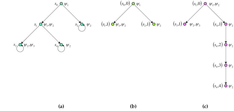
Figure 3: Examples of  $\mathbf{U}$ and $\mathbf{\widetilde{U}}$ unwinding.

Example 9.1

Consider the Kripke structure shown in Figure 3$(a)$. The $\mathbf{U}$ unwinding of $\mathbf{A}(\psi_{1}\mathbf{U}\psi_{2})$ from $s_{0}$ is shown in Figure 3$(b)$ and the $\mathbf{\widetilde{U}}$ unwinding of $\mathbf{A}(\psi_{3}\mathbf{\widetilde{U}}\psi_{2})$ from $s_{1}$ is depicted in Figure 3$(c)$. Note that in Figure 3$(c)$ $(s_{4},3)$ is an internal node whereas $(s_{4},4)$ is a leaf. $\blacktriangle$

Proposition 9.1

Let $\mathcal{K}=\langle W,R,V\rangle$ be a Kripke structure, let $\mathcal{K},s\models\mathbf{A}(\psi_{1}\mathbf{U}\psi_{2})$ and let $\mathcal{K}_{s}^{\mathbf{U}}$ be the $\mathbf{U}$ unwinding of $\mathcal{K}$ from $s$. Then the following hold:

1. If $(s^{\prime},n)$ is a leaf of $\mathcal{K}_{s}^{\mathbf{U}}$, then $\mathcal{K},s^{\prime}\models\psi_{2}$.

2. If $(s^{\prime},n)$ is an internal node of $\mathcal{K}_{s}^{\mathbf{U}}$, then $\mathcal{K},s^{\prime}\models\psi_{1}\wedge\neg\psi_{2}$. $\dashv$

Proposition 9.2

Let $\mathcal{K}=\langle W,R,V\rangle$ be a finite Kripke structure, let $\mathcal{K},s\models\mathbf{A}(\psi_{1}\mathbf{\widetilde{U}}\psi_{2})$ and let $\mathcal{K}_{s}^{\mathbf{\widetilde{U}}}$ be the $\mathbf{\widetilde{U}}$ unwinding of $\mathcal{K}$ from $s$. Then the following hold:

1. If $(s^{\prime},n)$ is a leaf of $\mathcal{K}_{s}^{\mathbf{\widetilde{U}}}$, then either

   1. $\mathcal{K},s^{\prime}\models\psi_{1}\wedge\psi_{2}$, or

   2. $n=|W|-1$, $\mathcal{K},s^{\prime}\models\neg\psi_{1}\wedge\psi_{2}$ and for every child $t$ of $s^{\prime}$, $\mathcal{K},t\models\psi_{2}$.

2. If $(s^{\prime},n)$ is an internal node of $\mathcal{K}_{s}^{\mathbf{\widetilde{U}}}$, then $n<|W|-1$ and also $\mathcal{K},s^{\prime}\models\neg\psi_{1}\wedge\psi_{2}$.

Proposition 9.3

Let $\mathcal{K}=\langle W,R,V\rangle$ be a finite Kripke structure and let $s_{0}$, …, $s_{i}$, …, $s_{j}$, …, $s_{n}$ be a finite path in $\mathcal{K}$ (or in the corresponding database $D$), where $n\geq|W|$. Then, there exists a state $s$ such that $s_{i}=s_{j}=s$.

9.2 Proof of Theorem 7.1

We are ready now to prove that (12) holds by induction on the structure of formula $\varphi$. To increase the readability of the proof, we use the subscripts in the goal predicates to denote the corresponding CTL formula. For instance, we write $G_{\mathbf{E}{\bigcirc}\psi}$ to denote that $G$ is the goal predicate of the program corresponding to $\mathbf{E}{\bigcirc}\psi$. We consider the two directions separately and begin by considering the $\Rightarrow$ direction.

Proof ($\Rightarrow$)

1. If $\varphi\equiv p$ or $\varphi\equiv\neg p$, where $p\in AP$, or $\varphi\equiv\top$, then the corresponding programs are those of Definition 7.2.(1). Trivially, then:

   • ${\mathcal{K}},s\models p\Rightarrow p\in V(s)\Rightarrow P(s)$ is a ground fact of $D\Rightarrow s\in G_{p}(D)$.

   • ${\mathcal{K}},s\models\neg p\Rightarrow p\not\in V(s)\Rightarrow P(s)$ is not a ground fact of $D\Rightarrow s\in G_{\neg p}(D)$.

   • ${\mathcal{K}},s\models\top\Rightarrow s\in W\Rightarrow$ (by the totality of $R$) there exists $t\in W$ such that $(s,t)\in S_{0}\cup S_{1}$ $\Rightarrow s\in W_{\Pi^{n}}(D)\Rightarrow s\in G_{\top}(D)$.

2. If $\varphi\equiv\psi_{1}\vee\psi_{2}$ or $\varphi\equiv\psi_{1}\wedge\psi_{2}$, then the corresponding programs are shown in Definition 7.2.(2). Again, the next hold:

   • ${\mathcal{K}},s\models\varphi\Rightarrow{\mathcal{K}},s\models\psi_{1}$ or ${\mathcal{K}},s\models\psi_{2}\Rightarrow$ (by the induction hypothesis) $s\in G_{\psi_{1}}(D)$ or $s\in G_{\psi_{2}}(D)\Rightarrow s\in G_{\psi_{1}}(D)\cup G_{\psi_{2}}(D)\Rightarrow s\in G_{\varphi}(D)$.

   • ${\mathcal{K}},s\models\varphi\Rightarrow{\mathcal{K}},s\models\psi_{1}$ and ${\mathcal{K}},s\models\psi_{2}\Rightarrow$ (by the induction hypothesis) $s\in G_{\psi_{1}}(D)$ and $s\in G_{\psi_{2}}(D)\Rightarrow s\in G_{\psi_{1}}(D)\cap G_{\psi_{2}}(D)\Rightarrow s\in G_{\varphi}(D)$.

3. If $\varphi\equiv\mathbf{E}{\bigcirc}\psi$, then the corresponding program is shown in Definition 7.2.(3).

   Let us assume that ${\mathcal{K}},\pi\models\varphi$ for some path $\pi=s_{0},s_{1},s_{2},\ldots$  with initial state $s_{0}$. We know that either $S_{0}(s_{0},s_{1})$ or $S_{1}(s_{0},s_{1})$ holds. Now ${\mathcal{K}},\pi\models\varphi$ for the path $\pi=s_{0},s_{1},s_{2}$, …$\Rightarrow$ ${\mathcal{K}},\pi^{1}\models\psi$ for the path $\pi^{1}=s_{1},s_{2},\ldots$ $\Rightarrow$ ${\mathcal{K}},s_{1}\models\psi$ $\Rightarrow$ (by the induction hypothesis) $s_{1}\in G_{\psi}(D)$. From $\Pi_{\varphi}$, by combining $G_{\psi}(s_{1})$ with one of $S_{0}(s_{0},s_{1})$ or $S_{1}(s_{0},s_{1})$, we immediately derive $G_{\varphi}(s_{0})$ and, thus, $s_{0}\in G_{\varphi}(D)$.

4. If $\varphi\equiv\mathbf{A}{\bigcirc}\psi$, then the corresponding program is shown in Definition 7.2.(3).

   Let’s assume now that ${\mathcal{K}},\pi\models\varphi$ for every path $\pi=s_{0},s_{1},s_{2},...$ with initial state $s_{0}$. It is convenient to distinguish two cases:
   (a)    $s_{0}$ has a left child $s_{1}^{L}$, but not a right child. In this case ${\mathcal{K}},\pi\models\varphi$  for every path $\pi=s_{0},s_{1},s_{2}$, … with initial state $s_{0}\Rightarrow{\mathcal{K}},\pi^{1,L}\models\psi$ for every path $\pi^{1,L}=s_{1}^{L},s_{2},\ldots$ with initial state $s_{1}^{L}$ $\Rightarrow$ ${\mathcal{K}},s_{1}^{L}\models\psi$ $\Rightarrow$ (by the induction hypothesis) $s_{1}^{L}\in G_{\psi}(D)$. Moreover, in this case $S_{0}(s_{0},s_{1}^{L})$, $\neg 2S(s_{0})$ are true and, therefore, evaluation of the second rule of $\Pi_{\varphi}$ gives $G_{\varphi}(s_{0})\longleftarrow S_{0}(s_{0},s_{1}^{L}),\neg 2S(s_{0}),G_{\psi}(s_{1}^{L})$ $\Rightarrow$ $s_{0}\in G_{\varphi}(D)$.
   (b)    $s_{0}$ has both a left child $s_{1}^{L}$ and a right child $s_{1}^{R}$. Then ${\mathcal{K}},\pi\models\varphi$ for every path $\pi=s_{0},s_{1},s_{2},\ldots$ with initial state $s_{0}$ $\Rightarrow$ ${\mathcal{K}},\pi^{1,L}\models\psi$  for every path $\pi^{1,L}=s_{1}^{L},s_{2}^{L},\ldots$ with initial state $s_{1}^{L}$ and ${\mathcal{K}},\pi^{1,R}\models\psi$  for every path $\pi^{1,R}=s_{1}^{R},s_{2}^{R},\ldots$ with initial state $s_{1}^{R}$ $\Rightarrow{\mathcal{K}},s_{1}^{L}\models\psi$ and ${\mathcal{K}},s_{1}^{R}\models\psi$ $\Rightarrow$ (by the induction hypothesis) $s_{1}^{L},s_{1}^{R}\in G_{\psi}(D)$. Moreover, in this case $S_{0}(s_{0},s_{1}^{L})$, $S_{1}(s_{0},s_{1}^{R})$ are true and, therefore, evaluation of the third rule of $\Pi_{\varphi}$ gives $G_{\varphi}(s_{0})$ $\longleftarrow$ $S_{0}(s_{0},s_{1}^{L})$, $S_{1}(s_{0},s_{1}^{R})$, $G_{\psi}(s_{1}^{L})$, $G_{\psi}(s_{1}^{R})$ $\Rightarrow$ $s_{0}\in G_{\varphi}(D)$.

5. If $\varphi\equiv\mathbf{E}(\psi_{1}\mathbf{U}\psi_{2})$, then the corresponding program is this of Definition 7.2.(3).

   Suppose that ${\mathcal{K}},\pi\models\varphi$ where the path $\pi$ is $s_{0},s_{1},$ $s_{2},\ldots$  . We have to examine two cases:
   (a)    ${\mathcal{K}},\pi\models\psi_{2}$ for the path $\pi=s_{0},s_{1},s_{2},\ldots$ $\Rightarrow$ ${\mathcal{K}},s_{0}\models\psi_{2}$ $\Rightarrow$ (by the induction hypothesis) $s_{0}\in G_{\psi_{2}}(D)$ $\Rightarrow$ $G_{\varphi}(s_{0})$ (from the first rule $G_{\varphi}(x)\longleftarrow G_{\psi_{2}}(x)$ of $\Pi_{\varphi}$) $\Rightarrow$ $s_{0}\in G_{\varphi}(D)$.
   (b)    ${\mathcal{K}},\pi^{i}\models\psi_{2}$ for the path $\pi^{i}=s_{i},s_{i+1},s_{i+2}$, … and ${\mathcal{K}},\pi^{j}\models\psi_{1}$ for $\pi^{j}=s_{j},s_{j+1},s_{j+2},\ldots$ $(0\leq j\leq i-1)$ $\Rightarrow$ ${\mathcal{K}},s_{i}\models\psi_{2}$ and ${\mathcal{K}},s_{j}\models\psi_{1}$ $(0\leq j\leq i-1)$ $\Rightarrow$ $s_{i}\in G_{\psi_{2}}(D)$ and $s_{j}\in G_{\psi_{1}}(D_{\mathcal{K}})$ $(0\leq j\leq i-1)$ (by the induction hypothesis). We know that for every $r$, $0\leq r<i$, at least one of $S_{0}(s_{r},s_{r+1})$ or $S_{1}(s_{r},s_{r+1})$ holds. From the first rule $G_{\varphi}(x)\longleftarrow G_{\psi_{2}}(x)$ of $\Pi_{\varphi}$ we derive that $G_{\varphi}(s_{i})$. Successive applications of the second ($G_{\varphi}(s_{r})$ $\longleftarrow$ $G_{\psi_{1}}(s_{r})$, $S_{0}(s_{r},s_{r+1})$, $G_{\varphi}(s_{r+1})$) and third rule ($G_{\varphi}(s_{r})$ $\longleftarrow$ $G_{\psi_{1}}(s_{r})$, $S_{1}(s_{r},s_{r+1})$, $G_{\varphi}(s_{r+1})$) of $\Pi_{\varphi}$ for every $r$, $0\leq r<i$, yield $G_{\varphi}(s_{i-1})$, $G_{\varphi}(s_{i-2})$, …, $G_{\varphi}(s_{1})$, $G_{\varphi}(s_{0})$. Thus, $s_{0}\in G_{\varphi}(D)$.

6. If $\varphi\equiv\mathbf{A}(\psi_{1}\mathbf{U}\psi_{2})$, then the corresponding program is this of Definition 7.2.(3).

   Let us assume now that ${\mathcal{K}},\pi\models\varphi$ for every path $\pi=s_{0},s_{1},s_{2},\ldots$  with initial state $s_{0}$. Consider the $\mathbf{U}$ unwinding $\mathcal{K}_{s_{0}}^{\mathbf{U}}$ of ${\mathcal{K}}$ from $s_{0}$ and let $(t_{0},r)$ be any node of $\mathcal{K}_{s_{0}}^{\mathbf{U}}$; we shall prove that $t_{0}\in G_{\varphi}(D)$. This property of $\mathcal{K}_{s_{0}}^{\mathbf{U}}$ indeed implies the required result because $(s_{0},0)$ is a node (specifically the root) of $\mathcal{K}_{s_{0}}^{\mathbf{U}}$ and, thus, $s_{0}\in G_{\varphi}(D)$. To prove it, let $L_{t_{0}}=(t_{0},r),(t_{1},r+1),\ldots,(t_{n},r+n)$ be the longest path from $(t_{0},r)$ to a leaf $(t_{n},r+n)$ of $\mathcal{K}_{s_{0}}^{\mathbf{U}}$. We use induction on the length $n$ of the path $L_{t_{0}}$.
   (a)    If $n=0$, then node $(t_{0},r)$ itself is a leaf. From Proposition 9.1 we know that ${\mathcal{K}},t_{0}\models\psi_{2}$ and by the induction hypothesis (pertaining to formula $\psi_{2}$) we get that $t_{0}\in G_{\psi_{2}}(D)$. Then, from rule $G_{\varphi}(x)\longleftarrow G_{\psi_{2}}(x)$ of $\Pi_{\varphi}$, we derive that $G_{\varphi}(t_{0})$.
   (b)    We show now that the claim holds for paths of length $n+1$, assuming that it holds for paths of length less than or equal to $n$. In this case node $(t_{0},r)$ is an internal node of $\mathcal{K}_{s_{0}}^{\mathbf{U}}$. From Proposition 9.2 we know that ${\mathcal{K}},t_{0}\models\psi_{1}$ and by the induction hypothesis (pertaining to formula $\psi_{1}$) we get that $t_{0}\in G_{\psi_{1}}(D)$. We focus on the case where node $(t_{0},r)$ has exactly two successors $(t^{L}_{1},r+1)$ and $(t^{R}_{1},r+1)$ in $\mathcal{K}_{s_{0}}^{\mathbf{U}}$ (the case where $(t_{0},r)$ has only one successor is easier). Since $L_{t_{0}}$ has length $n+1$, then both $L_{t^{L}_{1}}$ and $L_{t^{R}_{1}}$ have length at most $n$. Hence, by the induction hypothesis with respect to the length of the paths $L_{t^{L}_{1}}$ and $L_{t^{R}_{1}}$, we get that $t_{1}^{L}\in G_{\varphi}(D)$ and $t_{1}^{R}\in G_{\varphi}(D)$. So $G_{\psi_{1}}(t_{0})$, $S_{0}(t_{0},t_{1}^{L})$, $S_{1}(t_{0},t_{1}^{R})$, $G_{\varphi}(t_{1}^{L})$ and $G_{\varphi}(t_{1}^{R})$ are true and, therefore, the evaluation of the third rule of $\Pi_{\varphi}$ gives that $G_{\varphi}(t_{0})$ $\longleftarrow$ $G_{\psi_{1}}(t_{0})$, $S_{0}(t_{0},t_{1}^{L})$, $S_{1}(t_{0},t_{1}^{R})$, $G_{\varphi}(t_{1}^{L})$, $G_{\varphi}(t_{1}^{R})$. Thus, $t_{0}\in G_{\varphi}(D)$.

7. If $\varphi\equiv\mathbf{E}(\psi_{1}\mathbf{\widetilde{U}}\psi_{2})$, then the corresponding program is shown in Definition 7.2.(3).

   Suppose that ${\mathcal{K}},\pi\models\varphi$ where the path $\pi$ is $s_{0},s_{1}$, $s_{2},\ldots$  . We must consider two cases:
   (a)    ${\mathcal{K}},\pi^{i}\models\psi_{1}\wedge\psi_{2}$ for the path $\pi^{i}=s_{i},s_{i+1}$, $s_{i+2}$, … and ${\mathcal{K}},\pi^{j}\models\psi_{2}$ for $\pi^{j}=s_{j},s_{j+1}$, $s_{j+2}$, … $(0\leq j\leq i-1)$ $\Rightarrow$ ${\mathcal{K}},s_{i}\models\psi_{1}\wedge\psi_{2}$ and ${\mathcal{K}},s_{j}\models\psi_{2}$ $(0\leq j\leq i-1)$ $\Rightarrow$ $s_{i}\in G_{\psi_{1}}(D)$ and $s_{j}\in G_{\psi_{2}}(D)$ $(0\leq j\leq i)$ (by the induction hypothesis). We know that for every $r$, $0\leq r<i$, at least one of $S_{0}(s_{r},s_{r+1})$ or $S_{1}(s_{r},s_{r+1})$ holds. From rule $G_{\varphi}(x)\longleftarrow G_{\psi_{1}}(x),G_{\psi_{2}}(x)$ of $\Pi_{\varphi}$ we derive that $G_{\varphi}(s_{i})$. Successive applications of the other two rules of the program (i.e., $G_{\varphi}(s_{r})$ $\longleftarrow$ $G_{\psi_{2}}(s_{r})$, $S_{0}(s_{r},s_{r+1})$, $G_{\varphi}(s_{r+1})$ and $G_{\varphi}(s_{r})$ $\longleftarrow$ $G_{\psi_{2}}(s_{r})$, $S_{1}(s_{r},s_{r+1})$, $G_{\varphi}(s_{r+1})$) for every $r$, $0\leq r<i$, yield $G_{\varphi}(s_{i-1})$, $G_{\varphi}(s_{i-2})$, …, $G_{\varphi}(s_{1})$, $G_{\varphi}(s_{0})$. Thus, $s_{0}\in G_{\varphi}(D)$.
   (b)    ${\mathcal{K}},\pi^{i}\models\psi_{2}$ for the path $\pi^{i}=s_{i},s_{i+1},s_{i+2}$, …, for every $i\geq 0$. This implies that ${\mathcal{K}},s_{i}\models\psi_{2}$, for every $i\geq 0$, and (by the induction hypothesis) that $s_{i}\in G_{\psi_{2}}(D)$, for every $i\geq 0$. Let $s_{0},s_{1},s_{2},\ldots,s_{n}$ be an initial segment of $\pi$, where $n=|W|$. From Proposition 9.3 we know that in the aforementioned sequence there exists a state $s$ such that $s=s_{k}=s_{l}$, $0\leq k<l\leq n$. Then $(s_{k},s_{k})\in B_{\psi_{2}}(D)$. We know that for every $r$, $0\leq r<k$, at least one of $S_{0}(s_{r},s_{r+1})$ or $S_{1}(s_{r},s_{r+1})$ holds. From rule $G_{\varphi}(x)\longleftarrow B_{\psi_{2}}(x,x)$ we derive that $G_{\varphi}(s_{k})$. Successive applications of the fourth ($G_{\varphi}(s_{r})$ $\longleftarrow$ $G_{\psi_{2}}(s_{r})$, $S_{0}(s_{r},s_{r+1})$, $G_{\varphi}(s_{r+1})$) or the fifth ($G_{\varphi}(s_{r})$ $\longleftarrow$ $G_{\psi_{2}}(s_{r})$, $S_{1}(s_{r},s_{r+1})$, $G_{\varphi}(s_{r+1})$) rule of $\Pi_{\varphi}$ for every $r$, $0\leq r<k$, yield $G_{\varphi}(s_{k-1})$, $G_{\varphi}(s_{k-2})$, …, $G_{\varphi}(s_{1})$, $G_{\varphi}(s_{0})$. Accordingly, $s_{0}\in G_{\varphi}(D)$.

8. If $\varphi\equiv\mathbf{A}(\psi_{1}\mathbf{\widetilde{U}}\psi_{2})$, then the corresponding program is shown in Definition 7.2.(3).

   Let us assume now that ${\mathcal{K}},\pi\models\varphi$ for every path $\pi=s_{0},s_{1},s_{2},\ldots$ with initial state $s_{0}$. Consider the $\mathbf{\widetilde{U}}$ unwinding $\mathcal{K}_{s_{0}}^{\mathbf{\widetilde{U}}}$ of ${\mathcal{K}}$ from $s_{0}$ and let $(t_{0},r)$ be any node of $\mathcal{K}_{s_{0}}^{\mathbf{\widetilde{U}}}$. We shall prove that either $G_{\varphi}(t_{0})$ or $C_{\psi_{2}}(t_{0},|W|-r)$ holds. This property of the nodes of $\mathcal{K}_{s_{0}}^{\mathbf{\widetilde{U}}}$ ensures that for the root $(s_{0},0)$ it must be the case that $s_{0}\in G_{\varphi}(D)$ (recall the universal program in Section 5). To prove this property, let $L_{t_{0}}=(t_{0},r)$, $(t_{1},r+1)$, …, $(t_{n},r+n)$ be the longest path from $(t_{0},r)$ to a leaf $(t_{n},r+n)$ of $\mathcal{K}_{s_{0}}^{\mathbf{\widetilde{U}}}$. We are going to use induction on the length $n$ of the path $L_{t_{0}}$.
   (a)    If $n=0$, then node $(t_{0},r)$ itself is a leaf. We may assume that node $t_{0}$ has exactly two successors $t^{L}_{1}$ and $t^{R}_{1}$ in $D$ because the case where $t_{0}$ has only one successor can be tackled in the same way. From Proposition 9.2 we know that there are two cases regarding $t_{0}$: (1) ${\mathcal{K}},t_{0}\models\psi_{1}\wedge\psi_{2}$; in this case the induction hypothesis (with respect to $\psi_{1}$ and $\psi_{2}$) gives that $t_{0}\in G_{\psi_{1}}(D)$ and $t_{0}\in G_{\psi_{2}}(D)$ and from the first rule of $\Pi_{\varphi}$ we derive that $G_{\varphi}(t_{0})$. (2) $r=|W|-1$, ${\mathcal{K}},t_{0}\models\neg\psi_{1}\wedge\psi_{2}$ and ${\mathcal{K}},t^{L}_{1}\models\psi_{2}$ and ${\mathcal{K}},t^{R}_{1}\models\psi_{2}$. The induction hypothesis with respect to $\psi_{2}$ gives that $t_{0}\in G_{\psi_{2}}(D)$, $t^{L}_{1}\in G_{\psi_{2}}(D)$ and $t^{R}_{1}\in G_{\psi_{2}}(D)$. Using rule $C_{\psi_{2}}(t_{0},1)\longleftarrow G_{\psi_{2}}(t_{0})$, $S_{0}(t_{0},t^{L}_{1})$, $S_{1}(t_{0},t^{R}_{1})$, $G_{\psi_{2}}(t^{L}_{1})$, $G_{\psi_{2}}(t^{R}_{1})$ of $\Pi_{\varphi}^{\mathbf{A}}$ we conclude that $C_{\psi_{2}}(t_{0},1)$ holds.
   (b)    We prove now that the claim holds for paths of length $n+1$, assuming that it holds for paths of length less than or equal to $n$. In this case node $(t_{0},r)$ is an internal node of $\mathcal{T}_{s_{0}}^{\mathbf{\widetilde{U}}}$. From Proposition 9.2 we know that $r<|W|-1$ and ${\mathcal{K}},t_{0}\models\neg\psi_{1}\wedge\psi_{2}$ and by the induction hypothesis (pertaining to $\psi_{2}$) we get that $t_{0}\in G_{\psi_{2}}(D)$. We examine the case where node $(t_{0},r)$ has exactly two successors $(t^{L}_{1},r+1)$ and $(t^{R}_{1},r+1)$ in $\mathcal{K}_{s_{0}}^{\mathbf{\widetilde{U}}}$, where $r+1<|W|$. In this case $S_{0}(t_{0},t_{1}^{L})$, $S_{1}(t_{0},t_{1}^{R})$ are true. Since $L_{t_{0}}$ has length $n+1$, then both $L_{t^{L}_{1}}$ and $L_{t^{R}_{1}}$ have length at most $n$. Hence, by the induction hypothesis (regarding the path length), we get that $G_{\varphi}(t_{1}^{L})$ or $C_{\psi_{2}}(t_{1}^{L},|W|-r-1)$ and $G_{\varphi}(t_{1}^{R})$ or $C_{\psi_{2}}(t_{1}^{R},|W|-r-1)$. If $G_{\varphi}(t_{1}^{L})$ and $G_{\varphi}(t_{1}^{R})$ are true, then the third rule of $\Pi_{\varphi}$ ($G_{\varphi}(x)$ $\longleftarrow$ $G_{\psi_{2}}(x)$, $S_{0}(x,y)$, $S_{1}(x,z)$, $G_{\varphi}(y)$, $G_{\varphi}(z)$) implies that $G_{\varphi}(t_{0})$ also holds. If $C_{\psi_{2}}(t_{1}^{L},|W|-r-1)$ and $C_{\psi_{2}}(t_{1}^{R},|W|-r-1)$ are true, then using the seventh rule of $\Pi_{\varphi}(C_{\psi_{2}}(x,n)$ $\longleftarrow$ $G_{\psi_{2}}(x)$, $S_{0}(x,y)$, $S_{1}(x,z)$, $C_{\psi_{2}}(y,n-1)$, $C_{\psi_{2}}(z,n-1)$, $n\leq|W|$) we conclude that $C_{\psi_{2}}(t_{0},|W|-r)$ also holds. In the remaining two cases the eighth and ninth rule imply that $C_{\psi_{2}}(t_{0},|W|-r)$.

   We have proved that for the node $(s_{0},0)$ one of $G_{\varphi}(s_{0})$ or $C_{\psi_{2}}(s_{0},|W|)$ holds. If we assume that $C_{\psi_{2}}(s_{0},|W|)$ holds, then the fifth rule of $\Pi_{\varphi}$ implies $G_{\varphi}(s_{0})$. Hence, in any case, $s_{0}\in G_{\varphi}(D)$. $\dashv$

We complete now the proof of (12) by examining the opposite direction.

Proof ($\Leftarrow$)

1. If $\varphi\equiv p$ or $\varphi\equiv\neg p$, where $p\in AP$, or $\varphi\equiv\top$, then the corresponding programs are those of Definition 7.2.(1). Trivially, then:

   • $s\in G_{p}(D)\Rightarrow P(s)$ is a ground fact of $D\Rightarrow p\in V(s)\Rightarrow{\mathcal{K}},s\models p$.

   • $s\in G_{\neg p}(D)\Rightarrow P(s)$ is not a ground fact of $D\Rightarrow p\not\in V(s)\Rightarrow{\mathcal{K}},s\models\neg p$.

   • $s\in G_{\top}(D)\Rightarrow s\in W_{\Pi^{n}}(D)\Rightarrow s$ appears in one of $S_{0},S_{1},P_{0},\ldots,P_{n}\Rightarrow s\in W\Rightarrow{\mathcal{K}},s\models\top$.

2. If $\varphi\equiv\psi_{1}\vee\psi_{2}$ or $\varphi\equiv\psi_{1}\wedge\psi_{2}$, then the corresponding programs are shown in Definition 7.2.(2). Again, the following hold:

   • $s\in G_{\varphi}(D)\Rightarrow s\in G_{\psi_{1}}(D)\cup G_{\psi_{2}}(D_{\mathcal{K}})\Rightarrow s\in G_{\psi_{1}}(D)$ or $s\in G_{\psi_{2}}(D)\Rightarrow$ (by the induction hypothesis) ${\mathcal{K}},s\models\psi_{1}$ or ${\mathcal{K}},s\models\psi_{2}\Rightarrow{\mathcal{K}},s\models\varphi$.

   • $s\in G_{\varphi}(D)\Rightarrow s\in G_{\psi_{1}}(D)\cap G_{\psi_{2}}(D_{\mathcal{K}})\Rightarrow s\in G_{\psi_{1}}(D)$ and $s\in G_{\psi_{2}}(D)\Rightarrow$ (by the induction hypothesis) ${\mathcal{K}},s\models\psi_{1}$ and ${\mathcal{K}},s\models\psi_{2}\Rightarrow{\mathcal{K}},s\models\varphi$.

3. If $\varphi\equiv\mathbf{E}{\bigcirc}\psi$, then the corresponding program is shown in Definition 7.2.(3).

   Let us assume that $s_{0}\in G_{\varphi}(D)$. From the rules of the program $\Pi_{\varphi}$ we see that there exists a $s_{1}$ such that $G_{\psi}(s_{1})$ and also one of $S_{0}(s_{0},s_{1})$ or $S_{1}(s_{0},s_{1})$ holds. By the induction hypothesis we get ${\mathcal{K}},s_{1}\models\psi$. Let $\pi=s_{0},s_{1},s_{2},\ldots$ be any path with initial state $s_{0}$ and second state $s_{1}$. Clearly, then ${\mathcal{K}},\pi^{1}\models\psi$ for the path $\pi^{1}=s_{1},s_{2},\ldots$ and ${\mathcal{K}},\pi\models\varphi$ for the path $\pi=s_{0},s_{1},s_{2},\ldots$.

4. If $\varphi\equiv\mathbf{A}{\bigcirc}\psi$, then the corresponding program is shown in Definition 7.2.(3).

   Suppose now that $s_{0}\in G_{\varphi}(D)$. It is convenient to distinguish two cases:
   (a)    $s_{0}$ has a left successor $s_{1}^{L}$ but not a right successor in $D$; in this case $S_{0}(s_{0},s_{1}^{L})$ and $\neg 2S(s_{0})$ are true. From the second rule of $\Pi_{\varphi}$ we see that $G_{\psi}(s_{1}^{L})$ holds. By the induction hypothesis we get ${\mathcal{K}},s_{1}^{L}\models\psi$. Let $\pi=s_{0},s_{1},s_{2},\ldots$ be an arbitrary path with initial state $s_{0}$. The fact that $s_{0}$ has a left successor $s_{1}^{L}$ but not a right successor implies that $s_{1}^{L}$ is the second state of every such path. Suppose that there exists a path $\pi=s_{0},s_{1}^{L},s_{2},\ldots$ with initial state $s_{0}$ such that ${\mathcal{K}},\pi\not\models\varphi$. Trivially then ${\mathcal{K}},\pi^{1}\not\models\psi$, where $\pi^{1}=s_{1}^{L},s_{2},\ldots$, which in turn implies that ${\mathcal{K}},s_{1}^{L}\not\models\psi$, which is false.
   (b)    $s_{0}$ has both a left successor $s_{1}^{L}$ and a right successor $s_{1}^{R}$ in $D$; in this case $S_{0}(s_{0},s_{1}^{L})$ and $S_{1}(s_{0},s_{1}^{R})$ are true. From the third rule of $\Pi_{\varphi}$ we see that $G_{\psi}(s_{1}^{L})$ and $G_{\psi}(s_{1}^{R})$ hold. By the induction hypothesis we get ${\mathcal{K}},s_{1}^{L}\models\psi$ and ${\mathcal{K}},s_{1}^{R}\models\psi$. Let $\pi=s_{0},s_{1},s_{2},\ldots$ be an arbitrary path with initial state $s_{0}$. The fact that $s_{0}$ has both a left successor $s_{1}^{L}$ and a right successor $s_{1}^{R}$ implies that either $s_{1}^{L}$ or $s_{1}^{R}$ is the second state of every such path. Suppose that there exists a path $\pi=s_{0},s_{1},s_{2},\ldots$ with initial state $s_{0}$ such that ${\mathcal{K}},\pi\not\models\varphi$. If that were the case, then ${\mathcal{K}},\pi^{1}\not\models\psi$, where $\pi^{1}=s_{1},s_{2},\ldots$  . But $s_{1}=s_{1}^{L}$ or $s_{1}=s_{1}^{R}$, which means that ${\mathcal{K}},s_{1}^{L}\not\models\psi$ or ${\mathcal{K}},s_{1}^{R}\not\models\psi$, either of which contradicts the induction hypothesis.

5. If $\varphi\equiv\mathbf{E}(\psi_{1}\mathbf{U}\psi_{2})$, then the corresponding program is this of Definition 7.2.(3).

   Suppose that $s_{0}\in G_{\varphi}(D)$. From the rules of the program $\Pi_{\varphi}$ we see that there exists a $s_{i}$ (possibly $s_{i}=s_{0}$) such that $G_{\psi_{2}}(s_{i})$ holds. Further, there exists a sequence of states $s_{0},s_{1},\ldots,s_{i}$ such that for every $r$ ($0\leq r<i$) $G_{\psi_{1}}(s_{r})$ and at least one of $S_{0}(s_{r},s_{r+1})$ or $S_{1}(s_{r},s_{r+1})$ is true. By the induction hypothesis we get ${\mathcal{K}},s_{i}\models\psi_{2}$ and ${\mathcal{K}},s_{j}\models\psi_{1}$ $(0\leq j\leq i-1)$. Let $\pi=s_{0},s_{1},s_{2},\ldots,s_{i},\ldots$ be any path with initial segment $s_{0},s_{1},\ldots,s_{i}$; then ${\mathcal{K}},\pi^{i}\models\psi_{2}$ and ${\mathcal{K}},\pi^{j}\models\psi_{1}$ $(0\leq j\leq i-1)$, i.e., ${\mathcal{K}},\pi\models\varphi$.

6. If $\varphi\equiv\mathbf{A}(\psi_{1}\mathbf{U}\psi_{2})$ then the corresponding program is this of Definition 7.2.(3).

   Let us assume now that $s_{0}\in G_{\varphi}(D)$. Let us define $G_{\varphi}(D,n)$ to be the set of ground facts for $G_{\varphi}$ that have been computed in the first $n$ rounds of the evaluation of program $\Pi_{\varphi}$. For more details in the bottom-up evaluation of Datalog programs see [Ull88]. We shall prove that for every $t\in G_{\varphi}(D,n)$, ${\mathcal{K}},\pi\models\varphi$ for every path $\pi=t_{0},t_{1},t_{2},\ldots$  with initial state $t_{0}=t$. We use induction on the number of rounds $n$.
   (a)    If $n=1$, then $t$ appears in $G_{\varphi}(D)$ due to the first rule of $\Pi_{\varphi}$, i.e., $t\in G_{\psi_{2}}(D)$. By the induction hypothesis with respect to $\psi_{2}$ we get that ${\mathcal{K}},t\models\psi_{2}$, which trivially implies that ${\mathcal{K}},\pi\models\varphi$ for every path $\pi=t_{0},t_{1},t_{2},\ldots$  with initial state $t_{0}=t$.
   (b)    We show now that the claim holds for $n+1$, assuming that it holds for $n$. We examine only the case where node $t$ has exactly two successors $t^{L}$ and $t^{R}$, since the case where $t$ has only one successor is identical. Without loss of generality we may assume that $t$ first appeared in $G_{\varphi}(D,n+1)$ during round $n+1$. This must have happened due to the third rule of $\Pi_{\varphi}$: $G_{\varphi}(x)$ $\longleftarrow$ $G_{\psi_{1}}(x)$, $S_{0}(x,y)$, $S_{1}(x,z)$, $G_{\varphi}(y)$, $G_{\varphi}(z)$. This implies that $t\in G_{\psi_{1}}(D)$ and both $t^{L}$ and $t^{R}$ belong to $G_{\varphi}(D,n)$. Hence, by invoking the induction hypothesis with respect to $\psi_{1}$ we get that ${\mathcal{K}},t\models\psi_{1}$, and by the induction hypothesis with respect to the number of rounds we get that ${\mathcal{K}},\pi^{1,L}\models\varphi$ for every path $\pi^{1,L}=t_{1}^{L},t_{2}^{L},\ldots$  with initial state $t_{1}^{L}=t^{L}$ and ${\mathcal{K}},\pi^{1,R}\models\varphi$ for every path $\pi^{1,R}=t_{1}^{R},t_{2}^{R},\ldots$  with initial state $t_{1}^{R}=t^{R}$. By combining all these, we conclude that ${\mathcal{K}},\pi\models\varphi$ for every path $\pi=t_{0},t_{1},t_{2},\ldots$  with initial state $t_{0}=t$.

   Note that the bottom-up evaluation of Datalog programs guarantees that there exists $n\in\mathbb{N}$ such that $G_{\varphi}(D,n)=G_{\varphi}(D,r)$ for every $r>n$, i.e., $G_{\varphi}(D)=G_{\varphi}(D,n)$.

7. If $\varphi\equiv\mathbf{E}(\psi_{1}\mathbf{\widetilde{U}}\psi_{2})$, then the corresponding program is shown in Definition 7.2.(3).

   Let us assume that $s_{0}\in G_{\varphi}(D)$. Let us define $G_{\varphi}(D,n)$ to be the set of ground facts for $G_{\varphi}$ that have been computed in the first $n$ rounds of the evaluation of program $\Pi_{\varphi}$. We shall prove that for every $t\in G_{\varphi}(D,n)$, there exists a path $\pi=t_{0},t_{1},t_{2},\ldots$  with initial state $t_{0}=t$, such that ${\mathcal{K}},\pi\models\varphi$. We use induction on the number of rounds $n$.
   (a)    If $n=1$, then $t$ appears in $G_{\varphi}(D)$ due to either the first rule, i.e., $t\in G_{\psi_{1}}(D)\cap G_{\psi_{2}}(D)$, or to the third rule, i.e., $(t,t)\in B_{\psi_{2}}(D)$. In the first case, the induction hypothesis pertaining to $\psi_{1}$ and $\psi_{2}$, implies that ${\mathcal{K}},t\models\psi_{1}\wedge\psi_{2}$, which immediately implies that ${\mathcal{K}},\pi\models\varphi$ for any path $\pi=t_{0},t_{1},t_{2},\ldots$ with initial state $t_{0}=t$. In the second case, there is a finite sequence $t_{0},t_{1},\ldots,t_{k}$ of states, such that $t_{0}=t_{k}=t$ and $t_{j}\in G_{\psi_{2}}(D)$,  $0\leq j\leq k$. Thus, by the induction hypothesis, ${\mathcal{K}},t_{j}\models\psi_{2}$,  $0\leq j\leq k$. Consider the path $\pi=(t_{0},t_{1},\ldots,t_{k})^{\omega}$; for this path we have ${\mathcal{K}},\pi\models\varphi$.
   (b)    We show now that the claim holds for $n+1$, assuming that it holds for $n$. We focus on the case where node $t$ has exactly two successors $t^{L}$ and $t^{R}$ (the case where $t$ has only one successor is similar). We may further assume that $t$ first appeared in $G_{\varphi}(D,n+1)$ during round $n+1$. This can only have occurred because of the fourth or fifth rule of $\Pi_{\varphi}$. Then $t\in G_{\psi_{2}}(D)$ and at least one of $t^{L}$ and $t^{R}$ belongs to $G_{\varphi}(D,n)$. Without loss of generality, we assume that $t^{L}\in G_{\varphi}(D,n)$. By the induction hypothesis, we know that ${\mathcal{K}},t\models\psi_{2}$ and that there exists a path $\pi^{1}=t_{1},t_{2},\ldots$  with initial state $t_{1}=t^{L}$, such that ${\mathcal{K}},\pi^{1}\models\varphi$. Immediately then we conclude that ${\mathcal{K}},\pi\models\varphi$, for the path $\pi=t_{0},t_{1},t_{2},\ldots$  with $t_{0}=t$.

   Note that the bottom-up evaluation of Datalog programs guarantees that there exists $n\in\mathbb{N}$ such that $G_{\varphi}(D,n)=G_{\varphi}(D,r)$ for every $r>n$, i.e., $G_{\varphi}(D)=G_{\varphi}(D,n)$.

8. If $\varphi\equiv\mathbf{A}(\psi_{1}\mathbf{\widetilde{U}}\psi_{2})$, where $\psi_{1}$ and $\psi_{2}$ are state formulae, then the corresponding program is shown in Definition 7.2.(3).

   Let us suppose now that $s_{0}\in G_{\varphi}(D)$. Let us define $G_{\varphi}(D,k)$ to be the set of ground facts for $G_{\varphi}$ that have been computed after $k$ rounds of the evaluation of program $\Pi_{\varphi}$. We shall prove with simultaneous induction on the number of rounds $k$ two things:
   (1)    Let $s\in G_{\varphi}(D,k)$ and let $\pi=s_{0},s_{1},\ldots$ be an arbitrary path with initial state $s_{0}=s$; then ${\mathcal{K}},\pi\models\psi_{1}\mathbf{\widetilde{U}}\psi_{2}$
   (2)    Let t be a state such that $C_{\psi_{2}}(t,k)$ holds (here of course $k\leq|W|$) and let $\varrho=t_{0},t_{1},$ …,$t_{k},\ldots$ be an arbitrary path with initial state $t_{0}=t$; then either ${\mathcal{K}},\varrho\models\psi_{1}\mathbf{\widetilde{U}}\psi_{2}$ or ${\mathcal{K}},t_{j}\models\psi_{2}$, for $0\leq j\leq k$.
   (a)    If $k=1$, then $s$ appears in $G_{\varphi}(D)$ due to the first rule of $\Pi_{\varphi}$, i.e., $s\in G_{\psi_{1}}(D)\cap G_{\psi_{2}}(D)$. Hence, ${\mathcal{K}},\pi\models\psi_{1}\mathbf{\widetilde{U}}\psi_{2}$, where $\pi=s_{0},s_{1},\ldots$ is any path with initial state $s_{0}=s$. We assume of course that $|W|>1$ because the case where $|W|=1$, that is the database contains only one element, is trivial. Similarly, for any state t, if $C_{\psi_{2}}(t,1)$ holds then $C_{\psi_{2}}(t,1)$ can only be derived by the tenth or eleventh rule of $\Pi_{\varphi}$. In any case, these rules imply that for every path $\pi=t_{0},t_{1},\ldots$ with initial state $t_{0}=t$ we have that ${\mathcal{K}},t_{0}\models\psi_{2}$ and ${\mathcal{K}},t_{1}\models\psi_{2}$.
   (b)    We show now that the claim holds for $k+1$, assuming that it holds for $k$. We consider the case where states $s$ and $t$ have exactly two successors $s^{L},s^{R}$ and $t^{L},t^{R}$, respectively.
   (i)    Initially, we shall consider the case where $k+1\leq|W|$.

   We may assume that $s$  first appeared in $G_{\varphi}(D,k+1)$ during round $k+1$. It is important to stress that in this case, $s$ cannot arise from an application of the fifth rule of $\Pi_{\varphi}$ because the first time this may happen is at round $|W|+1$. This implies that $s$ must have appeared because of the fourth rule $G_{\varphi}(x)$ $\longleftarrow$ $G_{\psi_{2}}(x)$, $S_{0}(x,y)$, $S_{1}(x,z)$, $G_{\varphi}(y)$, $G_{\varphi}(z)$. Hence, $s\in G_{\psi_{2}}(D)$ and both of $s^{L}$ and $s^{R}$ belong to $G_{\varphi}(D,k)$. Then, by the induction hypothesis, we get that ${\mathcal{K}},s\models\psi_{2}$, ${\mathcal{K}},\pi^{1,L}\models\varphi$ for every path $\pi^{1,L}=s_{1}^{L},s_{2}^{L},\ldots$  with initial state $s_{1}^{L}=s^{L}$ and ${\mathcal{K}},\pi^{1,R}\models\varphi$ for every path $\pi^{1,R}=s_{1}^{R},s_{2}^{R},\ldots$  with initial state $s_{1}^{R}=t^{R}$. Therefore, ${\mathcal{K}},\pi\models\varphi$  for every path $\pi=s_{0},s_{1},s_{2},\ldots$  with initial state $s_{0}=s$.

   Moreover, if $C_{\psi_{2}}(t,k+1)$ holds, then $G_{\psi_{2}}(t)$ holds and one of the next must also hold:
   - $C_{\psi_{2}}(t^{L},k)$ and $C_{\psi_{2}}(t^{R},k)$,
   - $G_{\varphi}(t^{L})$ and $C_{\psi_{2}}(t^{R},k)$, or
   - $C_{\psi_{2}}(t^{L},k)$ and $G_{\varphi}(t^{R})$.

   Thus, by the induction hypothesis, we know that:
   - ${\mathcal{K}},t\models\psi_{2}$, and
   - for every path $\varrho^{1,L}=t_{1}^{L},t_{2}^{L},\ldots,t_{k+1}^{L},\ldots$  with initial state $t_{1}^{L}=t^{L}$ either ${\mathcal{K}},\varrho^{1,L}\models\varphi$ or ${\mathcal{K}},t_{j}^{L}\models\psi_{2}$ ($1\leq j\leq k+1$), and
   - for every path $\varrho^{1,R}=t_{1}^{R},t_{2}^{R},\ldots,t_{k+1}^{R},\ldots$  with initial state $t_{1}^{R}=t^{R}$ either ${\mathcal{K}},\varrho^{1,R}\models\varphi$ or ${\mathcal{K}},t_{j}^{R}\models\psi_{2}$ ($1\leq j\leq k+1$).

   Taking all these into account, we conclude that for every path $\varrho$ $=t_{0}$,$t_{1}$, $t_{2},$ $\ldots$,$t_{k+1}$, $\ldots$  with initial state $t_{0}=t$ either ${\mathcal{K}},\varrho\models\varphi$ or ${\mathcal{K}},t_{j}\models\psi_{2}$ ($0\leq j\leq k+1$).
   (ii)    Finally, we examine the case where $k+1>|W|$.

   In this case, $s$ may belong to $G_{\varphi}(D,k+1)$ either due to the fourth rule ($G_{\varphi}(x)$ $\longleftarrow$ $G_{\psi_{2}}(x)$, $S_{0}(x,y)$, $S_{1}(x,z)$, $G_{\varphi}(y)$, $G_{\varphi}(z)$) or due to the fifth rule ($G_{\varphi}(x)\longleftarrow C_{\psi_{2}}(x,\mathbf{c}_{max})$). If it is due to the fourth rule, then $s\in G_{\psi_{2}}(D)$ and both of $s^{L}$ and $s^{R}$ belong to $G_{\varphi}(D,k)$, and the proof proceeds as in case (i) above. So, let us suppose that $s$ occurs due to the fifth rule, i.e., $C_{\psi_{2}}(s,|W|)$ is true. As we have already proved in case (i), this implies that given any path $\pi=s_{0},s_{1},s_{2},\ldots,s_{|W|},\ldots$  with initial state $s_{0}=s$, either ${\mathcal{K}},\pi\models\psi_{1}\mathbf{\widetilde{U}}\psi_{2}$ or ${\mathcal{K}},s_{j}\models\psi_{2}$, for $0\leq j\leq|W|$. If ${\mathcal{K}},\pi\models\varphi$  for every path $\pi$ with initial state $s_{0}=s$, then we are finished because this is exactly what we have to prove. If however this is not the case, then there must be a path $\varrho=s_{0},s_{1},s_{2},\ldots,s_{|W|},\ldots$ with initial state $s_{0}=s$ such that ${\mathcal{K}},\varrho\not\models\psi_{1}\mathbf{\widetilde{U}}\psi_{2}$. But then for the path $\varrho=s_{0},s_{1},s_{2},\ldots,s_{|W|},\ldots$ we would have that ${\mathcal{K}},s_{j}\models\psi_{2}$, for $0\leq j\leq|W|$ $(\ast)$. Now ${\mathcal{K}},\varrho\not\models\psi_{1}\mathbf{\widetilde{U}}\psi_{2}$ $\Rightarrow$ ${\mathcal{K}},\varrho\models\neg(\psi_{1}\mathbf{\widetilde{U}}\psi_{2})$ $\Rightarrow$ ${\mathcal{K}},\varrho\models\neg\psi_{1}\mathbf{U}\neg\psi_{2}$ $\Rightarrow$ there exists $i\geq 0$ such that ${\mathcal{K}},\varrho^{i}\models\neg\psi_{2}$ and for every $j,\ 0\leq j<i$, ${\mathcal{K}},\varrho^{j}\models\neg\psi_{1}$ $(\ast\ast)$. The fact that ${\mathcal{K}},\varrho^{i}\models\neg\psi_{2}$ immediately implies that ${\mathcal{K}},s_{i}\models\neg\psi_{2}$ $(\ast\ast\ast)$ ($\psi_{2}$ is a state formula). If $i\leq|W|$, then a contradiction is immediate because we would have ${\mathcal{K}},s_{i}\models\neg\psi_{2}$ and ${\mathcal{K}},s_{i}\models\psi_{2}$ due to $(\ast)$. Hence, it remains to examine the case where $i>|W|$. Let us examine the initial segment $s_{0},s_{1},s_{2}$, …, $s_{|W|},\ldots,s_{i}$ of $\varrho$; from Proposition 9.3 we know that in this initial segment there exists a state $s^{\prime}$ such that $s^{\prime}=s_{l}=s_{l^{\prime}}$, $0\leq l<l^{\prime}\leq i$. So we can get the sorter initial segment $t_{0},\ldots,t_{l-1},t_{l},t_{l+1},\ldots,t_{i-(l^{\prime}-l)}$, where $t_{r}=s_{r},\ 0\leq r\leq l$ and $t_{r}=s_{r+(l^{\prime}-l)},\ l+1\leq r\leq i-(l^{\prime}-l)$. Now if $i-(l^{\prime}-l)$ is less than or equal to $|W|$, we stop; otherwise we keep applying the same technique until we eventually produce an initial segment $t_{0},\ldots,t_{m}$, where $t_{0}=s$, $t_{m}=s_{i}$ and $m\leq|W|$. Consider the path $\sigma=t_{0},\ldots,t_{m},\varrho^{i+1}$ (a shortened version of $\varrho$); we know from $(\ast\ast)$ that ${\mathcal{K}},\sigma^{m}\models\neg\psi_{2}$ and for every $j,\ 0\leq j<m$, ${\mathcal{K}},\sigma^{j}\models\neg\psi_{1}$, which implies that ${\mathcal{K}},\sigma\not\models\psi_{1}\mathbf{\widetilde{U}}\psi_{2}$. The only other possibility left for $\sigma$ is that ${\mathcal{K}},t_{j}\models\psi_{2}$, for $0\leq j\leq|W|$  and, thus, ${\mathcal{K}},s_{i}\models\psi_{2}$, which contradicts $(\ast\ast\ast)$. This concludes the proof that ${\mathcal{K}},\pi\models\varphi$  for every path $\pi$ with initial state $s_{0}=s$. The bottom-up evaluation of Datalog programs guarantees that there exists $n\in\mathbb{N}$ such that $G_{\varphi}(D,n)=G_{\varphi}(D,r)$ for every $r>n$, i.e., $G_{\varphi}(D)=G_{\varphi}(D,n)$. $\dashv$

References

- [AAP+03] F. Afrati, T. Andronikos, V. Pavlaki, E. Foustoucos, and I. Guessarian. From CTL to datalog. In ACM, Principles of Computing and Knowledge: Paris C. Kanellakis Memorial Workshop, 2003.
- [ABW88] K. R. Apt, H. A. Blair, and A. Walker. Towards a theory of declarative knowledge. In Proc. Work. on Foundations of Deductive Databases and Logic Programming (IMinker Ed.), pages 89 –148, 1988.
- [ACY91] F. Afrati, S. Cosmadakis, and M. Yannakakis. On datalog vs. polynomial time. In Proc. of the Tenth ACM PODS Conference, pages 13 –25, 1991.
- [AHV95] S. Abiteboul, R. Hull, and V. Vianu. Foundations of Databases. Addison-Wesley Publishing Company, 1995.
- [BHS+96] R. K. Brayton, G. D. Hachtel, A. Sangiovanni Vincentelli, F. Somenzi, A. Aziz, S. T. Cheng, S. Edwards, S. Khatri, T. Kukimoto, A. Pardo, S. Qadeer, R. K. Ranjan, S. Sarwary, T. R. Shiple, G. Swamy, and T. Villa. Vis: a system for verification and synthesis. In Computer Aided Verification, Proc. 8th International Conference, volume 1102 of Lecture Notes in Computer Science, pages 428–432. Springer Verlag, 1996.
- [CDD+98] B. Cui, Y. Dong, X. Du, K. N. Kumar, C. R. Ramakrishnan, I. V. Ramakrishnan, A. Roychoudhury, S. A. Smolka, and D. S. Warren. Logic programming and model checking. In PLIP/ALP’98, volume 1490, pages 1–20. LNCS, Springer, 1998.
- [CE81] E. M. Clarke and E. A. Emerson. Design and verification of synchronization skeletons using branching time temporal logic. In Proc. Workshop on Logics of Programs, volume 131, pages 52–71. LNCS, Springer, 1981.
- [CES86] E. M. Clarke, E. A. Emerson, and A. P. Sistla. Automatic verification of finite-state concurrent systems using temporal logic specifications. ACM Transactions on Programming Languages and Systems (TOPLAS), 8(2):244–263, 1986.
- [CGKV88] S. S. Cosmadakis, H. Gaifman, P. C. Kanellakis, and M. Y. Vardi. Decidable optimization problems for database logic programs. In Proc. of the 12th ACM Symp. on Theory of Computing (STOC’88), pages 477–490, 1988.
- [CGL93] E. M. Clarke, O. Grumberg, and D. Long. Verification tools for finite state concurrent systems. In A Decade of Concurrency, Reflections and Perspectives, REX School/Symposium, volume Lecture Notes in Computer Science, pages 124–175. Springer Verlag, 1993.
- [CH85] A. Chandra and D. Harel. Horn clauses queries and generalizations. In Journal of Logic Programming, 2(1):1 –15, 1985.
- [CP98] W. Charatonik and A. Podelski. Set-based analysis of reactive infinite-state systems. In Proceedings of the 4th International Conference on Tools and Algorithms for Construction and Analysis of Systems (TACAS), pages 358–375, 1998.
- [CV97] S. Chaudhuri and M. Y. Vardi. On the equivalence of recursive and nonresursive datalog programs. Journal of Computer and System Sciences, 54(1):61–78, 1997.
- [CW96] E. M. Clarke and J. M. Wing. Formal methods: state of the art and future directions. ACM Computing Surveys, 28(4):626–643, 1996.
- [DEGV01] E. Dantsin, T. Eiter, G. Gottlob, and A. Voronkov. Complexity and expressive power of logic programming. ACM Computing Surveys, 33(3):374 –425, 2001.
- [EC82] E.A. Emerson and E.M. Clarke. Using branching time temporal logic to synthesize synchronization skeletons. Science of Computer Programming, 2(3):241–266, 1982.
- [EH86] E. A. Emerson and J. Y. Halpern. Sometimes and not never revisited: On branching versus linear time temporal logic. Journal of the ACM, 33(1):151–178, 1986.
- [ELM+97] T. Eiter, N. Leone, C. Mateis, G. Pfeifer, and F. Scarcello. A deductive system for nonmonotonic reasoning. In Proceedings of the 4th International Conference on Logic Programming and Nonmonotonic Reasoning, pages 364–375, 1997.
- [Eme90] E. A. Emerson. Temporal and modal logic. Handbook of Theoretical Computer Science, Volume B: Formal Models and Semantics, 1990.
- [Eme96] E. A. Emerson. Automated temporal reasoning about reactive systems. In Proceedings of the VIII Banff Higher order workshop conference on Logics for concurrency : structure versus automata, pages 41–101, 1996.
- [ES84] E. A. Emerson and A. P. Sistla. Deciding full branching time logic. Information and Control, 61(3):175–201, 1984.
- [GFAA03] I. Guessarian, E. Foustoucos, T. Andronikos, and F. Afrati. On temporal logic versus datalog. Theoretical Computer Science, 303(1):103–133, 2003.
- [GGV02] G. Gottlob, E. Grädel, and H. Veith. Datalog LITE: A deductive query language with linear time model checking. ACM Transactions on Computational Logic, 3(1):42–79, 2002.
- [HMSS01] A. Halevy, I. S. Mumick, Y. Sagiv, and O. Shmueli. Static analysis in datalog extensions. Journal of the ACM, 48(5):971–1012, 2001.
- [Imm86] N. Immerman. Relational queries computable in polynomial time. Information and Control, 68(1–3):86 –104, 1986.
- [IV97] N. Immermann and M. Y. Vardi. Model checking and Transitive-Closure logic. In Proceedings of the 9th International Conference on Computer Aided Verification, pages 291–302, 1997.
- [Kol91] P. C. Kolaitis. The expressive power of stratified logic programs. Information and Computation, 90(1):50–66, 1991.
- [KVW00] O. Kupferman, M. Y. Vardi, and P. Wolper. An automata-theoretic approach to branching-time model checking. Journal of the ACM, 47(2):312–360, 2000.
- [Lam80] L. Lamport. Sometimes is sometimes “not never”: on the temporal logic of programs. In Proceedings of the 7th ACM SIGPLAN-SIGACT symposium on Principles of programming languages, pages 174–185, 1980.
- [Llo87] J. L. Lloyd. Foundations of Logic Programming. Berlin: Springer, 1987.
- [LMSS93] A. Levy, I. S. Mumick, Y. Sagiv, and O. Shmueli. Equivalence, Query-Reachability, and Satisfiability in Datalog extensions. In PODS, pages 109–122, 1993.
- [McM93] K. L. McMillan. Symbolic Model Checking. Kluwer Academic Publishers, 1993.
- [NT89] S. Naqvi and S. Tsur. A Logic Language for Data and Knowledge Bases. Computer Science Press, 1989.
- [Pap85] Christos H. Papadimitriou. A note the expressive power of prolog. Bulletin of the EATCS, 26:21–22, 1985.
- [Pnu77] A. Pnueli. The temporal logic of programs. In Proc. 18th IEEE Symposium on Foundation of Computer Science, pages 46–57, 1977.
- [Pnu81] A. Pnueli. The temporal semantics of concurrent programs. Theoretical Computer Science, 13:45–60, 1981.
- [RRR+97] Y. S. Ramakrishna, C. R. Ramakrishnan, I. V. Ramakrishnan, S. A. Smolka, T. Swift, and D. S. Warren. Efficient model checking using tabled resolution. In Proceedings of the 9th International Conference on Computer Aided Verification, pages 143–154, 1997.
- [RSS92] R. Ramakrisnhan, D. Srivastava, and S. Sudarshan. CORAL Control, Relations and Logic. In Proceedings of the 18th International Conference on Very Large Data Bases, pages 238–250, 1992.
- [Sag88] Y. Sagiv. Optimizing datalog programs. Foundations of Deductive Databases and Logic Programming, pages 659–698, 1988.
- [Sch03] Ph. Schnoebelen. The complexity of temporal logic model checking. In Advances in Modal Logic, vol, 4. King’s College Publications., pages 437–459, 2003.
- [Ull88] J. D. Ullman. Principles of Databases and Knowledge Base Systems, Vol. I and II. Computer Science Press, 1988.
- [Var82] M. Y. Vardi. Complexity of relational query languages. In Proceedings of the fourteenth annual ACM symposium on Theory of computing, pages 137–146, 1982.
- [Var97] M. Y. Vardi. Why is modal logic so robustly decidable? In Descriptive Complexity and Finite Models, volume 31, pages 149 –184. DIMACS Series in Discrete Mathematics and Theoretical Computer Science, 1997.
- [Var98] M. Y. Vardi. Sometimes and not never re-revisited: on branching vs. linear time. In Proc. 9th Int l Conf. on Concurrency Theory, D. Sangiorgi and R. de Simone (eds.), Springer-Verlag, Lecture Notes in Computer Science 1466, page 1 17, September 1998.
- [Var01] M. Y. Vardi. Branching vs. linear time: Final showdown. In Proceedings of the 7th International Conference on Tools and Algorithms for the Construction and Analysis of Systems, pages 1–22, 2001.
- [VW86] M. Y. Vardi and P. Wolper. An automata-theoretic approach to automatic program verification. In Proc. 1rst Symp. on Logic in Computer Science, pages 322–331, 1986.
- [VW94] M. Y. Vardi and P. Wolper. Reasoning about infinite computations. Information and Computation, 115(1):1–37, 1994.
- [WVS83] P. Wolper, M. Y. Vardi, and A. P. Sistla. Reasoning about infinite computation paths. In Proc. 24th IEEE Symposium on Foundations of Computer Science, pages 185–194, 1983.
- [ZCF+97] C. Zaniolo, S. Ceri, Ch. Faloutsos, R. Snodgrass, V. S. Subrahmanian, and R. Zicari. Advanced Database Systems. Morgan Kaufmann Publishers, Inc. San Fransisco California, 1997.
- [ZSS94] S. Zhang, O. Sokolsky, and S. A. Smolka. On the parallel complexity of model checking in the Modal Mu-Calculus. In Proceedings of Ninth Annual IEEE Symposium on Logic in Computer Science, pages 154–163, 1994.