On the Achievable Information Rates of
CDMA Downlink with Trivial Receivers

Abstract

A noisy CDMA downlink channel operating under a strict complexity constraint on the receiver is introduced. According to this constraint, detected bits, obtained by performing hard decisions directly on the channel’s matched filter output, must be the same as the transmitted binary inputs. This channel setting, allowing the use of the simplest receiver scheme, seems to be worthless, making reliable communication at any rate impossible. However, recently this communication paradigm was shown to yield valuable information rates in the case of a noiseless channel. This finding calls for the investigation of this attractive complexity-constrained transmission scheme for the more practical noisy channel case. By adopting the statistical mechanics notion of metastable states of the renowned Hopfield model, it is proved that under a bounded noise assumption such complexity-constrained CDMA channel gives rise to a non-trivial Shannon-theoretic capacity, rigorously analyzed and corroborated using finite-size channel simulations. For unbounded noise the channel’s outage capacity is addressed and specifically described for the popular additive white Gaussian noise.

Index Terms: Shannon Capacity, outage capacity, code-division multiple access (CDMA), downlink, low-complexity receiver, large-system analysis, statistical mechanics, Hopfield model.

1 Introduction

Code-division multiple-access (CDMA) technology serves extensively in wireless communication systems. As such, revealing its information-theoretic properties has been a fruitful source of ongoing research (e.g.,  [1, 2] and references therein).

As in any problem of reliable (i.e. errorless) communication via a detrimental channel, typical information-theoretic investigation of CDMA channels must be carried out under certain resource constraints. For instance, often an upper bounded transmission power or limited bandwidth are assumed, but usually no restrictions on complexity are imposed.

However, in the era of pervasive and ubiquitous communications there is an emerging interest in the workings of a stricter complexity-constrained scenario. According to this scenario, in the CDMA downlink detected bits, sliced at the output of the user’s matched filter, must be the same as the transmitted binary inputs. Such a transmission constraint implies the appealing use of low-cost trivial receivers. Still, this channel setting seems at first to be worthless, making reliable communication at any rate impossible.

Recently [3], we have computed the Shannon capacity of a noiseless complexity-constrained CDMA channel and found it to yield non-trivial capacity. In some cases, the capacity of the noiseless complexity-constrained channel was proved to be comparable to the capacity of optimal multi-user receiver. Nevertheless, formerly there has been no rigorous examination of the information-theoretic characteristics of the more practical noisy CDMA channels under this strict user complexity-constrained setting.

In this paper, we extend our previous work [3] and compute the capacity of a noisy CDMA downlink with trivial mobile receivers. For this purpose, we borrow analysis tools from equilibrium statistical mechanics, especially the Hopfield model of neural networks [4, 5]. Note that although the Hopfield model has been utilized in previous works for developing sub-optimal multi-user detectors [6, 7, 8], this contribution (along with [3]) is the first attempt to exploit the metastable states structure of the Hopfield model for Shannon-theoretic investigation of CDMA and communication channels in general. By borrowing this statistical mechanics notion, valuable achievable information rates are unveiled.

The paper is organized as follows. Section 2 introduces the noisy complexity-constrained CDMA channel model, while section 3 derives rigorously its asymptotic capacity. Section 4 provides and discusses the devised analytical capacity curves, being validated via finite-size simulations. We conclude in section 5.

We shall use the following notations. The operator $f^{\prime}(\cdot)$ denotes a derivative of $f(\cdot)$ with respect to (w.r.t.) its argument, while $<\cdot>_{{\bf x}}$ denotes the average w.r.t. ${\bf x}$, and $\delta(\cdot)$ is the Dirac delta function. The symbols $j\triangleq\sqrt{-1}$, $\omega$ is the angular frequency of the Fourier transform, while $\sum_{{\bf x}}$ and $\sum_{i\neq k}$ correspond to a sum over all the possible values of ${\bf x}$ and a non-overlapping summation, respectively. Finally, an error function is defined by $Q(x)\triangleq 1/\sqrt{2\pi}\int_{x}^{\infty}dy\exp{(-y^{2}/2)}$.

2 Channel Model

Consider a noisy synchronous CDMA downlink (depicted in Fig. 1) accessing $K$ active users via the mutual channel in order to transmit their designated (coded) information binary symbols, $x_{k}=\pm 1$, where $k=1,\ldots,K$, with equal power $P$. Each transmission to a user is assigned with a binary signature sequence (spreading code) of $N$ chips, $s_{k}^{\mu}=\pm 1$, $\mu=1\ldots N$.

Assuming a random spreading model, the binary chips are independently equiprobably chosen, and the deterministic chip waveform has unit energy. The cross-correlation between users’ transmissions is $\rho_{ki}\triangleq 1/N\sum_{\mu}s_{k}^{\mu}s_{i}^{\mu}$.

The received signal is passed through the user’s matched filter (MF). Thus, the overall downlink channel is described by

$$y_{k}=\sqrt{P}x_{k}+\sqrt{P}\sum_{i\neq k}\rho_{ki}x_{i}+n_{k},$$ (1)

where the $k$’th user matched filter output, $y_{k}$, is the designated bit, $x_{k}$, corrupted by interference and noise terms. The interference term is composed of a summation over cross-correlation scaled versions of all other users’ bits. The set of all cross-correlations $\{\rho_{ki}\}$ is hereinafter denoted by $\rho$. The noise term is assumed to be independent and identically distributed (i.i.d.) and symmetrically bounded, i.e.  $-\kappa\sqrt{P}<n_{k}<\kappa\sqrt{P}$, where the threshold $\kappa$ is a known non-negative constant. In the following asymptotic analysis, we assume that $K\rightarrow\infty$, yet the system load factor $\beta\triangleq K/N\triangleq\alpha^{-1}$ is kept constant, and that the information rate is the same for all users, i.e.  $R_{k}=R$.

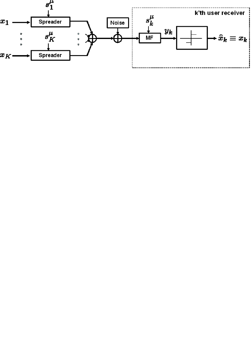
Figure 1: Discrete-time schematic of the complexity-constrained CDMA downlink.

We want to convey information reliably through the channel (1) under a low-complexity constraint on the user receiver. According to this constraint, detected bits, $\hat{x}_{k}$, obtained by performing hard decisions directly on the single-user matched filter output samples, must be the same as the transmitted bits. Explicitly,

$$x_{k}\equiv\hat{x}_{k}=\emph{{{Sign}}}(y_{k}),$$ (2)

where $\textrm{Sign}(\cdot)$ is the trivial sign function.

For any $x_{k}$ and $y_{k}$ which maintain the constraint (2), there is a certain positive scalar $\lambda_{k}$ for which

$$x_{k}y_{k}=\lambda_{k}>0.$$ (3)

Moreover, the bounded noise assumption yields that

$$x_{k}\big{(}x_{k}+\sum_{i\neq k}\rho_{ki}x_{i})\big{)}>\kappa,$$ (4)

or alternatively

$$\sum_{i\neq k}\rho_{ki}x_{k}x_{i}>\kappa-1.$$ (5)

It is important to notice that due to the trivial receiver scheme adopted, and especially its non-linear sign operation, the Shannon capacity becomes invariant in the exact noise probability distribution function, but it only depends on the noise upper and lower values $\pm\kappa\sqrt{P}$. This explains why the bounded noise definition, regardless of its exact probability distribution function form, suffices.

Under the constraints outlined above it is clear that not all combinations of input symbols will result in errorless communication. Thus, the capacity of the channel can be obtained by evaluating the number of codewords that ensure errorless detection. The codewords constraint (5) is analogous to the constraint on the single-neuron (or spin) flip metastable states of the Hopfield model. In the following section we prove that this complexity-constrained CDMA channel setting yields non-trivial capacity.

3 Asymptotic Capacity

A binary codeword ${\bf x}^{c}\triangleq\{x_{1}^{c},\ldots,x_{K}^{c}\}$, composed of all $K$ users’ bits at a given channel use, for which the channel constraints (5) hold, satisfies the condition

$$\int_{\kappa-1}^{\infty}\prod_{k=1}^{K}d\lambda_{k}\delta(\sum_{i\neq k}\rho_{ki}x_{i}-\lambda_{k}x_{k})=1.$$ (6)

Condition (6) can be reformulated as

$$\alpha\int_{\kappa-1}^{\infty}\prod_{k=1}^{K}d\lambda_{k}\delta(\sum_{i\neq k}\alpha\rho_{ki}x_{i}-\alpha\lambda_{k}x_{k})$$

$$= \int_{\alpha(\kappa-1)}^{\infty}\prod_{k=1}^{K}d\lambda_{k}\delta(\sum_{i\neq k}\alpha\rho_{ki}x_{i}-\lambda_{k}x_{k})=1.$$

Let the random variable $\mathbb{N}(K,\beta,\rho,\kappa)$ denote the number of codewords, i.e.

$$\mathbb{N}(K,\beta,\rho,\kappa)\triangleq\\ \int_{\alpha(\kappa-1)}^{\infty}\prod_{k=1}^{K}d\lambda_{k}\delta(\sum_{i\neq k}\alpha\rho_{ki}x_{i}-\lambda_{k}x_{k}).$$ (8)

Assuming equal user information rates, the corresponding asymptotic capacity of the channel is defined [9], in bit information units, as

$$C_{\infty}(\beta,\kappa)\triangleq\lim_{K\rightarrow\infty}\frac{\log_{2}{\mathbb{N}(K,\beta,\rho,\kappa)}}{K}.$$ (9)

Assuming self-averaging property [2, 10], in the large-system limit $K\rightarrow\infty$ the number of successful codewords $\mathbb{N}(K,\beta,\rho,\kappa)$ is equal to its expectation w.r.t. the distribution of $\rho$, i.e.

$$\lim_{K\rightarrow\infty}\mathbb{N}(K,\beta,\rho,\kappa)=\mathcal{N}(\beta,\kappa)$$ (10)

$$= \lim_{K\rightarrow\infty}\int_{\alpha(\kappa-1)}^{\infty}\prod_{k}d\lambda_{k}\sum_{{\bf x}}\Bigg{<}\prod_{k}\delta\Big{(}\sum_{i\neq k}\alpha\rho_{ki}x_{i}-\lambda_{k}x_{k}\Big{)}\Bigg{>}_{\rho},$$

where $\mathcal{N}(\beta,\kappa)$ denotes the average.

Representing the delta function by the inverse Fourier transform of an exponent, expression (10) can be rewritten as

$$\mathcal{N}(\beta,\kappa) = \lim_{K\rightarrow\infty}\int_{\alpha(\kappa-1)}^{\infty}\prod_{k}d\lambda_{k}\frac{1}{(2\pi)^{K}}\int_{-\infty}^{\infty}\prod_{k}d\omega_{k}$$ (11)

$$\times \sum_{{\bf x}}\exp{\Big{(}j\sum_{k}{\omega_{k}\lambda_{k}x_{k}}\Big{)}}\Bigg{<}\exp{\Big{(}-j\sum_{i\neq k}\alpha\rho_{ki}x_{i}\omega_{k}\Big{)}}\Bigg{>}_{\rho}.$$

Substituting $x_{k}\omega_{k}$ for $\omega_{k}$, we find

$$\mathcal{N}(\beta,\kappa) = \lim_{K\rightarrow\infty}\int_{\alpha(\kappa-1)}^{\infty}\prod_{k}d\lambda_{k}\frac{1}{(2\pi)^{K}}\int_{-\infty}^{\infty}\prod_{k}d\omega_{k}$$ (12)

$$\times \sum_{{\bf x}}\exp{\Big{(}j\sum_{k}{\omega_{k}\lambda_{k}}\Big{)}}\cdot\mathbb{E},$$

where

$$\mathbb{E} \triangleq \Bigg{<}\exp{\Big{(}-j\sum_{i\neq k}\alpha\rho_{ki}x_{i}x_{k}\omega_{k}\Big{)}}\Bigg{>}_{\rho}$$ (13)

$$= \Bigg{<}\exp{\Big{(}-j\sum_{i\neq k}\frac{1}{K}\sum_{\mu=1}^{N}s_{k}^{\mu}s_{i}^{\mu}x_{i}x_{k}\omega_{k}\Big{)}}\Bigg{>}_{\rho}.$$

The expectation $\mathbb{E}$ can be also written as

$$\mathbb{E} = \exp{(j\alpha\sum_{k}\omega_{k})}\Bigg{<}\exp{\Big{(}-\frac{j}{K}\sum_{\mu}(\sum_{k}s_{k}^{\mu}x_{k}\omega_{k})(\sum_{k}s_{k}^{\mu}x_{k})\Big{)}}\Bigg{>}_{\rho}.$$ (14)

Using the transformation [11]

$$\exp{(-jA_{\mu}B_{\mu}/K)} = \int_{-\infty}^{\infty}\frac{da_{\mu}}{(2\pi/K)^{1/2}}\int_{-\infty}^{\infty}\frac{db_{\mu}}{(2\pi/K)^{1/2}}$$

$$\times \exp{\Big{(}j\frac{K}{2}(a_{\mu}^{2}-b_{\mu}^{2})-\frac{j}{\sqrt{2}}A_{\mu}(a_{\mu}+b_{\mu})-\frac{j}{\sqrt{2}}B_{\mu}(a_{\mu}-b_{\mu})\Big{)}},$$

expression (14) becomes (here, and hereafter, logarithms are taken to base $e$)

$$\mathbb{E} = \exp{(j\alpha\sum_{k}\omega_{k})}\int_{-\infty}^{\infty}\prod_{\mu}\frac{da_{\mu}}{(2\pi/K)^{1/2}}\int_{-\infty}^{\infty}\prod_{\mu}\frac{db_{\mu}}{(2\pi/K)^{1/2}}$$ (16)

$$\times \exp{\Big{(}j\frac{K}{2}\sum_{\mu}(a_{\mu}^{2}-b_{\mu}^{2})+\sum_{k,\mu}\log\big{(}\cos(c_{k,\mu})\big{)}\Big{)}},$$

where

$$c_{k,\mu}\triangleq\frac{1}{\sqrt{2}}\big{(}\omega_{k}(a_{\mu}+b_{\mu})+(a_{\mu}-b_{\mu})\big{)}.$$ (17)

Since $\sum_{k}s_{k}^{\mu}x_{k}$ in (14) is $\mathcal{O}(\sqrt{K})$ for a vast majority of codewords, for the expectation $\mathbb{E}$ to be finite, $a_{\mu}$ and $b_{\mu}$ must be $\mathcal{O}(1/\sqrt{K})$. Hence, expanding the $\log\big{(}\cos(\cdot)\big{)}$ term in exponent (16) and neglecting terms of order $1/K$ and higher, we get

$$\mathbb{E} = \exp{(j\alpha\sum_{k}\omega_{k})}\int_{-\infty}^{\infty}\prod_{\mu}\frac{da_{\mu}}{(2\pi/K)^{1/2}}\int_{-\infty}^{\infty}\prod_{\mu}\frac{db_{\mu}}{(2\pi/K)^{1/2}}$$ (18)

$$\times \exp{\Big{(}j\frac{K}{2}\sum_{\mu}(a_{\mu}^{2}-b_{\mu}^{2})-\frac{1}{4}\sum_{k,\mu}\hat{c}_{k,\mu}\Big{)}},$$

where

$$\hat{c}_{k,\mu}\triangleq\big{(}\omega_{k}^{2}(a_{\mu}+b_{\mu})^{2}+2\omega_{k}(a_{\mu}^{2}-b_{\mu}^{2})+(a_{\mu}-b_{\mu})^{2}\big{)}.$$ (19)

Now, the solution of the $K$-dimensional integral (18) of the expectation $\mathbb{E}$ is performed using the following mathematical recipe: New variables are introduced

$$a \triangleq \frac{1}{2\alpha}\sum_{\mu}(a_{\mu}+b_{\mu})^{2},$$ (20)

$$b \triangleq \frac{j}{2\alpha}\sum_{\mu}(a_{\mu}^{2}-b_{\mu}^{2})+1.$$ (21)

Equations (20) and (21) can be reformulated via the integral representation of a delta function using the corresponding angular frequencies $A$ and $B$, respectively,

$$\int_{-\infty}^{\infty}\frac{da\,dA}{2\pi/K\alpha}\exp{\big{(}jKA(\alpha a-\sum_{\mu}\frac{(a_{\mu}+b_{\mu})^{2}}{2})\big{)}} = 1,$$ (22)

$$\int_{-\infty}^{\infty}\frac{db\,dB}{2\pi/K\alpha}\exp{\big{(}jKB(\alpha b-j\sum_{\mu}\frac{(a_{\mu}^{2}-b_{\mu}^{2})}{2}-\alpha)\big{)}} = 1.$$ (23)

Substituting these (unity) integrals into the expectation expression (18) and rewriting it using $a$ and $b$, the integrations over $a_{\mu}$ and $b_{\mu}$ are decoupled and can be performed easily. Next, for the asymptotics $K\rightarrow\infty$, the integration over the frequencies $A$ and $B$ can be performed algebraically by the saddle-point method [10].

According to this method, the main contribution to the integral comes from values of $A$ and $B$ in the vicinity of the maximum of the exponent’s argument. Finally, the $\mathbb{E}$ term boils down to

$$\mathbb{E} = \int_{-\infty}^{\infty}\frac{da\ db}{4\pi/K\alpha}\exp{\big{(}-\frac{1}{2}\alpha a\sum_{k}\omega_{k}^{2}+j\alpha b\sum_{k}\omega_{k}\big{)}}$$ (24)

$$\times \exp{\big{(}K\alpha(b-\frac{1}{2}+\frac{(1-b)^{2}}{2a}+\frac{1}{2}\log{a})\big{)}}.$$

Substituting the expectation term (24) back in (12), the integrand in the latter becomes independent of ${\bf x}$, and therefore the $\sum_{{\bf x}}$ can be substituted by multiplying with the scalar $2^{K}$. Hence,

$$\mathcal{N}(\beta,\kappa) = \lim_{K\rightarrow\infty}\int_{\alpha(\kappa-1)}^{\infty}\prod_{k}d\lambda_{k}\frac{1}{\pi^{K}}\int_{-\infty}^{\infty}\prod_{k}d\omega_{k}\exp{\Big{(}j\sum_{k}{\omega_{k}\lambda_{k}}\Big{)}}$$ (25)

$$\times \int_{-\infty}^{\infty}\frac{da\ db}{4\pi/K\alpha}\exp{\Big{(}K\alpha\big{(}b-\frac{1}{2}+\frac{(1-b)^{2}}{2a}+\frac{1}{2}\log{a}\big{)}\Big{)}}$$

$$\times \exp{\Big{(}-\frac{1}{2}\alpha a\sum_{k}\omega_{k}^{2}+j\alpha b\sum_{k}\omega_{k}\Big{)}},$$

where the resulting $\omega$ dependent integrand is a Gaussian function. Thus, performing Gaussian integration and exploiting the symmetry in the $K$-dimensional space, we get

$$\mathcal{N}(\beta,\kappa) = \lim_{K\rightarrow\infty}\frac{1}{\pi^{K}}\int_{-\infty}^{\infty}\frac{da\ db}{4\pi/K\alpha}\exp{\Big{(}K\alpha\big{(}b-\frac{1}{2}+\frac{(1-b)^{2}}{2a}+\frac{1}{2}\log{a}\big{)}\Big{)}}$$ (26)

$$\times \exp{\bigg{(}K\log{\Big{(}\sqrt{\frac{2\pi}{\alpha a}}\int_{\alpha(\kappa-1)}^{\infty}d\lambda\exp{\big{(}-\frac{(\alpha b+\lambda)^{2}}{2\alpha a}\big{)}}\Big{)}}\bigg{)}}.$$

Using the rescaling $(\alpha b+\lambda)/\sqrt{\alpha a}\rightarrow\lambda$, the integral (26) becomes

$$\mathcal{N}(\beta,\kappa)=\lim_{K\rightarrow\infty}\int_{-\infty}^{\infty}\frac{da\ db}{4\pi/K\alpha}\exp{\big{(}Kg(a,b,\beta,\kappa)\big{)}},$$ (27)

where the function $g(a,b,\beta,\kappa)$ is defined by

$$g(a,b,\beta,\kappa)\triangleq\frac{1}{\beta}\big{(}b-\frac{1}{2}+\frac{(1-b)^{2}}{2a}+\frac{1}{2}\log{a}\big{)}+\log\big{(}2Q(t)\big{)},$$ (28)

with an auxiliary variable

$$t\triangleq\frac{\sqrt{\alpha}(b+\kappa-1)}{\sqrt{a}}.$$ (29)

Again, for $K\rightarrow\infty$, the double integral in (27) can be evaluated by the saddle-point method. Hence, we find

$$\mathcal{N}(\beta,\kappa)\propto\lim_{K\rightarrow\infty}\exp{\big{(}Kg(a^{\ast},b^{\ast},\beta,\kappa)\big{)}},$$ (30)

where $a^{\ast}$ and $b^{\ast}$ are found by the saddle-point conditions, which yield the following equations

$$\frac{\partial g(a,b,\beta,\kappa)}{\partial a} = \beta^{-1}\big{(}\frac{(1-b)^{2}}{a}-1\big{)}+t\frac{Q^{\prime}(t)}{Q(t)}=0,$$ (31)

$$\frac{\partial g(a,b,\beta,\kappa)}{\partial b} = \beta^{-1}\big{(}1-\frac{1-b}{a}\big{)}+\frac{1}{\sqrt{a\beta}}\frac{Q^{\prime}(t)}{Q(t)}=0.$$ (32)

One then finds that this set of equations is satisfied by

$$b^{\ast} = 0,$$ (33)

$$a^{\ast} = \beta^{-1}/\big{(}{\beta^{-1}+\frac{1}{\sqrt{a^{\ast}\beta}}\frac{Q^{\prime}(t^{\ast})}{Q(t^{\ast})}}\big{)},$$ (34)

where

$$t^{\ast}\triangleq(\kappa-1)/{\sqrt{a^{\ast}\beta}}.$$ (35)

This saddle-point condition’s fixed-point $a^{\ast}$ can be found iteratively, and it always converges in the examined model [5].

Finally, substituting (30) into (9) the asymptotic capacity, in nat per symbol per user, is now easily obtained

$$C_{\infty}(\beta,\kappa)=g(a^{\ast},b^{\ast},\beta,\kappa)=\log\big{(}2Q(t^{\ast})\big{)}+\frac{1}{\beta}\big{(}\frac{1}{2a^{\ast}}+\frac{1}{2}\log{a^{\ast}}-\frac{1}{2}\big{)},$$ (36)

which forms our pivotal result. In section 4 we further discuss the theoretical results and compare them with computer simulations of the complexity-constrained CDMA channel.

4 Results and Discussion

Fig. 2 displays the asymptotic capacity $C_{\infty}$ (36), obtained by solving iteratively the saddle-point condition (34), as a function of the load $\beta$ in various noise levels. Interestingly, in noiseless channel ($\kappa=0$) for small $\beta\lesssim 0.1$ values the trivial 1 bit upper bound (of an optimal receiver, i.e. matrix inversion) is practically achieved by this simple hard decision operation.

Furthermore, for higher system load such a complexity-constrained CDMA setting still yields substantial achievable information rates. Note, in passing, that for heavily overloaded system (i.e. $\beta\rightarrow\infty$) the capacity curve decay of the noiseless case coincides with Hopfield model’s capacity (see [4, eq. (12)] for an analytical approximation of this capacity decay to zero.) Even in the presence of noise non-negligible rates are obtained for the examined noise levels (up to $\kappa=1$) in a wide range of load values.

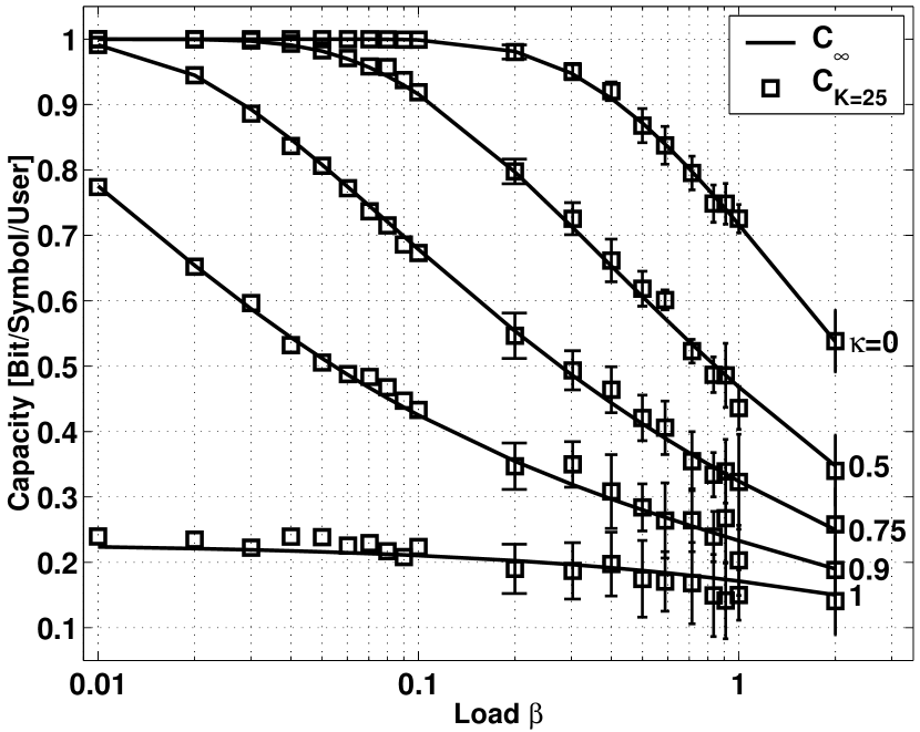
Figure 2: Asymptotic capacity $C_{\infty}$ (solid line), in terms of bit/symbol/user, as a function of load $\beta$ in various noise levels $\kappa=0,0.5,0.75,0.9,1$. Also drawn is the finite-size simulation-averaged capacity $C_{K}$ for $K=25$ (empty squares). Vertical bars stand for standard deviation in simulation results.

In order to validate the analytically derived asymptotic capacity $C_{\infty}(\beta,\kappa)$, we evaluated the capacity $C_{K}(\beta,\kappa)$ of a noisy CDMA downlink channel with large, yet finite number of users $K$, using exhaustive search simulations. The number of successful binary codewords, maintaining the channel constraints (5), was obtained by examining all $2^{K}$ possible codewords. The average logarithm of the counted number, normalized by the number of users $K$, gives the capacity $C_{K}$.

Fig. 2 presents the capacity obtained by simulations for $K=25$. As can be seen, the empirical capacity for finite $K$ deviates only slightly from the analytically obtained asymptotic capacity. Due to finite-size effects these slight deviations from theoretical results grow with the decrease in the capacity. These results substantiate the analysis of the complexity-constrained CDMA channel.

The devised capacity is also drawn in a reciprocal manner. Fig. 3 displays $C_{\infty}$ as a function of the noise threshold $\kappa$, this time for a fixed load $\beta$. The capacity decreases monotonically as a function of $\kappa$ from asymptotically $1$ bit down to zero capacity.

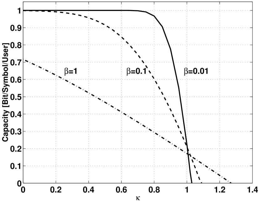
Figure 3: Asymptotic capacity $C_{\infty}$, in terms of bit/symbol/user, as a function of noise levels $\kappa$ for a fixed load $\beta=0.01\,\textrm{(solid line)},0.1\,\textrm{(dashed)},1\,\textrm{(dashdotted)}$.

Three typical regimes can be readily observed: As may be expected, for noise thresholds $\kappa\lesssim 1$, an increase in system load $\beta$ directly results in lower capacity. On the other hand, for thresholds $\kappa\gtrsim 1$, as the system becomes more loaded, the maximum achievable rate increases, and the interfering users play a constructive, rather than destructive role.

This fascinating phenomenon can be explained by the fact that when the noise becomes more dominant (i.e. at the order of information power $P$), a certain user’s designated information bit can not exceed the transmission constraint by itself and needs the assistance of the ”interference” term (organized properly) in order to deliver its own information reliably.

For $\beta=0.01$, $0.1$ and $1$ zero capacity is found to be inevitable starting from noise thresholds $\approx 1.05$, $1.09$ and $1.27$, respectively, for which reliable communication in this complexity-constrained setting becomes infeasible. The transition between these two regimes occurs at the vicinity of $\kappa=1$, for which the capacity is approximately $0.2$ bit, regardless of the examined system load (as can be seen more clearly from Fig. 2.)

4.1 AWGN and Outage Capacity

Evidently, for unbounded noise distribution, like the popular additive white Gaussian noise (AWGN), Shannon capacity, under the examined complexity constraint, is zero. However, the analysis is still useful for obtaining the outage capacity instead of the Shannon capacity.

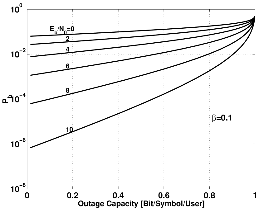
Figure 4: Outage capacity for AWGN: bit error rate per user $P_{b}$ as a function of the rate, in terms of bit/symbol/user, for various $E_{b}/N_{0}$ levels ($\beta=0.1$).

Fig. 4 presents the bit error rate (BER) per user $P_{b}$ as a function of the corresponding outage capacity, in terms of bit/symbol/user, for different signal-to-noise ratios in the case of AWGN. The BER is evaluated by computing the probability $\Pr(n_{k}>\kappa\sqrt{P})$, and then it is linked to a certain achievable information rate via the analytically derived capacity-threshold dependency (e.g. the curves in Fig. 3). It can be seen that reasonable information rates can be achieved.

For instance, for $E_{b}/N_{0}=10$dB a BER of 0.001 (which is the BER typically required for voice traffic) can be reached with a rate of 0.75 bit. For comparison, without any complexity constraint the Shannon capacity for binary-input AWGN CDMA is asymptotically 1 bit [2]. However, in order to approach this capacity an optimal multiuser receiver with intractable complexity of $\mathcal{O}(2^{K})$ is required, along with a sophisticated decoding mechanism, while at the cost of 0.25 bit the proposed trivial receiver will do (for voice traffic).

5 Conclusion

We evaluated the asymptotic capacity of a noisy CDMA downlink channel model requiring only minimal signal processing at the receiver, thus suitable for networks with low-complexity mobile equipment. Interestingly, we found a range of non-trivial achievable rates.

According to these findings, at a given channel use a fraction of the users, equal to $C_{\infty}$ (in bit), can receive its designated information with rate $1$, while the transmissions to the rest of the users ensure reliable communication. Determining these redundant transmissions in a diagrammatic manner (rather than via brute-force enumeration, which becomes infeasible for large $K$) remains an interesting open research question. Also, the method used can be employed in the investigation of other (non-CDMA) noisy complexity-constrained channels.

References

- [1] S. Verdú, and S. Shamai (Shitz), “Spectral Efficiency of CDMA with Random Spreading,” IEEE Trans. Inform. Theory, vol. 45, no. 2, pp. 622–640, Mar. 1999.
- [2] T. Tanaka, “A statistical-mechanics approach to large-system analysis of CDMA multiuser detectors,” IEEE Trans. Inform. Theory, vol. 48, pp. 2888–2910, Nov. 2002.
- [3] O. Shental, I. Kanter, and A. J. Weiss, “Capacity of Complexity-Constrained Noise-Free CDMA,” to appear in IEEE Communications Letters.
- [4] E. J. Gardner, “Structure of Metastable States in the Hopfield Model,” J. Phys. A: Math. Gen., vol. 19, pp. L1047–L1052, 1986.
- [5] M. P. Singh, “Hopfield Model with Self-Coupling,” Phys. Rev. A, vol. 64, p. 051912, 2001.
- [6] G. I. Kechriotis, and E. S. Manolakos, “Hopfield neural network implementation of the optimal CDMA multiuser detector,” IEEE Trans. Neural Networks, vol. 7, pp. 131–141, 1996.
- [7] T. Tanaka, “Analysis of bit error probability of direct-sequence CDMA multiuser demodulators,” in Advances in Neural Information Processing Systems, T. Leen, T. Dietterich, and V. Tresp, Eds. Cambridge, MA: MIT Press, 2001, vol. 13, pp. 315 -321.
- [8] ——, “Statistical mechanics of CDMA multiuser demodulation,” in Europhys. Lett., vol. 54, no. 4, pp. 540 -546, 2001.
- [9] T. M. Cover and J. A. Thomas, Elements of Information Theory. John Wiley and Sons, 1991.
- [10] R. S. Ellis, Entropy, Large Deviations, and Statistical Mechanics. Springer-Verlag, 1985.
- [11] A. D. Bruce, E. J. Gardner and D. J. Wallace, “Dynamics and Statistical Mechanics of the Hopfield Model,” J. Phys. A: Math. Gen., vol. 20, pp. 2909–2934, 1987.