Capacity of Complexity-Constrained
Noise-Free CDMA

Abstract

An interference-limited noise-free CDMA downlink channel operating under a complexity constraint on the receiver is introduced. According to this paradigm, detected bits, obtained by performing hard decisions directly on the channel’s matched filter output, must be the same as the transmitted binary inputs. This channel setting, allowing the use of the simplest receiver scheme, seems to be worthless, making reliable communication at any rate impossible. We prove, by adopting statistical mechanics notion, that in the large-system limit such a complexity-constrained CDMA channel gives rise to a non-trivial Shannon-theoretic capacity, rigorously analyzed and corroborated using finite-size channel simulations.

I Introduction

Direct-sequence spread-spectrum code-division multiple-access (CDMA) is used extensively in modern wireless communication systems and serves preeminently in commercial cellular networks. Investigation of reliable (i.e. errorless) communication via the CDMA channel is a long-standing and productive research topic (e.g., [1]).

A typical investigation of a CDMA channel often assumes an upper bounded transmission power, but no restrictions on complexity are imposed. In the era of ubiquitous and pervasive communications, in, for example, indoor and personal area networks (PAN), there is an emerging interest in a complementary scenario. According to this scenario, the CDMA system operates in a high signal-to-noise ratio (SNR) regime (thus power limitation is less crucial), but is highly restricted by its receiver’s signal processing complexity. For instance, this is the case in complexity-limited (rather than noise-limited) CDMA downlink, where the simplest mobile receiver is to be used. Such a trivial receiver requires that detected bits, sliced at the output of the channel’s matched filter, must be the same as the transmitted binary inputs. Formerly, there has been no examination of the information-theoretic characteristics of CDMA channels in this setting, being especially applicable for the downlink.

In this contribution, we compute the Shannon capacity of such a complexity-constrained CDMA channel with binary signaling, random spreading and arbitrary user load. For this purpose, we borrow analysis tools from equilibrium statistical mechanics, especially the Hopfield model of neural networks [2, 3]. The achievable asymptotic information rates of such naive CDMA channels, which may seem worthless from an information-theoretic point of view, are found to result in valuable rates, comparable to those achieved by using the optimal multi-user receiver.

II Channel Model

Consider a noiseless synchronous CDMA downlink accessing $K$ active users via the mutual channel in order to transmit their designated (coded) information binary symbols, $x_{k}=\pm 1$, where $k=1,\ldots,K$. Each transmission to a user is assigned with a binary signature sequence (spreading code) of $N$ chips, $s_{k=1\ldots K}^{\mu=1\ldots N}=\pm 1$. Assuming a random spreading model, the binary chips are independently equiprobably chosen, and the deterministic chip waveform has unit energy. The cross-correlation between users’ transmissions is $\rho_{ki}\triangleq 1/N\sum_{\mu}s_{k}^{\mu}s_{i}^{\mu}$. The received signal is passed through the user’s matched filter. Thus, the overall channel input-output relation is described by

$$y_{k}=x_{k}+\sum_{i\neq k}\rho_{ki}x_{i},$$ (1)

where the $k$’th user matched filter output, $y_{k}$, is the designated bit, $x_{k}$, corrupted by an interference term. This interference term is composed of a summation over (cross-correlation) scaled versions of all other users’ bits. The set of all cross-correlations $\rho_{ki}$ is hereinafter denoted by $\rho$. In the following asymptotic analysis, we assume that $K\rightarrow\infty$, yet the system load factor $\beta\triangleq K/N\triangleq\alpha^{-1}$ is kept constant, and that the information rate is the same for all users, i.e. $R_{k}=R$.

We want to convey information reliably through the channel (1) under a low-complexity constraint on the user receiver. According to this constraint, detected bits, $\hat{x}_{k}$, obtained by performing hard decisions directly on the channel’s matched filter output samples, must be the same as the transmitted bits. Explicitly, $x_{k}\equiv\hat{x}_{k}=\emph{{{Sign}}}(y_{k})$, where $\textrm{Sign}(\cdot)$ is the trivial sign function. Under the constraints outlined above it is clear that not all combinations of input symbols will result in errorless communication. Thus, the capacity of the channel can be obtained by evaluating the number of codewords that ensure errorless detection. Following, we prove that this complexity-constrained CDMA channel setting yields non-trivial capacity.

III Capacity

A binary codeword ${\bf x}^{c}\triangleq\{x_{1}^{c},\ldots,x_{K}^{c}\}$, composed of all $K$ users’ bits at a given channel use, for which the channel constraints hold, satisfies the condition

$$\int_{0}^{\infty}\prod_{k=1}^{K}d\lambda_{k}\delta(y_{k}-\lambda_{k}x_{k}^{c})=\int_{0}^{\infty}\prod_{k=1}^{K}d\lambda_{k}\delta(\alpha y_{k}-\lambda_{k}x_{k}^{c})=1,$$

where $\delta(\cdot)$ is the Dirac delta function. Let the random variable $\mathbb{N}(K,\beta,\rho)$ denote the number of codewords, i.e.

$$\mathbb{N}(K,\beta,\rho)\triangleq\int_{-\alpha}^{\infty}\prod_{k}d\lambda_{k}\sum_{{\bf x}}\prod_{k}\delta\Big{(}\sum_{i\neq k}\alpha\rho_{ki}x_{i}-\lambda_{k}x_{k}\Big{)},$$

where $\sum_{{\bf x}}$ corresponds to a sum over all the possible values of the transmitted input symbols. Assuming equal user information rates, the corresponding asymptotic capacity of the channel is defined [4], in bit information units, as $C_{\infty}(\beta)\triangleq\lim_{K\rightarrow\infty}\log_{2}{\mathbb{N}(K,\beta,\rho)}/K$. According to the self-averaging property [5], in the large-system limit, $K\rightarrow\infty$, the number of successful codewords $\mathbb{N}(K,\beta,\rho)$ is equal to its expectation with respect to (w.r.t.) the distribution of $\rho$, i.e.

$$\lim_{K\rightarrow\infty}\mathbb{N}(K,\beta,\rho) = \mathcal{N}(\beta)=\lim_{K\rightarrow\infty}\int_{-\alpha}^{\infty}\prod_{k}d\lambda_{k}$$

$$\times \sum_{{\bf x}}\Bigg{<}\prod_{k}\delta\Big{(}\sum_{i\neq k}\alpha\rho_{ki}x_{i}-\lambda_{k}x_{k}\Big{)}\Bigg{>}_{\rho},$$

where $\mathcal{N}(\beta)$ and $<\cdot>_{\rho}$ denote the average and averaging operation, respectively. Representing the delta function by the inverse Fourier transform of an exponent and substituting $x_{k}\omega_{k}$ for the angular frequency of the Fourier transform $\omega_{k}$, expression (III) can be rewritten as

$$\mathcal{N}(\beta) = \lim_{K\rightarrow\infty}\int_{-\alpha}^{\infty}\prod_{k}d\lambda_{k}\frac{1}{(2\pi)^{K}}\int_{-\infty}^{\infty}\prod_{k}d\omega_{k}$$ (3)

$$\times \sum_{{\bf x}}\exp{\Big{(}j\sum_{k}{\omega_{k}\lambda_{k}}\Big{)}}\cdot\mathbb{E},$$

where $j\triangleq\sqrt{-1}$ and

$$\mathbb{E}\triangleq\Bigg{<}\exp{\Big{(}-j\sum_{i\neq k}\frac{1}{K}\sum_{\mu=1}^{N}s_{k}^{\mu}s_{i}^{\mu}x_{i}x_{k}\omega_{k}\Big{)}}\Bigg{>}_{\rho}.$$

The expectation $\mathbb{E}$ can be also written as

$$\mathbb{E} = \exp{(j\alpha\sum_{k}\omega_{k})}$$ (4)

$$\times \Big{<}\exp{\big{(}-\frac{j}{K}\sum_{\mu}(\sum_{k}s_{k}^{\mu}x_{k}\omega_{k})(\sum_{k}s_{k}^{\mu}x_{k})\big{)}}\Big{>}_{\rho}.$$

Using a transformation [6, eq. (2.14)], the expectation becomes

$$\mathbb{E} = \exp{(j\alpha\sum_{k}\omega_{k})}\int_{-\infty}^{\infty}\prod_{\mu}\frac{da_{\mu}}{(2\pi/K)^{1/2}}$$ (5)

$$\times \int_{-\infty}^{\infty}\prod_{\mu}\frac{db_{\mu}}{(2\pi/K)^{1/2}}\exp{\Big{(}j\frac{K}{2}\sum_{\mu}(a_{\mu}^{2}-b_{\mu}^{2})\Big{)}}$$

$$\times \exp{\Big{(}\sum_{k,\mu}\log\big{(}\cos(c_{k,\mu})\big{)}\Big{)}},$$

where $c_{k,\mu}\triangleq\frac{1}{\sqrt{2}}\big{(}\omega_{k}(a_{\mu}+b_{\mu})+(a_{\mu}-b_{\mu})\big{)}$. Since $\sum_{k}s_{k}^{\mu}x_{k}$ in (4) is $\mathcal{O}(\sqrt{K})$ for an overwhelming majority of codewords, for the expectation $\mathbb{E}$ to be finite, $a_{\mu}$ and $b_{\mu}$ must be $\mathcal{O}(1/\sqrt{K})$. Hence, expanding the $\log\big{(}\cos(\cdot)\big{)}$ term in exponent (5) and neglecting terms of order $1/K$ and higher, we get

$$\mathbb{E} = \exp{(j\alpha\sum_{k}\omega_{k})}\int_{-\infty}^{\infty}\prod_{\mu}\frac{da_{\mu}}{(2\pi/K)^{1/2}}$$ (6)

$$\times \int_{-\infty}^{\infty}\prod_{\mu}\frac{db_{\mu}}{(2\pi/K)^{1/2}}\exp{\Big{(}j\frac{K}{2}\sum_{\mu}(a_{\mu}^{2}-b_{\mu}^{2})\Big{)}}$$

$$\times \exp{\Big{(}-\frac{1}{4}\sum_{k,\mu}\hat{c}_{k,\mu}\Big{)}},$$

where $\hat{c}_{k,\mu}\triangleq\big{(}\omega_{k}^{2}(a_{\mu}+b_{\mu})^{2}+2\omega_{k}(a_{\mu}^{2}-b_{\mu}^{2})+(a_{\mu}-b_{\mu})^{2}\big{)}$. Now, the multi-dimensional integral (6) is solved using the following mathematical recipe: New variables are introduced

$$a\triangleq\frac{1}{2\alpha}\sum_{\mu}(a_{\mu}+b_{\mu})^{2},\quad b\triangleq\frac{j}{2\alpha}\sum_{\mu}(a_{\mu}^{2}-b_{\mu}^{2})+1.$$ (7)

Equations (7) can be reformulated via the integral representation of a delta function using the corresponding angular frequencies $A$ and $B$, respectively,

$$\int_{-\infty}^{\infty}\frac{da\ dA}{2\pi/K\alpha}\exp{\big{(}jKA(\alpha a-\sum_{\mu}\frac{(a_{\mu}+b_{\mu})^{2}}{2})\big{)}}=1,$$

$$\int_{-\infty}^{\infty}\frac{db\ dB}{2\pi/K\alpha}\exp{\big{(}jKB(\alpha b-j\sum_{\mu}\frac{(a_{\mu}^{2}-b_{\mu}^{2})}{2}-\alpha)\big{)}}=1.$$

Substituting these (unity) integrals into the expectation expression (6) and rewriting it using $a$ and $b$, the integrations over $a_{\mu}$ and $b_{\mu}$ are decoupled and can be performed easily. Next, for the asymptotics $K\rightarrow\infty$, the integration over the frequencies $A$ and $B$ can be performed algebraically by the saddle-point method [5]. According to this method, the main contribution to the integral comes from values of $A$ and $B$ in the vicinity of the maximum of the exponent’s argument. Finally, the $\mathbb{E}$ term boils down to

$$\mathbb{E} = \int_{-\infty}^{\infty}\frac{da\ db}{4\pi/K\alpha}\exp{\big{(}K\alpha(b-\frac{1}{2}+\frac{(1-b)^{2}}{2a}+\frac{1}{2}\log{a})\big{)}}$$ (8)

$$\times \exp{\big{(}-\frac{1}{2}\alpha a\sum_{k}\omega_{k}^{2}+j\alpha b\sum_{k}\omega_{k}\big{)}}.$$

Substituting the expectation term (8) back in (3), the integrand in the latter becomes independent of ${\bf x}$, therefore the $\sum_{{\bf x}}$ can be substituted by multiplying with the scalar $2^{K}$, and the resulting $\omega$ dependent integrand is a Gaussian function. Thus performing Gaussian integration and exploiting the symmetry in the $K$-dimensional space, we get

$$\mathcal{N}(\beta)=\lim_{K\rightarrow\infty}\frac{1}{\pi^{K}}\int_{-\infty}^{\infty}\frac{da\ db}{4\pi/K\alpha}$$

$$\times \exp{\Big{(}K\alpha\big{(}b-\frac{1}{2}+\frac{(1-b)^{2}}{2a}+\frac{1}{2}\log{a}\big{)}\Big{)}}$$

$$\times \exp{\bigg{(}K\log{\Big{(}\sqrt{\frac{2\pi}{\alpha a}}\int_{-\alpha}^{\infty}d\lambda\exp{\big{(}-\frac{(\alpha b+\lambda)^{2}}{2\alpha a}\big{)}}\Big{)}}\bigg{)}}.$$

Using the rescaling $(\alpha b+\lambda)/\sqrt{\alpha a}\rightarrow\lambda$, the integral (III) becomes

$$\mathcal{N}(\beta)=\lim_{K\rightarrow\infty}\int_{-\infty}^{\infty}\frac{da\ db}{4\pi/K\alpha}\exp{\big{(}Kg(a,b,\beta)\big{)}},$$ (10)

where the function $g(a,b,\beta)$ is defined by

$$g(a,b,\beta) \triangleq \frac{1}{\beta}\big{(}b-\frac{1}{2}+\frac{(1-b)^{2}}{2a}+\frac{1}{2}\log{a}\big{)}$$

$$+ \log\big{(}2Q(t)\big{)}.$$

The definitions of the auxiliary variable $t\triangleq\sqrt{\alpha}(b-1)/\sqrt{a}$ and the error function $Q(x)\triangleq 1/\sqrt{2\pi}\int_{x}^{\infty}dy\exp{(-y^{2}/2)}$ are used. Again, for $K\rightarrow\infty$, the double integral in (10) can be evaluated by the saddle-point method. Hence, we find

$$\mathcal{N}(\beta)\propto\lim_{K\rightarrow\infty}\exp{\big{(}Kg(a^{\ast},b^{\ast},\beta)\big{)}},$$ (11)

where $a^{\ast}$ and $b^{\ast}$ are found by the saddle-point conditions, which yield the following equations

$$\frac{\partial g(a,b,\beta)}{\partial a} = \beta^{-1}\big{(}\frac{(1-b)^{2}}{a}-1\big{)}+t\frac{Q^{\prime}(t)}{Q(t)}=0,$$

$$\frac{\partial g(a,b,\beta)}{\partial b} = \beta^{-1}\big{(}1-\frac{1-b}{a}\big{)}+\frac{1}{\sqrt{a\beta}}\frac{Q^{\prime}(t)}{Q(t)}=0.$$

The operator $Q^{\prime}$ denotes a derivative of $Q$ w.r.t. its argument. One then finds that this set of equations is satisfied by $b^{\ast}=0$ and

$$a^{\ast}=\beta^{-1}/\big{(}{\beta^{-1}+\frac{1}{\sqrt{a^{\ast}\beta}}\frac{Q^{\prime}(t^{\ast})}{Q(t^{\ast})}}\big{)},$$ (12)

where $t^{\ast}\triangleq-1/{\sqrt{a^{\ast}\beta}}$. This saddle-point condition’s fixed-point $a^{\ast}$ can be found iteratively, and it always converges in the examined model [3].

Finally, substituting (11) the asymptotic capacity, in nat per symbol per user, is now easily obtained

$$C_{\infty}(\beta) = g(a^{\ast},b^{\ast},\beta)=\log\big{(}2Q(t^{\ast})\big{)}$$ (13)

$$+ \frac{1}{\beta}\big{(}b^{\ast}-\frac{1}{2}+\frac{(1-b^{\ast})^{2}}{2a^{\ast}}+\frac{1}{2}\log{a^{\ast}}\big{)},$$

which forms our pivotal result. In section IV we further discuss the theoretical results and compare them with computer simulations of the complexity-constrained CDMA channel.

IV Results

Fig. 1 displays the asymptotic capacity $C_{\infty}$ (13), obtained by solving iteratively the saddle-point condition (12), as a function of the load $\beta$. Interestingly, for small $\beta\lesssim 0.1$ values the trivial 1 bit upper bound (of an optimal receiver, i.e. matrix inversion) is practically achieved by this simple hard decision operation. Nevertheless, even for higher non-trivial system load such a complexity-constrained CDMA setting still yields substantial achievable information rates. Note, in passing, that for heavily overloaded system (i.e. $\beta\rightarrow\infty$) the capacity curve decay coincides with Hopfield model’s capacity (see [2, eq. (12)] for an analytical approximation of this capacity decay to zero.)

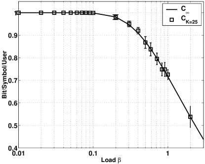
Figure 1: Asymptotic capacity $C_{\infty}$ (solid line), in terms of bit/symbol/user, as a function of load $\beta$. Also drawn is the finite-size simulation-averaged capacity $C_{K}$ for $K=25$ (empty squares). Vertical bars stand for standard deviation in simulation results.

In order to validate the analytically derived asymptotic capacity $C_{\infty}(\beta)$, we evaluated the capacity $C_{K}(\beta)$ of a CDMA downlink channel with large, yet finite number of users $K$, using exhaustive search simulations. The number of successful binary codewords, maintaining the channel constraints, was obtained by examining all $2^{K}$ possible codewords. The average logarithm of the counted number, normalized by the number of users $K$, gives the capacity $C_{K}$. Fig. 1 presents the capacity obtained by simulations for $K=25$. As can be seen, the empirical capacity for finite $K$ deviates only slightly from the analytically obtained asymptotic capacity. These results substantiate the analysis of the complexity-constrained CDMA channel.

V Concluding Remarks

We evaluated the asymptotic capacity of a CDMA downlink channel model requiring only minimal signal processing at the receiver, thus suitable for interference-limited systems with low-complexity constrained mobile equipment. Interestingly, we found a range of non-trivial achievable rates. According to these findings, at a given channel use a fraction of the users, equal to $C_{\infty}$ (in bit), can receive its designated information with rate $1$, while the transmissions to the rest of the users ensure reliable communication. Determining these redundant transmissions in a diagrammatic manner (rather than via brute-force enumeration, which becomes infeasible for large $K$) remains an interesting open research question.

References

• [1] S. Verdú, and S. Shamai (Shitz), “Spectral Efficiency of CDMA with Random Spreading,” IEEE Trans. Inform. Theory, vol. 45, no. 2, pp. 622–640, Mar. 1999.
• [2] E. J. Gardner, “Structure of Metastable States in the Hopfield Model,” J. Phys. A: Math. Gen., vol. 19, pp. L1047–L1052, 1986.
• [3] M. P. Singh, “Hopfield Model with Self-Coupling,” Phys. Rev. A, vol. 64, p. 051912, 2001.
• [4] T. M. Cover and J. A. Thomas, Elements of Information Theory.   John Wiley and Sons, 1991.
• [5] R. S. Ellis, Entropy, Large Deviations, and Statistical Mechanics.   Springer-Verlag, 1985.
• [6] A. D. Bruce, E. J. Gardner and D. J. Wallace, “Dynamics and Statistical Mechanics of the Hopfield Model,” J. Phys. A: Math. Gen., vol. 20, pp. 2909–2934, 1987.