Optimal Power Control for Multiuser
CDMA Channels

Abstract

In this paper, we define the power region as the set of power allocations for $K$ users such that everybody meets a minimum signal-to-interference ratio (SIR). The SIR is modeled in a multiuser CDMA system with fixed linear receiver and signature sequences. We show that the power region is convex in linear and logarithmic scale. It furthermore has a componentwise minimal element. Power constraints are included by the intersection with the set of all viable power adjustments. In this framework, we aim at minimizing the total expended power by minimizing a componentwise monotone functional. If the feasible power region is nonempty, the minimum is attained. Otherwise, as a solution to balance conflicting interests, we suggest the projection of the minimum point in the power region onto the set of viable power settings. Finally, with an appropriate utility function, the problem of minimizing the total expended power can be seen as finding the Nash bargaining solution, which sheds light on power assignment from a game theoretic point of view. Convexity and componentwise monotonicity are essential prerequisites for this result.

I Introduction

In interference limited wireless communication systems, like code division multiple access (CDMA), mobile users regulate transmission power to adapt to varying radio channel and propagation conditions. The main purpose is to minimize interference to other users while maintaining one s own data rate at the lowest possible energy consumption. A number of recent papers is dealing with the intertwining effect of power adjustment and feasible data rates per user in wireless networks, hence defining a concept of overall network capacity, see e.g., [1, 2, 3, 4, 5], and references therein.

A companion problem is the design of efficient power control algorithms, preferably such that each user needs only local information to update his power settings, but global convergence is assured, see [6, 7, 8, 9].

Refined models also include stochastic fading effects of the channel. The usual approach here is to minimize power consumption subject to certain outage probability constraints. Appropriate models, structural properties of the corresponding feasible region, adequate power control algorithms and their convergence are investigated in [6, 10, 11, 12, 13, 14].

In this paper, we investigate properties of the power region and the existence of energy minimal power settings assuming known channel information and fixed signature and linear receiver sequences in CDMA systems. To summarize, the main contributions are as follows.

In Section II we first define the power region for $K$ users as the set of power settings ${\bf 0}\leq\bop\in\mathbb{R}^{K}$, such that in a community of $K$ users each user $i$ encounters a signal-to-noise ratio above a certain threshold $\gamma_{i}$. The power region is shown to be convex in linear and logarithmic scale. It furthermore contains a componentwise minimal element $\bop^{*}$ that can be explicitly determined.

In Section III energy efficient power allocation is formalized as minimizing a componentwise monotone function $h$ over the power region. In practice, however, power is limited. This is included in our model by introducing the feasible power region as the intersection with a convex and downward closed set of viable power adjustments. In the case that there is no feasible power allocation, we suggest the projection of $\bop^{*}$ onto the viable power adjustments as a solution which balances between conflicting interests of users. The solution can be computed by applying cyclic projections onto simple affine subsets.

Finally, by use of an appropriate utility function we show in Section IV how optimal power allocation can be interpreted as a cooperative game. It turns out that the Nash bargaining solution coincides with the solution of the original power minimization problem.

II System Model

In a synchronous multiuser CDMA communication system with $K$ users and processing gain $N$ let $\bos_{i}\in\mathbb{R}^{N}$, $i=1,\ldots,K$, denote the $N$-dimensional signature sequence of user $i$. Let $G_{ij}$ denote the fixed path gain from user $j$ to the assigned base station of user $i$. Usually $G_{ij}$ is subject to slow fading effects which are assumed to be known to the transmitter. Suppose the symbol of user $i$ is decoded using a linear receiver represented by some vector $\boc_{i}\in\mathbb{R}^{N}$. The signal-to-interference ratio of user $i$ is then given as

$${\rm{SIR}}_{i}(\bop)=\frac{G_{ii}(\boc_{i}^{\prime}\bos_{i})^{2}p_{i}}{\sum_{j\not=i}G_{ij}(\boc_{i}^{\prime}\bos_{j})^{2}p_{j}+\sigma^{2}(c_{i}^{\prime}c_{i})^{2}},$$

where $\sigma^{2}$ denotes the variance of the additive Gaussian noise and $\bop=(p_{1},\ldots,p_{K})$ the vector of transmit powers. In the following we assume that the receiver sequences $\boc_{i}$ are fixed. Summarizing the known channel and receiver effects into $A_{ij}=G_{ij}(\boc_{i}^{\prime}\bos_{j})^{2}$ we obtain the following ${\rm{SIR}}_{i}$ of user $i$

$${\rm{SIR}}_{i}(\bop)=\frac{A_{ii}p_{i}}{\sum_{j\not=i}A_{ij}p_{j}+C_{ii}\sigma^{2}}.$$

with $C_{ii}=(\boc_{i}^{\prime}\boc_{i})^{2}$. Now given quality-of-service requirements $\gamma_{1},\ldots,\gamma_{K}$ for each user, we define the power region ${{\cal P}}_{\rm SIR}$ as the set of power settings $\bop\in\mathbb{R}^{K}$ such that each user $i$ meets his minimum SIR requirement $\gamma_{i}$, i.e.,

$${{{\cal P}}_{\rm SIR}}=\big{\{}\bop\geq{\bf 0}\mid{\rm{SIR}}_{i}(\bop)\geq\gamma_{i},\ i=1,\ldots,K\big{\}}.$$ (1)

Here and in the following orderings ’$<$’ and ’$\leq$’ between vectors are always meant componentwise. Obviously it may happen that not all requirements $\gamma_{i}$ can be simultaneously satisfied in which case ${{\cal P}}_{\rm SIR}$ is empty.

We now prove convexity and log-convexity of the power region ${{\cal P}}_{\rm SIR}$. The set ${{\cal P}}_{\rm SIR}$ is called log-convex, if for any $\bop^{(1)},\,\bop^{(2)}\in{{\cal P}}_{\rm SIR}$ and any $0\leq\alpha\leq 1$ the point

$$\bop^{(\alpha)}={\bop^{(1)}}^{\alpha}{\bop^{(2)}}^{1-\alpha}\in{{{\cal P}}_{\rm SIR}},$$

where powers $\bop^{\alpha}=(p_{1}^{\alpha},\ldots,p_{K}^{\alpha})$ are applied componentwise. Taking logarithms componentwise gives

$$\log\bop^{(\alpha)}=\alpha\log{\bop^{(1)}}+(1-\alpha)\log{\bop^{(2)}}$$

which means that the set ${{\cal P}}_{\rm SIR}$ is convex in logarithmic scale.

Proposition 1

The power region ${{\cal P}}_{\rm SIR}$ is convex and log-convex.

Proof.

Consider the sets

$${\cal P}_{i}=\big{\{}\bop\mid A_{ii}p_{i}-\gamma_{i}\sum_{j\not=i}A_{ij}p_{j}\geq\gamma_{i}C_{ii}\sigma^{2}\big{\}},\ i=1,\ldots,K,$$

which are closed convex affine halfspaces in $\mathbb{R}^{K}$. Obviously, ${{\cal P}}_{\rm SIR}=\bigcap_{i=1}^{K}{\cal P}_{i}$, and from Theorem C in section III of [15] it follows that ${{\cal P}}_{\rm SIR}$ is a closed and convex polytope.

To prove log-convexity we show that

$$\begin{split}{\rm{SIR}}_{i}(\bop^{(\alpha)})&\geq\big{(}{\rm{SIR}}_{i}(\bop^{(1)})\big{)}^{\alpha}\big{(}{\rm{SIR}}_{i}(\bop^{(2)})\big{)}^{1-\alpha}\\ &\geq\gamma_{i}^{\alpha}\gamma_{i}^{1-\alpha}=\gamma_{i}\end{split}$$ (2)

for all $i=1,\ldots,K$, which entails $\bop^{(\alpha)}\in{{\cal P}}_{\rm SIR}$. The first inequality in (2) follows from Hölder’s inequality since

$$\sum_{j\not=i}A_{ij}{p_{j}^{(1)}}^{\alpha}{p_{j}^{(2)}}^{1-\alpha}+C_{ii}\sigma^{2}$$

$$\quad\leq\Big{(}\sum_{j\not=i}A_{ij}p_{j}^{(1)}+C_{ii}\sigma^{2}\Big{)}^{\alpha}\Big{(}\sum_{j\not=i}A_{ij}p_{j}^{(2)}+C_{ii}\sigma^{2}\Big{)}^{1-\alpha},$$

hence yielding

$${\rm{SIR}}_{i}\big{(}\bop^{(\alpha)}\big{)}$$

$$\ =\frac{A_{ii}{p_{i}^{(1)}}^{\alpha}{p_{i}^{(2)}}^{1-\alpha}}{\sum_{j\not=i}A_{ij}{p_{i}^{(1)}}^{\alpha}{p_{i}^{(2)}}^{1-\alpha}+C_{ii}\sigma^{2}}$$

$$\ \geq\Big{(}\frac{A_{ii}{p_{i}^{(1)}}}{\sum_{j\not=i}A_{ij}{p_{j}^{(1)}}+C_{ii}\sigma^{2}}\Big{)}^{\alpha}\Big{(}\frac{A_{ii}{p_{i}^{(2)}}}{\sum_{j\not=i}A_{ij}{p_{j}^{(2)}}+C_{ii}\sigma^{2}}\Big{)}^{1-\alpha}$$

$$\ =\big{(}{\rm{SIR}}_{i}(\bop^{(1)})\big{)}^{\alpha}\big{(}{\rm{SIR}}_{i}(\bop^{(2)})\big{)}^{1-\alpha}$$

for all $i=1,\ldots,K$. ∎

III Energy Efficient Power Allocation

For convenience of notation we quote the following result from [3]. It deals with solutions of the equation

$$[\boI-\boA]\boxx=\boc$$ (3)

when $\boA$ is a non-negative but not necessarily irreducible matrix. The proof given in [3] is direct and self-contained, and does not rely on the Perron-Frobenius theory. Let $\rho(\boA)$ denote the spectral radius of a square matrix $\boA$.

Proposition 2

Let $\boA\in\mathbb{R}^{n\times n}$ be non-negative.

• If there are $\boxx>{\bf 0}$ , $\boc>{\bf 0}$ satisfying (3), then $\rho(\boA)<1$.

• If $\rho(\boA)<1$, then $\boI-\boA$ is non-singular and for every $\boc>{\bf 0}$, the unique solution $\boxx\in\mathbb{R}^{n}$ of (3) is positive.

• If $\rho(\boA)<1$, then for every $\boc\geq{\bf 0}$, the unique solution $\boxx\in\mathbb{R}^{n}$ of (3) is non-negative.

• If $\boc>{\bf 0}$ and there exists $\boy>{\bf 0}$ such that $[\boI-\boA]\boy\geq\boc$, then (3) has a unique solution $\boxx$ and ${\bf 0}<\boxx\leq\boy$.

The above is now applied to ${{\cal P}}_{\rm SIR}$. The inequalities defining (1) can be rewritten as a system of linear inequalities. For this purpose write $\boB=(b_{ij})_{i,j=1}^{K}$, with

$$b_{ij}=\begin{cases}{A_{ij}}/{A_{ii}},&i\neq j,\\ 0,&i=j,\end{cases}$$

and $\botau=(\tau_{1},\dots,\tau_{K})^{\prime}$, where $\tau_{i}=C_{ii}\sigma^{2}/A_{ii}$. Then for every $\bop>{\bf 0}$ it holds that $\bop\in{{\cal P}}_{\rm SIR}$ if and only if

$$\left[\boI-{\rm diag}(\bogamma)\boB\right]\bop\geq{\rm diag}(\bogamma)\botau,$$ (4)

where ${\rm diag}(\bogamma)$ denotes the matrix with diagonal entries $\gamma_{i}$ and nondiagonal entries equal to zero.

If system (4) has a solution $\bop>0$, then there is a unique solution $\bop^{*}\leq\bop$ satisfying

$$\left[\boI-{\rm diag}(\bogamma)\boB\right]\bop^{*}={\rm diag}(\bogamma)\botau,$$ (5)

as follows from Proposition 2. Moreover, for any given $\bogamma>{\bf 0}$, the equation $\left[\boI-{\rm diag}(\bogamma)\boB\right]\bop={\rm diag}(\bogamma)\botau$ has a positive solution $\bop$ if and only if the spectral radius $\rho({\rm diag}(\bogamma)\boB)<1$, and in that case, the solution is unique. Denote it by $\bopi(\bogamma)=(\pi_{1}(\bogamma),\dots,\pi_{K}(\bogamma))^{\prime}$. Thus

$$\bopi(\bogamma)=\left[\boI-{\rm diag}(\bogamma)\boB\right]^{-1}{\rm diag}(\bogamma)\botau$$ (6)

with all components positive.

Summarizing our results so far, we have the following

Proposition 3

If ${{\cal P}}_{\rm SIR}\not=\emptyset$, then there is a unique power allocation $\bop^{*}=\bopi(\bogamma)$ such that

$${\rm{SIR}}_{i}(\bop^{*}) =\gamma_{i}\quad\text{ for all }i=1,\ldots,K\text{ and }$$

$$\bop^{*} \leq\bop\quad\text{ for all }\bop\in{{\cal P}}_{\rm SIR}.$$

Energy efficient power allocation can be formalized with the help of some function $h:\mathbb{R}^{K}_{+}\to\mathbb{R}$ as the following optimization problem.

$$\text{minimize }h(\bop)\text{ over all }\bop\in{{\cal P}}_{\rm SIR}$$ (7)

From Proposition 3 it is clear that for any componentwise monotone function $h$ the minimum is attained at $\pi(\bogamma)$ whenever ${{\cal P}}_{\rm SIR}\not=\emptyset$. Examples of such functions $h$ are

$$h(\bop)=\|\bop\|_{q}=\Big{(}\sum_{i=1}^{K}|p_{i}|^{q}\Big{)}^{1/q},$$

the $\ell_{q}$-norms, $q\geq 1$, with the special case $h(\bop)=\sum_{i=1}^{K}p_{i}$ for $q=1$.

In practice, however, power is limited. Hence, mobiles may select their power adjustment only from a bounded set ${{\cal P}}_{\rm max}$, say. In the following we assume that ${{\cal P}}_{\rm max}$ is convex and closed under simultaneous decrease of power (see [3]), i.e.,

$$\text{if }\bop\in{{\cal P}}_{\rm max}\text{ and }{\bf 0}<\boq\leq\bop,\text{ then }\boq\in{{\cal P}}_{\rm max}.$$ (8)

Typical examples of structure (8) are individual power constraints

$$0\leq p_{i}\leq p_{i,{\rm max}},\quad i=1,\ldots,K,$$ (9)

or a limited total power budget as

$$\sum_{i=1}^{K}p_{i}\leq p_{\rm max},\quad p_{i}\geq 0,\ i=1,\ldots,K,$$ (10)

or a combination hereof by intersecting both sets.

Under constraints (9) a relevant example of a componentwise monotone function is

$$h(\bop)=-\prod_{i=1}^{K}\big{(}e^{p_{i,{\rm max}}}-e^{p_{i}}\big{)}$$ (11)

Its meaning will be clear from a game theoretic interpretation of power allocation with certain utility functions in Section IV.

Energy efficient feasible power allocation can now be written as

$$\text{minimize }h(\bop)\text{ over all }\bop\in{{\cal P}}_{\rm SIR}\cap{{\cal P}}_{\rm max},$$

where by assumption ${{\cal P}}_{\rm SIR}\cap{{\cal P}}_{\rm max}$ is a convex subset of $\mathbb{R}^{K}$.

If ${{\cal P}}_{\rm SIR}\cap{{\cal P}}_{\rm max}\not=\emptyset$ it follows from Proposition 2 and (8) that $\bopi(\bogamma)$ from (6) is the optimal power allocation for any componentwise monotone function $h$.

In the important case that ${{\cal P}}_{\rm SIR}\not=\emptyset$ but ${{\cal P}}_{\rm SIR}\cap{{\cal P}}_{\rm max}=\emptyset$ there exists no feasible power allocation to satisfy all SIR requirements simultaneously. A solution $\hat{\bop}\in{{\cal P}}_{\rm max}$ which balances the conflicting interests of users is the projection of $\pi(\bogamma)$ onto the convex set ${{\cal P}}_{\rm max}$,

$$\hat{\bop}={\rm Proj}\big{(}\bopi(\bogamma)\mid{{\cal P}}_{\rm max}\big{)}.$$

As follows from the classical projection theorem for Hilbert spaces (see [16]), $\hat{\bop}$ is unique. It represents the feasible power adjustment coming closest to the required but infeasible $\bop^{*}=\bopi(\bogamma)$.

For the above constraints (9) and (10) $\hat{\bop}$ can be computed by a convergent cyclic projection algorithm as investigated in [17]. In this approach, starting with $\bop^{*}$, points are iteratively projected onto convex sets whose intersection forms the set where the projection onto is sought. Here only projections onto affine halfspaces of the form ${\cal H}=\{\bop\mid\boa^{\prime}\bop\leq\beta\}$ are needed. The general solution in this case is given by

$${\rm Proj}(\bop\mid{\cal H})=\bop-\frac{1}{\boa^{\prime}\boa}\big{(}\boa^{\prime}\bop-\beta\big{)}^{+}\boa.$$

By selecting $\boa=\boe_{i}$ (the $i$-th unit vector) and $\beta=p_{i,{\rm max}}$ we obtain the projection onto the set (9). The choice $\boa=(1,\ldots,1)^{\prime}$ and $\beta=p_{\rm max}$ yields the projection onto (10).

We proceed by interpreting optimal power allocation as a cooperative game, and by embedding this approach into the above framework.

IV Power Allocation as a cooperative game

We start by reviewing some basic concepts of cooperative bargaining theory [18]. A $K$-person bargaining problem is a pair $(U,\bou^{0})$, where $U\subset\mathbb{R}^{K}$ is a nonempty convex, closed and upper bounded set and $\bou^{0}=(u^{0}_{1},\dots,u^{0}_{K})\in\mathbb{R}^{K}$ such that $\bou\geq\bou^{0}$ componentwise for some $\bou=(u_{1},\dots,u_{K})\in U,$ see Fig. 1.

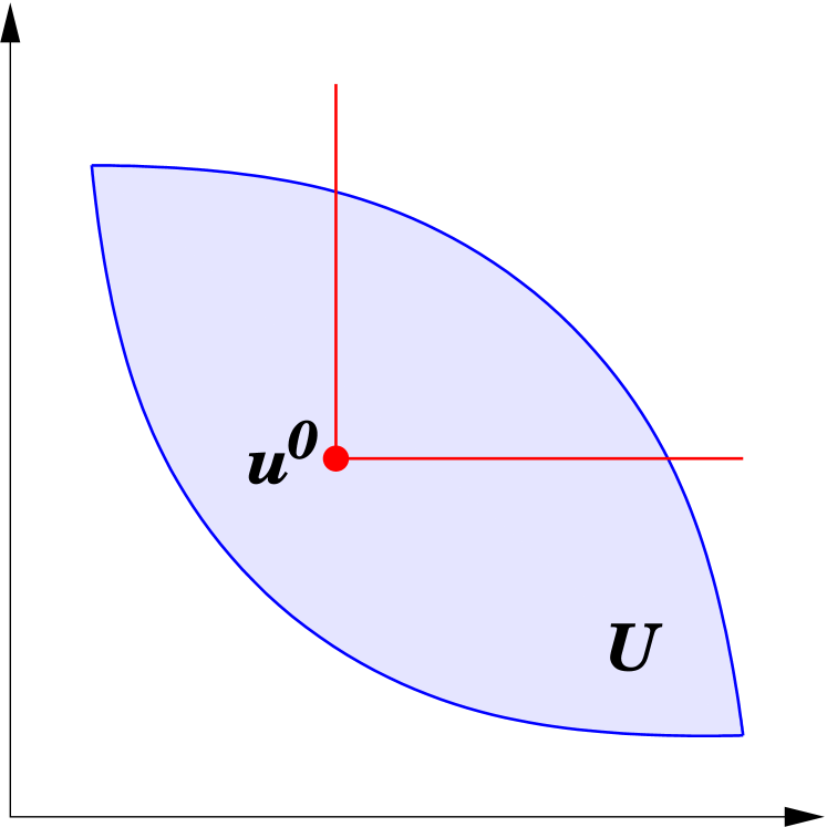
Figure 1: A Nash bargaining problem

The elements of $U$ are called outcomes and $\bou^{0}$ is the disagreement outcome. The interpretation of such a problem is as follows. A community of $K$ bargainers is faced with the problem to negotiate for a fair point in the convex set $U.$ If no agreement can be achieved by the bargainers, the disagreement utilities $u^{0}_{1},\dots,u^{0}_{K}$ will be the outcome of the game. Let $B_{K}$ denote the family of all $K$-person bargaining problems.
A bargaining solution is a function $F:B_{K}\to\mathbb{R}^{K}$ such that $F(U,\bou^{0})\in U$ for all $(U,\bou^{0})\in B_{K}.$ Nash suggested a solution that is based on four axioms, as given below.

(WPO) Weak Pareto optimality:
$F:B_{K}\to\mathbb{R}^{K}$ is called weakly Pareto optimal, if for all $(U,\bou^{0})\in B_{K}$ there exists no $\bou\in U$ satisfying $\bou>F(U,\bou^{0})$.

(SYM) Symmetry:
$F:B_{K}\to\mathbb{R}^{K}$ is symmetric if $F_{i}(U,\bou^{0})=F_{j}(U,\bou^{0})$ for all $(U,\bou^{0})\in B_{K}$ that are symmetric with respect to a subset $J\subseteq\{1,\dots,K\}$ for all $i,j\in J$ (i.e., $u_{i}^{0}=u_{j}^{0}$ and $(u_{1},u_{2},\dots,u_{i-1},u_{j},u_{i+1},\dots,u_{j-1},u_{i},u_{j+1},\dots\dots,u_{K})\in U$ for all $i<j\in J,\bou\in U$).

(SCI) Scale covariance:
$F:B_{K}\to\mathbb{R}^{K}$ is scale covariant if $F(\varphi(U),\varphi(\bou^{0}))=\varphi(F(U,\bou^{0}))$ for all $\varphi:\mathbb{R}^{K}\to\mathbb{R}^{K},\varphi(\bou)=\bar{\bou}$ with $\bar{u}_{i}=a_{i}u_{i}+b_{i}$, $a_{i},b_{i}\in\mathbb{R}$, $a_{i}>0,\ i=1,\dots,K$.

(IIA) Independence of irrelevant alternatives:
$F:B_{K}\to\mathbb{R}^{K}$ is independent of irrelevant alternatives, if $F(U,\bou^{0})=F(\bar{U},\bar{\bou}^{0})$ for all $(U,\bou^{0}),(\bar{U},\bar{\bou}^{0})\in B_{K}$ with $\bou^{0}=\bar{\bou}^{0},\ U\subseteq\bar{U}_{0}$ and $F(\bar{U},\bar{\bou}^{0})\in U$.

Remark. Weak Pareto optimality means that no bargainer can gain over the solution outcome. Symmetry, scale covariance and independence of irrelevant alternatives are the so called axioms of fairness. The symmetry property states that the solution does not depend on the specific label, i.e., users with both the same initial points and objectives will obtain the same performance. Scale covariance requires the solutions to be covariant under positive affine transformations. Independence of irrelevant alternatives demands that the solution outcome does not change when the set of possible outcomes shrinks but still contains the original solution.
These four axioms imply Pareto optimality which means that it is impossible to increase any player’s utility without decreasing another player’s utility.

The Nash bargaining solution is defined as follows.

Definition 4

A function $N:B_{K}\to\mathbb{R}^{K}$ is said to be a Nash bargaining solution (NBS) if

$$N(U,\bou^{0})=\operatorname{argmax}\Big{\{}\prod_{\begin{subarray}{c}1\leq j\leq K\\ u_{j}\neq u_{j}^{0}\end{subarray}}\left(u_{j}-u^{0}_{j}\right)\left|\bou\in U,\bou\geq\bou^{0}\right.\Big{\}},$$

whenever $U\backslash\{\bou^{0}\}\neq\varnothing$ and $N(U,\bou^{0})=\bou^{0},$ otherwise.

The NBS aims at maximizing the product of the users’ gain from cooperation, see Fig. 2 for the two dimensional case. In addition it is uniquely characterized by the four axioms stated above. The proof of the following theorem can be found in [19].

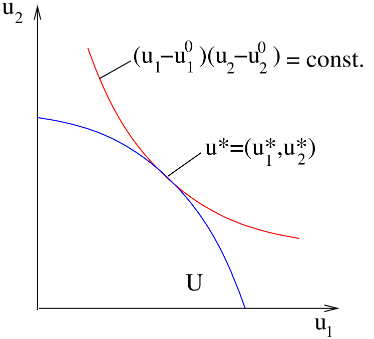
Figure 2: The Nash Bargaining Solution

Theorem 5

Let $F:B_{K}\to\mathbb{R}^{K}$ be a bargaining solution. Then the following two statements are equivalent:

1. $F=N.$

2. $F$ satisfies WPO, SYM, SCI, IIA.

In the following we consider the feasible power region

$${\cal P}={{\cal P}}_{\rm SIR}\cap{{\cal P}}_{\rm max}$$

with ${{\cal P}}_{\rm max}=\{\bop>{\bf 0}\mid p_{i}\leq p_{i,{\rm max}}\}$, as defined in (1) and (9).

Our aim is to single out one element of the power region ${\cal P}.$ There are many solution concepts to choose a reasonable element of ${\cal P},$ e.g. bargaining theory, proportional fairness, max-min fairness. We choose bargaining theory and the NBS in accordance with the above axioms.

Transmit power of each mobile station is bounded by $p_{i,{\rm max}}$. Due to limited battery power each user aims at using the lowest power possible. Hence we introduce a utility function $f_{i}$ for each mobile station $1\leq i\leq K$ as follows

$$f_{i}:{\cal P}\to\mathbb{R},\quad\bop\mapsto e^{p_{i,{\rm max}}}-e^{p_{i}}.$$

The task now is to find an element of the feasible power region such that the utility of each player is maximized. This task however is impossible to solve. As an alternative, we need to find an element in the utility set $f({\cal P})$ that is superior to other elements. The utility set is defined as the image of the utility functions

$$f({\cal P})=\{e^{\bop_{\rm max}}-e^{\bop}\mid\bop\in{\cal P}\},$$

where $e^{\bop}=(e^{p_{1}},\dots,e^{p_{K}})$ is defined componentwise and $e^{\bop_{\rm max}}=(e^{p_{1,{\rm max}}},\ldots,e^{p_{K,{\rm max}}})$ accordingly.

Clearly we should choose a Pareto optimal element. The question arises at which of the infinitely many Pareto optimal points the system should be operated. From the perspective of resource sharing, one of the natural criteria is the notion of fairness. This, in general is a loose term and there are many notions of fairness. One of the commonly used notions is that of max-min fairness which penalizes large users. Max-min fairness corresponds to a Pareto optimal point. However, it is not easy to take into account that users might have different requirements. A much more satisfactory approach is the use of fairness from game theory as introduced above. Another common solution concept of fairness is proportional fairness. It can be shown that proportional fairness leads in fact to the NBS. Therefor we confine ourselves to a game theoretic approach here.

In our cooperative game, players are formed by mobile stations, and they have to agree upon some element of the utility set $f({\cal P}).$ The bargaining set $U$ is now obtained by extending $f({\cal P})$ to

$$U=\left\{\bou\in\mathbb{R}^{K}\mid\exists\,\bop\in{\cal P}\text{ s.t.~{} }\bou\leq f(\bop)\right\}.$$ (12)

As is shown in [20] the convexity of $U$ follows since $f_{i}$ are concave functions. Fig. 3 generically depicts the utility set and its extension. Observe that the outcome of the cooperative game lies in $f({\cal P})$, so that the enlargement to $U$ is mainly of technical reasons to assure convexity.

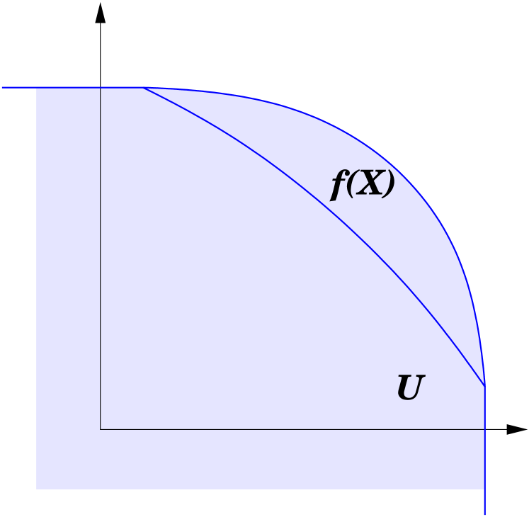
Figure 3: The extension $U$ of the utility set $f({\cal P})$

Moreover

$$\bou^{0}=-e^{\bop_{\rm max}}$$ (13)

represents the disagreement outcome, where each user has to transmit with its maximum power if the mobile stations fail to achieve an agreement. In summary, $(U,\bou^{0})$ is a K-person bargaining game. In the following the NBS of this game is determined. It turns out that the NBS coincides with the previously defined minimum power solution under function $h$ in (11). The proof follows easily from Definition 4.

Proposition 6

The unique NBS to the bargaining problem $(U,\bou^{0})$ defined in (12) and (13) is the solution to the following optimization problem:

$$\max\prod_{i=1}^{K}(e^{p_{i,{\rm max}}}-e^{p_{i}})$$ (14)

such that

$${\rm{SIR}}_{i}(\bop) \geq\gamma_{i},$$

$$p_{i} \geq 0,$$

$$p_{i,{\rm max}}-p_{i} \geq 0,\quad 1=1,\ldots,K.$$

Problem (14) is equivalent to minimizing function (11) subject to constraints (9). If the constraining set is nonempty, the solution is given by $\bop^{*}=\bopi(\bogamma)$ from (6), as is shown in Section III.

V Conclusion

This paper deals with the power control problem for a multiuser CDMA channel. It is shown that the power region is both convex and log-convex. It furthermore contains a uniformly minimal element $\bop^{*}$, at which any componentwise montone function attains its minimum. If there is no feasible power allocation we suggest the point of minimum distance to $\bop^{\ast}$ in the viable power region as a solution to the feasible minimum power problem. This point can be easily computed by a cyclic projection algorithm. The paper concludes with showing that for an appropriate utility function the minimum power problem with restricted power budget is obtained as the Nash bargaining solution for an adaptively defined cooperative game.

References

- [1] H. Boche and S. Stanczak, “Log-convexity of the minimum total power in CDMA systems with certain quality-of-services guaranteed,” To appear: IEEE Transactions on Information Theory, 2005.
- [2] L. Imhof and R. Mathar, “Capacity regions and optimal power allocation for CDMA cellular radio,” RWTH Aachen University, Institute of Theoretical Information Technology, Tech. Rep., June 2003.
- [3] ——, “The geometry of the capacity region for CDMA systems with general power constraints,” To appear: IEEE Transactions on Wireless Communications, 2005.
- [4] D. Tse and S. Hanly, “Linear multiuser receivers: effective interference, effective bandwidth and user capacity,” IEEE Transactions on Information Theory, vol. 45, no. 2, pp. 641–657, March 1999.
- [5] P. Viswanath, V. Anantharam, and D. Tse, “Optimal sequences, power control, and user capacity of synchronous CDMA systems with linear MMSE multiuser receivers,” IEEE Transactions on Information Theory, vol. 45, no. 6, pp. 1968–1983, September 1999.
- [6] D. Catrein, L. Imhof, and R. Mathar, “Power control, capacity, and duality of up- and downlink in cellular CDMA radio,” IEEE Transactions on Communications, vol. 52, no. 10, pp. 1777–1785, October 2004.
- [7] S. Hanly, “An algorithm for combined cell-site selection and power control to maximize cellular spread spectrum capacity,” IEEE Journal on Selected Areas in Communications, vol. 13, no. 7, pp. 1332–1340, September 1995.
- [8] L. Mendo and J. Hernando, “On dimension reduction for the power control problem,” IEEE Transactions on Communications, vol. 49, no. 2, pp. 243–248, February 2001.
- [9] R. Yates, “A framework for uplink power control in cellular radio systems,” IEEE Journal on Selected Areas in Communications, vol. 13, no. 7, pp. 1341–1348, September 1995.
- [10] S. Kandukuri and S. Boyd, “Optimal power control in interference-limited fading wireless channels with outage-probability specifications,” IEEE Transactions on Wireless Communications, vol. 1, no. 1, pp. 46–55, January 2002.
- [11] J. Papandriopoulos, J. Evans, and S. Dey, “Outage-based optimal power control for generalized multiuser fading systems,” To appear: IEEE Transactions on Communications, 2005.
- [12] ——, “Optimal power control for Rayleigh-faded multiuser systems with outage constraints,” To appear: IEEE Transactions on Wireless Communications, 2005.
- [13] S. Ulukus and R. Yates, “Stochastic power control for cellular radio systems,” IEEE Transactions on Communications, vol. 46, no. 6, pp. 784–798, June 1998.
- [14] M. Varanasi and D. Das, “Fast stochastic power control algorithms for nonlinear multiuser receivers,” IEEE Transactions on Communications, vol. 50, no. 11, pp. 1817–1827, November 2002.
- [15] A. Roberts and D. Varberg, Convex Functions. New York: Academic Press, 1973.
- [16] D. Luenberger, Optimization by Vector Space Methods. New York: Wiley, 1969.
- [17] N. Gaffke and R. Mathar, “A cyclic projection algorithm via duality,” Metrika, vol. 36, pp. 29–54, 1989.
- [18] A. Muthoo, Bargaining Theory with Application. Cambridge: Cambridge University Press, 1999.
- [19] A. Stefanescu and M. Stefanescu, “The arbitrated solution for multi-objective convex programming,” Rev. Roumaine Math. Pures Appl., vol. 29, pp. 593–598, 1984.
- [20] A. Feiten and R. Mathar, “A game theoretic approach to capacity sharing in CDMA radio networks,” in Proceedings Australian Telecommunications and Applications Conference, ATNAC04, Sydney, 2004.