Computing over the Reals: Foundations for Scientific Computing

Abstract

We give a detailed treatment of the “bit-model” of computability and complexity of real functions and subsets of ${{\mathbb{R}}}^{n}$, and argue that this is a good way to formalize many problems of scientific computation. In Section 1 we also discuss the alternative Blum-Shub-Smale model. In the final section we discuss the issue of whether physical systems could defeat the Church-Turing Thesis.

1 Introduction

The problems of scientific computing often arise from the study of continuous processes, and questions of computability and complexity over the reals are of central importance in laying the foundations for the subject. The first step is defining a suitable computational model for functions over the reals.

Computability and complexity over discrete spaces have been very well studied since the 1930s. Different approaches have been proved to yield equivalent definitions of computability and nearly equivalent definitions of complexity. From the tradition of formal logic we have the notions of recursiveness and Turing machine, and from computational complexity we have variations on Turing machines and abstract Random Access Machines (RAMs), which closely model actual computers. All of these converge to define the same well-accepted notion of computability. The Church-Turing thesis asserts that this formal notion of computability is broad enough, at least in the discrete setting, to include all functions that could reasonably construed to be computable.

In the continuous setting, where the objects are numbers in ${{\mathbb{R}}}$, computability and complexity have received less attention and there is no one accepted computation model. Alan Turing defined the notion of a single computable real number in his landmark 1936 paper [Tur36]: a real number is computable if its decimal expansion can be computed in the discrete sense (i.e. output by some Turing machine). But he did not go on to define the notion of computable real function.

There are now two main approaches to modeling computation with real number inputs. The first approach, which we call the bit-model and which is the subject of this paper, reflects the fact that computers can only store finite approximations to real numbers. Roughly speaking, a real function $f$ is computable in the bit model if there is an algorithm which, given a good rational approximation to $x$, finds a good rational approximation to $f(x)$.

The second approach is the algebraic approach, which abstracts away the messiness of finite approximations and assumes that real numbers can be represented exactly and each arithmetic operation can be performed exactly in one step. The complexity of a computation is usually taken to be the number of arithmetic operations (for example additions and multiplications) performed. The algebraic approach applies naturally to arbitrary rings and fields, although for modeling scientific computation the underlying structure is usually ${{\mathbb{R}}}$ or ${{\mathbb{C}}}$. Algebraic complexity theory goes back to the 1950s (see [BM75, BCS97] for surveys).

For scientific computing the most influential model in the algebraic setting is due to Blum, Shub and Smale (BSS) [BSS89]. The model and its theory are thoroughly developed in the book [BCSS98] (see also the article [Blum04] in the AMS Notices for an exposition). In the BSS model, the computer has registers which can hold arbitrary elements of the underlying ring $R$ and performs exact arithmetic ($+,-,\cdot$, and $\div$ in the case $R$ is a field) and computer programs can branch on conditions based on exact comparisons between ring elements ($=$, and also $<$, in the case of an ordered field). Newton’s method, for example, can be nicely presented in the BSS model as a program (which may not halt) for finding an approximate zero of a rational function, when $R={{\mathbb{R}}}$. A nice feature of the BSS model is its generality: the underlying ring $R$ is arbitrary, and the resulting computability theory can be studied for each $R$. In particular, when $R={{\mathbb{Z}}}_{2}$, the model is equivalent to the standard bit computer model in the discrete setting.

One of the big successes of discrete computability theory is is the uncomputability results; especially the solution of Hilbert’s 10th problem [Mat93]. The theorem states that there is no procedure (e.g. no Turing machine) which always correctly determines whether a given Diophantine equation has a solution. The result is convincing because of general acceptance of the Church-Turing thesis.

A weakness of the BSS approach as a model of scientific computing is that uncomputability results do not correspond to computing practice in the case $R={{\mathbb{R}}}$. Since intermediate register values of a computation are rational functions of the inputs, it is not hard to see that simple transcendental functions such as $e^{x}$ are not explicitly computable by a BSS machine. In the bit model these functions are computable because the underlying philosophy is that the inputs and outputs to the computer are rational approximations to the actual real numbers they represent. The definition of computability in the BSS model might be modified to allow the program to approximate the exact output values, so that functions like $e^{x}$ become computable. However formulating a good general definition in the BSS model along these lines is not straightforward: see [Sma97] for an informal treatment and [Brv05] for a discussion and a possible formal model.

For uncomputability results, BSS theory concentrates on set decidability rather than function computation. A set $C\subseteq{{\mathbb{R}}}^{n}$ is decidable if some BSS computer program halts on each input $\vec{x}\in{{\mathbb{R}}}^{n}$ and outputs either 1 or 0, depending on whether $\vec{x}\in C$. Theorem 1 in [BCSS98] states that if $C\subseteq{{\mathbb{R}}}^{n}$ is decided by a BSS program over ${{\mathbb{R}}}$ then $C$ is a countable disjoint union of semi-algebraic sets. A number of sets are proved undecidable as corollaries, including the Mandelbrot set and all nondegenerate Julia sets (Fig. 2). However again it is hard to interpret these undecidability results in terms of practical computing, because simple subsets of ${{\mathbb{R}}}^{2}$ which can be easily “drawn”, such as the Koch snowflake and the graph of $y=e^{x}$ (Fig. 1) are undecidable in this sense [Brt03].

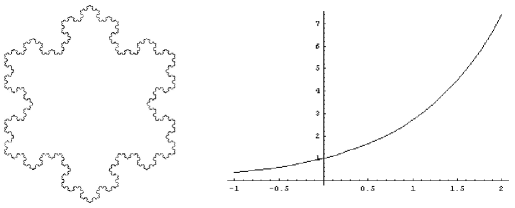
Figure 1: The Koch snowflake and the graph of the equation $y=e^{x}$

In the bit model there is a nice definition of decidability (bit-computability) for bounded subsets of ${{\mathbb{R}}}^{n}$ (Section 3.3). For the case of ${{\mathbb{R}}}^{2}$, the idea is that the set is bit-computable if some computer program can draw it on a computer screen. The program should be able to zoom in at any point in the set and draw a neighborhood of that point with arbitrarily fine detail. Such programs can be easily written for simple sets such as the Koch snowflake and the graph of the equation $y=e^{x}$, and more sophisticated programs can be written for many Julia sets (Section 4). A Google search on the World Wide Web turns up programs that apparently do the same for the Mandelbrot set. However no one knows how accurate these programs are. The bit computability of the Mandelbrot set is an open question, although it holds subject to a major conjecture (Section 4). Because of the Church-Turing thesis, a proof of bit-uncomputability of the Mandelbrot set would carry some force: the programs purporting to draw it must draw it wrong, at least at some level of detail.

In the rest of the paper we concentrate on the bit model, because we believe that this is the most accurate abstraction of how computers are used to solve problems over the reals. The bit model is not widely appreciated in the mathematical community, perhaps because its principal references are not written to appeal to numerical analysts. In contrast the BSS model has received widespread attention, partly because its presentation [BSS89], and especially the excellent reference [BCSS98], not only present the model but provide a rigorous treatment of matters of interest in scientific computation. The authors deserve credit not just for presenting an elegant model, but also for arousing interest in foundational issues for numerical analysis, and inspiring considerable research. Undoubtedly the concept of abstracting away round-off error in computations over the reals poses important natural questions. One example is linear programming: Although polynomial time algorithms are known for solving linear programming problems in the bit model, no such algorithm is known for the BSS model. The commonly-used simplex algorithm can be neatly formalized in the BSS model, but it requires exponential time in the worst case. It would be very nice to find a polynomial time BSS algorithm for linear programming.

Here is an outline of the remaining sections. Section 2 gives examples of easy and hard computational problems over the reals. Section 3 motivates and defines the bit model both for computing real functions and subsets of ${{\mathbb{R}}}^{n}$. Computational complexity issues are discussed. Section 4 treats the computability and complexity of the Mandelbrot and Julia sets. Simple programs are available which seem to compute the Mandelbrot set, but they may draw pieces which should not be there. The bit-computability of the Mandelbrot set is open, but it is implied by a major conjecture. Many Julia sets are not only computable, but are efficiently computable (in polynomial time). On the other hand some Julia sets are uncomputable in a fundamental sense. Finally Section 5 discusses a fundamental question related to the Church-Turing thesis: are there physical systems that can compute functions which are uncomputable in the standard computer model?

Some of the material presented here is given in more detail in [Brv05]. See [Ko91] and [Wei00] for general references on bit-computability models.

Acknowledgments The authors are grateful to the following people for helpful comments on a preliminary version of this paper: Eric Allender, Lenore Blum, Peter Hertling, Ken Jackson, Charles Rackoff, Klaus Weihrauch, and Michael Yampolsky.

2 Examples of “easy” and “hard” problems

2.1 “Easy” problems

We start with examples of problems over the reals that should be “easy” according to any reasonable model. The everyday operations, such as addition, subtraction and multiplication should be considered easy. More generally, any of the operations that can be found on a common calculator can be regarded as “easy”, at least in some reasonable region. Such functions include, among others, $\sin x$, $e^{x}$, $\sqrt{x}$, and $\log x$.

Functions with singularities, such as $x\div y$ and $\tan x$ are easily computable on any closed region which excludes the singularities. The computational problem usually gets harder as we approach the singularity point. For example, computing $\tan x$ becomes increasingly difficult as $x$ tends to $\frac{\pi}{2}$, because the expression becomes increasingly sensitive in $x$.

Some basic numerical problems that are known to have efficient solutions should also be relatively “easy” in the model. This includes inverting a well conditioned matrix $A$. A matrix is well conditioned in this setting if $A^{-1}$ does not vary too sharply under small perturbations of $A$.

Simple problems that arise naturally in the discrete setting should usually remain simple in the continuous setting. This includes problems such as sorting a list of real numbers and finding shortest paths in a graph with real edge lengths.

When one considers subsets of ${{\mathbb{R}}}^{2}$, a set should be considered “easy”, if we can draw it quickly with an arbitrarily high precision. Examples include simple “paintbrush” shapes, such as the ball $B((0,0),2)$ in ${{\mathbb{R}}}^{2}$, as well as simple fractal sets, such as the Koch snowflake (Fig. 1).

To summarize, the model should classify a problem as “easy”, if there is an efficient algorithm to solve it in some practical sense. This algorithm may be inspired by a discrete algorithm, a numerical-analytic technique, or both.

2.2 “Hard” problems

Naturally, the “hard” problems are the ones for which no efficient algorithm exists. For example, it is hard to compute an inverse $A^{-1}$ of a poorly conditioned matrix $A$. Note that even simple numerical problems, such as division $(x+1)\div(y-1)$, become increasingly difficult in the poorly conditioned case. It becomes increasingly hard to evaluate the latter expression as $y$ approaches $1$.

Many problems that appear to be computationally hard arise while trying to model processes in nature. A famous example is the $N$-body problem, which simulates the motion of planets. An even harder example is solving the Navier-Stokes equations used in simulations for fluid mechanics. We will return to questions of hardness in physical systems in Section 5.

Another class of problems that should be hard is natural extensions of very difficult discrete problems. Consider, for example, the subset sum problem. In this problem we are given a list $S=\{a_{1},a_{2},\ldots,a_{n}\}$ of numbers and a number $A$. Our goal is to decide whether there is a subset $\{a_{i_{1}},a_{i_{2}},\ldots,a_{i_{k}}\}$ that adds up to $A$, i.e. $a_{i_{1}}+a_{i_{2}}+\ldots+a_{i_{k}}=A$. This problem is widely believed not to have an efficient solution in the discrete case. In fact it is $NP$-complete in this case ([GJ79]), and having a polynomial time algorithm for it would imply that $P=NP$, which is believed to be unlikely. There is no reason to think that it should be any easier in the continuous setting than in the discrete case.

The hardness of numerical problems may significantly vary with the domain of application. Consider for example the problem of computing the integral $I(x)=\int_{0}^{x}f(t)dt$. While it is very easy to compute $I(x)$ from $f(x)$ in the case $f$ is a polynomial, it can be extremely difficult in the case $f$ is a more general efficiently computable function.

2.3 Quasi-fractal examples: the Mandelbrot and Julia sets

The Mandelbrot and the Julia sets are common examples of computer-drawn sets. Beautiful high-resolution images have become available to us with the rapid development of computers. Amazingly, these extremely complex images arise from very simple discrete iterated processes on the complex plane ${{\mathbb{C}}}$.

For a point $c\in{{\mathbb{C}}}$, define $f_{c}(z)=z^{2}+c$. $c$ is said to be in the Mandelbrot set $M$ if the iterated sequence $c,f_{c}(c),f_{c}(f_{c}(c)),\ldots$ does not diverge to $\infty$. While (we believe) very precise images of $M$ can be generated on a computer, proving that these images approximate $M$ would probably involve solving some difficult open questions about it.

The family of Julia sets is parameterized by functions. In the simple case of quadratic functions $f_{c}(z)=z^{2}+c$, the filled Julia set $K_{c}$ is the set of points $x$, such that the sequence $x,f_{c}(x),f_{c}(f_{c}(x)),\ldots$ does not diverge to $\infty$. The Julia set $J_{c}$ is defined as the boundary of $K_{c}$. While many Julia sets, such as the ones in Fig. 2, are quite easy to draw, there are explicit sets of which we simply cannot produce useful pictures.

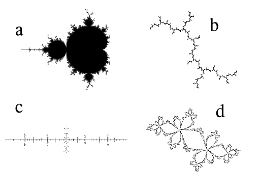
Figure 2: a: the Mandelbrot set; b-d: Julia sets with parameter values of $i$, $-1.57$ and $0.5+0.56i$, respectively.

As we see, it is not a priori clear whether these sets should be “easy” or “hard”. This gives rise to a series of questions:

• Is the Mandelbrot set computable?

• Which Julia sets are computable?

• Can the Mandelbrot sets and its zoom-ins be drawn quickly on a computer?

• Which Julia sets and their zoom-ins can be drawn quickly on a computer?

These questions are meaningless unless we agree upon a model of computation for this setting. In the following sections we develop such a model, based on “drawability” on a computer.

3 The bit model

3.1 Bit computability for functions

The motivation behind the bit model of computation is idealizing the process of scientific computing. Consider for example the simple task of computing the function $x\mapsto e^{x}$ for an $x$ in the interval $[-1,1]$. The most natural solution appears to be by taking the Taylor series expansion around $0$:

$$e^{x}=\sum_{k=0}^{\infty}\frac{x^{k}}{k!}.$$ (1)

Obviously in a practical computation we will only be able to add up a finite number of terms from (1). How many terms should we consider? By taking more terms, we can improve the precision of the computation. On the other hand, we pay the price of increasing the running time as we consider more terms. The answer is that we should take just enough terms to satisfy our precision needs.

Depending on the application, we might need the value of $e^{x}$ within different degrees of precision. Suppose we are trying to compute it with a precision of $2^{-n}$. That is, on an input $x$ we need to output a $y$ such that $|e^{x}-y|<2^{-n}$. It suffices to take $n+1$ terms from (1) to achieve this level of approximation. Indeed, assuming $n\geq 4$, for any $x\in[-1,1]$,

$$\left|e^{x}-\sum_{k=0}^{n}\frac{x^{k}}{k!}\right|=\left|\sum_{k={n+1}}^{\infty}\frac{x^{k}}{k!}\right|\leq\sum_{k={n+1}}^{\infty}\frac{|x^{k}|}{k!}\leq\sum_{k={n+1}}^{\infty}\frac{1}{k!}<\sum_{k={n+1}}^{\infty}\frac{1}{2^{k+1}}=2^{-(n+1)}.$$

In fact, a smaller number of terms suffices to achieve the desired precision. We take a portion of the series that yields error $2^{-(n+1)}<2^{-n}$, to allow room for computation (round-off) errors in the evaluation of the finite sum. All we have to do now is to evaluate the polynomial $p_{n}(x)=\sum_{k=0}^{n}\frac{x^{k}}{k!}$ within an error of $2^{-(n+1)}$. To do this, we need to know $x$ with a certain precision $2^{-m}$. It is convenient to use dyadic rationals to express approximations to $x$ and $e^{x}$, where the dyadic rationals form the set

$${{\mathbb{D}}}=\{\mbox{$\frac{m}{2^{n}}$}\mid m\in{{\mathbb{Z}}},n\in{{\mathbb{N}}}\}.$$

We can then take a dyadic $q=\frac{r}{2^{s}}\in{{\mathbb{D}}}$ such that $|x-q|<2^{-m}$, and evaluate $p_{n}(q)$ within an error of $2^{-(n+2)}$ using finite precision dyadic arithmetic. This gives us an approximation $y\in{{\mathbb{D}}}$ of $p_{n}(q)$ such that $|y-p_{n}(q)|<2^{-(n+2)}$. In our example, an assumption $|x-q|<2^{-(n+4)}$ guarantees that $|p_{n}(x)-p_{n}(q)|<2^{-(n+2)}$, and we can take $m=n+4$. To summarize, we have

$$|e^{x}-y|\leq|e^{x}-p_{n}(x)|+|p_{n}(x)-p_{n}(q)|+|p_{n}(q)-y|<2^{-(n+1)}+2^{-(n+2)}+2^{-(n+2)}=2^{-n},$$

and $y$ is the answer we want. The running time of the computation is dominated by the time it takes to compute our approximation to $p_{n}(q)$. Note that this entire computation is done over the dyadic rationals, and can be implemented on a computer.

To find the answer we only needed to know $x$ within an error of $2^{-(n+4)}$. This is especially important when one tries to compose several computations. For example, to compute $e^{e^{x}-1}$ within en error $2^{-n}$ on the appropriate interval, one would need to know $x$ within an error of $2^{-(n+8)}$.

While evaluating the function $e^{x}$ is hardly a challenge for scientific computing, the process described above illustrates the main ideas in the bit model of computation. Below are the main points that we have seen in this example, and that characterize the bit model for computing functions. Suppose we are trying to compute $f:[a,b]\rightarrow{{\mathbb{R}}}^{n}$. Denote the program computing $f$ by $M_{f}$.

• The goal of $M_{f}(x,n)$ is to compute $f(x)$ within the error of $2^{-n}$;

• $M_{f}$ computes a precision parameter $m$, it needs to know $x$ within an error of $2^{-m}$ to proceed with the computation;

• $M_{f}$ receives a dyadic $q=\frac{r}{2^{s}}$ such that $|x-q|<2^{-m}$;

• $M_{f}$ computes a dyadic $y$ such that $|f(x)-y|<2^{-n}$;

• the running time of $M_{f}(x,n)$ is the time it takes to compute $m$ plus the time it takes to compute $y$ from $q$ (both of which have finite representations by bits).

Note that the entire computation of $M_{f}$ is performed only with finitely presented dyadic numbers. There is a nice way to present the computation using oracle terminology. An oracle for a real number $x$ is a function $\phi:{{\mathbb{N}}}\rightarrow{{\mathbb{D}}}$ such that for all $n$, $|\phi(n)-x|<2^{-n}$. Note that the $q$ in the description above can be taken to be $q=\phi(m)$. Instead of querying the value of $x$ once, we can allow $M_{f}$ an unlimited access to the oracle $\phi$. The only limitation would be that the time it takes $M_{f}$ to read the output of $\phi(m)$ is at least $m$. We emphasize the fact that $x$ is presented to $M_{f}$ as an oracle by writing $M_{f}^{\phi}(n)$ instead of $M_{f}(x,n)$. Just as the quality of the answer of $M_{f}(x,n)$ should not depend on the specific $2^{-m}$-approximation $q$ for $x$, $M_{f}^{\phi}(n)$ should output a $2^{-n}$-approximation of $f(x)$ for any valid oracle $\phi$ for $x$.

The running time $T(n)$ of $M_{f}^{\phi}(n)$ is the worst case time a computation on this machine can take with a valid input and precision $n$. If $T(n)$ is bounded by some polynomial $p(n)$, we say that $M_{f}^{\phi}$ works in polynomial time.

The output of $M_{f}^{\phi}(n)$ can be viewed itself as an oracle for $f(x)$. This allows us to compose functions. For example, given a machine $M_{f}^{\phi}(n)$ for computing $f(x)$, and a machine $M_{g}^{\phi}(n)$ for computing $g(x)$, we can compute $f\circ g(x)$ by $M_{f}^{M_{g}^{\phi}}(n)$.

This is the bit-computability notion for functions. It was first proposed by Grzegorczyk [Grz55] and Lacombe [Lac55]. It has been since developed and generalized. More recent references on the subject include [Ko91], [PR89], and [Wei00]. Let us see some examples to illustrate this notion.

3.2 Examples of bit-computability

We start with a family of the simplest possible functions, the constant functions. For a function $f(x)=a$, $a\in{{\mathbb{R}}}$ a constant, we can completely ignore the input $x$. The complexity of computing $f(x)$ with precision $2^{-n}$ is the complexity of computing the number $a$ within this error. In the original work by Turing [Tur36], the motivation for introducing Turing machines was defining which numbers can be computed, and which cannot.

For example, the numbers $\frac{1}{3}=(0.01010101\ldots)_{2}$ and $\sqrt{2}$ appear to be “easy”, with the latter being “harder” than the former. There are also easy algorithms for computing transcendental numbers such as $\pi$ and $e$. But there are only countably many programs, hence all but countably many reals cannot be approximated by any of them. To give a specific example of a very hard number, consider some standard encoding of all the Diophantine equations, $\phi:\{equations\}\rightarrow{{\mathbb{N}}}$. Let $D=\{\phi(EQ)~{}:~{}\mbox{$EQ$ is a solvable equation}\}\subset{{\mathbb{N}}}$, and

$$d=\sum_{n\in D}4^{-n}.$$

Then computing $d$ with an arbitrarily high precision would allow us to decide whether $\phi(EQ)$ is in $D$ for any specific Diophantine equation $EQ$. This would contradict the solution to Hilbert’s 10th Problem, which states that no such decision procedure can exist (see [Mat93], for example).

The following example will illustrate the bit-computability of a more general function.

Example: Consider the function $f(x)=\sqrt[3]{1-x^{3}}$ on the interval $[0,1]$. It is a composition of two functions: $g:x\mapsto 1-x^{3}$ and $h:x\mapsto\sqrt[3]{x}$, both on the $[0,1]$ interval. $g$ is easier to compute in this case. To obtain $g(x)$ with precision $2^{-n}$ it suffices to query for an approximation $q\in[0,1]$ of $x$ with precision $2^{-(n+2)}$, and to return $a=1-q^{3}$, computed within an error of $2^{-(n+2)}$. Note that the second operation is done entirely with bits. We obtain an answer $a$ such that

$$|a-g(x)|\leq|a-g(q)|+|q^{3}-x^{3}|<2^{-(n+2)}+|q-x|\cdot|q^{2}+qx+x^{2}|\leq 2^{-(n+2)}+2^{-(n+2)}\cdot 3=2^{-n}.$$

The function $h(x)$ is slightly trickier to compute. One possible approach is to use Newton’s method to solve (approximately) the equation $\lambda^{3}-x=0$ to obtain $\lambda=\sqrt[3]{x}$. The fact that $g(x)$ and $h(x)$ are computable is not surprising. In fact, both these functions can be found on a common scientific calculator.

In general, all “calculator functions” are computable on a properly chosen domain. For example, $x\mapsto 1/x$ is computable on any domain which excludes $0$. We can bound the time required to compute the inverse, if the domain is properly bounded away from $0$. The only true limiting factor here is that computable functions as described above must be continuous on the domain of their application. This is because the value of $f(x)$ we compute must be a good approximation for all points near $x$.

Theorem 1

Suppose that a function $f:S\rightarrow{{\mathbb{R}}}^{k}$ is computable. Then $f$ must be continuous.

This puts a limitation on the applicability on the computability notion above. While it is “good” at classifying continuous functions, it classifies all discontinuous functions, however simple, as being uncomputable. We will return to this point later in Section 3.5.

3.3 Bit-computability for sets

Just as the bit-computability of functions formalizes finite-precision numerical computation, we would like the bit-computability of sets to formalize the process of generating images of subsets in ${{\mathbb{R}}}^{k}$, such as the Mandelbrot and Julia sets discussed in Section 2.3.

An image is a collection of pixels, which can be taken to be small balls or cubes of size $\varepsilon$. $\varepsilon$ can be seen as the resolution of the image. The smaller it is, the finer the image is. The hardness of producing the image generally increases as $\varepsilon$ gets smaller. A collection of pixels $P$ is a good image of a bounded set $S$ if the following conditions are fulfilled:

• $P$ covers $S$. This ensures that we “see” the entire set $P$, and

• $P$ is contained in the $\varepsilon$-neighborhood of $S$. This ensures that we don’t get “irrelevant” components which are far from $S$.

It is convenient to take $\varepsilon=4\cdot 2^{-n}$ – our computation precision in this case.

Suppose now that we are trying to construct $P$ as a union of pixels of radius $2^{-n}$ centered at grid points $(2^{-(n+k)}\cdot{{\mathbb{Z}}})^{k}$. The basic decision we have to make is whether to draw each particular pixel or not, so that the union $P$ would satisfy the conditions above. To ensure that $P$ covers $S$, we include all the pixels that intersect with $S$. To satisfy the second condition, we exclude all the pixels that are $2^{-n}$-far from $S$. If none of these conditions holds, we are in the “gray” area, and either including or excluding a pixel is fine. In other words, we should compute a function from the family

$$f(d,n)=\left\{\begin{array}[]{ll}1&\mbox{ if }B(d,2^{-n})\cap S\neq\emptyset\\ 0&\mbox{ if }B(d,2\cdot 2^{-n})\cap S=\emptyset\\ 0\mbox{ or }1&\mbox{ otherwise }\end{array}\right.$$ (2)

for every point $d\in(2^{-(n+k)}\cdot{{\mathbb{Z}}})^{k}$. Here $f$ is computed in the classical discrete sense.

Example: A “simple” set, such as a point, line segment, circle, ellipse, etc. is computable if and only if all of its parameters are computable numbers. For example, a circle is computable if and only if the coordinates of its center and its radius are computable.

The way we have arrived at the definition of bit-computability might suggest that it is specifically tailored to computer-graphics needs and is not mathematically robust. This is not the case, as will be seen in the following theorem. Recall that the Hausdorff distance between bounded subsets of ${{\mathbb{R}}}^{k}$ is defined as

$$d_{H}(S,T)=\inf\{d~{}:~{}S\subset B(T,d),\mbox{ and }T\subset B(S,d)\}.$$

We have the following.

Theorem 2

Let $S\subset{{\mathbb{R}}}^{k}$ be a bounded set. Then the following are equivalent.

1. A function from the family (2) is computable.

2. There is a program that for any $\varepsilon>0$ gives an $\varepsilon$-approximation of $S$ in the Hausdorff metric.

3. The distance function $d_{S}(x)=\inf\{|x-y|:y\in$S$\}$ is bit-computable.

1. and 3. remain equivalent even if $S$ is not bounded.

Example: The finite approximations $K_{i}$ of the Koch snowflake are polygons that are obviously computable. The convergence $K_{i}\rightarrow K$ is uniform in the Hausdorff metric. So $K$ can be approximated in the Hausdorff metric with any desired precision. Thus the Koch snowflake is bit-computable.

The last characterization of set bit-computability in Theorem 2 connects the computability of sets and functions. There is another natural connection between the computability notions for these objects – through plots of a function’s graph.

Theorem 3

Let $D\subset{{\mathbb{R}}}^{k}$ be a closed and bounded computable domain, and let $f:D\rightarrow{{\mathbb{R}}}$ be a continuous function. Then $f$ is computable as a function if and only if the graph $\Gamma_{f}=\{(x,f(x)):x\in D\}$ is computable as a set.

Example: Consider the set $S=\{(x,y):x,y\in[0,1],~{}x^{3}+y^{3}=1\}$. It is the graph of the function $f(x)=\sqrt[3]{1-x^{3}}$ on $[0,1]$, which has been seen to be computable in Section 3.2. By Theorem 3, $S$ is a bit-computable set. This is despite the fact (pointed out in [Blum04]) that the only rational points in $S$ are $(0,1)$ and $(1,0)$.

The bit computability notion dates back to Lacombe [Lac58]. We refer the reader to [BW99, Wei00, Brv05] for a more detailed discussion.

3.4 Computational complexity in the bit model

Since the basic object in the discussion above is a Turing Machine, the computational complexity for the bit model follows naturally from the standard notions of computational complexity in the discrete setting. Basically, the time cost of a computation is the number of bit operations required.

For example, the time complexity $T_{\pi}(n)$ for computing the number $\pi$ is the number of bit operations required to compute the first $n$ binary digits of a $2^{-n}$-approximation of $\pi$. The time complexity $T_{e^{x}}(n)$ of computing the exponential function $x\mapsto e^{x}$ on $[-1,1]$, is the number of bit operations it takes to compute a $2^{-n}$-approximation of $e^{x}$ given an $x\in[-1,1]$. This running time is assessed at the worst possible admissible $x$. We have seen that both $T_{\pi}(n)$ and $T_{e^{x}}(n)$ are bounded by a polynomial in $n$.

This computational complexity notion can be used to assess the hardness of the different numerical-analytic problems arising in scientific computing. For example, the dependence of matrix inversion hardness on the condition number of the matrix fits nicely into this setting.

Schönhage [Sch82, Sch87] has shown how the fundamental theorem of algebra can be implemented by a polynomial time algorithm in the bit model. More precisely, he has shown how to solve the following problem in time $O((n^{3}+n^{2}s)\log^{3}(ns))$: Given any polynomial $P(z)=a_{n}z^{n}+\ldots+a_{0}$ with $a_{j}\in{{\mathbb{C}}}$ and $|P|=\sum_{v}|a_{v}|\leq 1$, and given any $s\in{{\mathbb{N}}}$, find approximate linear factors $L_{j}(z)=u_{j}z+v_{j}$ $(1\leq j\leq n)$ such that $|P-L_{1}L_{2}\cdots L_{n}|<2^{-s}$ holds.

The complexity of computing a set is the time $T(n)$ it takes to decide one pixel. More formally, it is the time required to compute a function from the family (2). Thus a set is polynomial-time computable if it takes time polynomial in $n$ to decide one pixel of resolution $2^{-n}$.

To see why this is the “right” definition, suppose we are trying to draw a set $S$ on a computer screen which has a $1000\times 1000$ pixel resolution. A $2^{-n}$-zoomed in picture of $S$ has $O(2^{2n})$ pixels of size $2^{-n}$, and it would take time $O(T(n)\cdot 2^{2n})$ to compute. This quantity is exponential in $n$, even if $T(n)$ is bounded by a polynomial. But we are drawing $S$ on a finite-resolution display, and we will only need to draw $1000\cdot 1000=10^{6}$ pixels. Hence the running time would be $O(10^{6}\cdot T(n))=O(T(n))$. This running is polynomial in $n$ if and only if $T(n)$ is polynomial. Hence $T(n)$ reflects the ‘true’ cost of zooming in, when drawing $S$.

3.5 Beyond the continuous case

As we have seen earlier, the bit model notion of computability is very intuitive for sets and for continuous functions. However, by Theorem 1 it completely excludes even the simplest discontinuous functions. Consider for example the step function

$$s_{0}(x)=\left\{\begin{array}[]{ll}0,&\mbox{if }x<0\\ 1,&\mbox{if }x\geq 0\end{array}\right.$$ (3)

The function is bit computable on any domain which excludes $0$. One could make the argument that a physical device really cannot compute $s_{0}$. There is no bound on the precision of $x$ needed to compute $s_{0}(x)$ near $0$. Hence no finite approximation of $x$ suffices to compute $s_{0}$ even within an error of $1/3$.

On the other hand, one might want to include this function, and other simple functions in the computable class, because the primary goal of this classification is to distinguish between “easy” and “hard” problems, and computing $s_{0}$ does not look hard. One possibility is to say that a function is computable if we can plot its graph. By Theorem 3, this definition extends the standard bit-computability definition in the continuous case. It is obvious that is makes $s_{0}$ computable, since the graph of $s_{0}$ is just a union of two rays. The notion of computational complexity can be extended into this more general setting as well. More details can be found in [Brv05].

4 How hard are the Mandelbrot and Julia sets?

First let us consider questions of computability of the Mandelbrot set $M$ (which was defined in Section 2.3). Despite the relatively simple process defining $M$, the set itself is extremely complex, and exhibits different kinds of behaviors as we zoom into it. In Fig. 3 we see some of the variety of images arising in $M$.

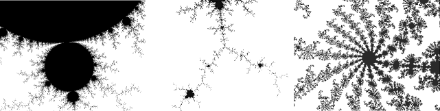
Figure 3: A variety of different images arising in zoom-ins of the Mandelbrot set

The most common algorithm used to compute $M$ is presented on Fig. 4. The idea is to fix some number $T$, which is the number of steps for which we are willing to iterate. Then for every gridpoint $c$ iterate $f_{c}(z)=z^{2}+c$ on $c$ for at most $T$ steps. If the orbit escapes $B(0,2)$, we know that $c\notin M$. Otherwise, we say that $c\in M$. This is equivalent to taking the inverse image of $B(0,2)$ under the polynomial map $f^{T}(c)=\underbrace{f_{c}\circ f_{c}\circ\ldots\circ f_{c}}_{T\mbox{ times}}(c)$. In Fig. 4 (right) a few of these inverse images and their convergence to $M$ are shown.

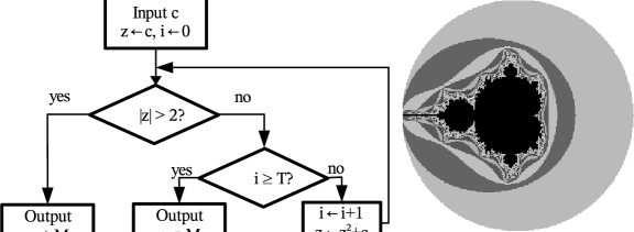
Figure 4: The naïve algorithm for computing $M$, and some of its outputs

One problem with this algorithm is that its analysis should take into account roundoff error involved in the computation $z\leftarrow z^{2}+c$. But there are other problems as well. For example, we take an arbitrary grid point $c$ to be the representative of an entire pixel. If $c$ is not in $M$, but some of its pixel is, we will miss this entire pixel. This problem arises especially when we are trying to draw “thin” components of $M$, such as the one in the center of Fig. 3.

Perhaps a deeper objection to this algorithm is the fact that we do not have any estimate on the number of steps $T(n)$ we need to take to make the picture $2^{-n}$-accurate. That is, a $T(n)$ such that for any $c$ which is $2^{-n}$-far from $M$, the orbit of $c$ escapes in at most $T(n)$ steps. In fact, no such estimates are known in general, and the questions of their existence is equivalent to the bit computability of $M$ (cf. [Hert05]).

Some of the most fundamental properties of $M$ remain open. For example, it is conjectured that it is locally connected, but with no proof so far.

Conjecture 4

The Mandelbrot set is locally connected.

When one looks at a picture of $M$, one sees a somewhat regular structure. There is a cardioidal component in the middle, a smaller round component to the left of it and two even smaller components on the sides of the main cardioid. In fact, many of these components can be described combinatorially based on the limit behavior of the orbit of $c$. E.g., in the main cardioid, the orbit of $c$ converges to an attracting point. These components are called hyperbolic components because they index the hyperbolic Julia sets that will be discussed below. Douady and Hubbard [DH82] have shown that Conjecture 4 implies that the interior of $M$ consists entirely of hyperbolic components.

Conjecture 5

The interior of $M$ is equal to the union of its hyperbolic components.

The latter conjecture is known as the Density of Hyperbolicity Conjecture. Hertling [Hert05] has shown that the Density of Hyperbolicity Conjecture implies the computability of $M$. There is a possibility that $M$ is computable even without this conjecture holding, but it is hard to imagine such a construction without a much deeper understanding of the structure of $M$. Moreover, even if $M$ is computable, questions surrounding its computational complexity remain wide open. As we will see, the situation is much clearer for most Julia sets.

A Julia set $J_{r}$ is defined for every rational function $r$ from the Riemann sphere into itself. Here we restrict our attention to Julia sets corresponding to quadratic polynomials of the form $f_{c}(z)=z^{2}+c$. Recall that the filled Julia set $K_{c}$ is the set of points $x$ such that the sequence $x,f_{c}(x),f_{c}(f_{c}(x)),\ldots$ does not diverge to $\infty$. The Julia set $J_{c}=\partial K_{c}$ is the boundary of the filled Julia set.

For every parameter value $c$ there is a different set $J_{c}$, so in total there are uncountably many Julia sets, and we cannot hope to have a machine computing $J_{c}$ for each value of $c$. What we can hope for is a machine computing $J_{c}$ when given an access to the parameter $c$ with an arbitrarily high precision. The existence of such a machine and the amount of time the computation takes depends on the properties of the particular Julia set. More information on the properties of Julia sets can be found in [Mil00].

Computationally, the “easiest” case is that of the hyperbolic Julia sets. These are the sets for which the orbit of the point $0$ either diverges to $\infty$ or converges to an attracting orbit. Equivalently, these are the sets for which there is a smooth metric $\mu$ on a neighborhood $N$ of $J_{c}$ such that the map $f_{c}$ is strictly expanding on $N$ in $\mu$. Hence, points escape the neighborhood of $J_{c}$ exponentially fast. That is, if $d(J_{c},x)>2^{-n}$, then the orbit of $x$ will escape some fixed neighborhood of $J_{c}$ in $O(n)$ steps. This gives us the divergence speed estimate we lacked in the computation of the Mandelbrot set $M$, and shows that in this case $J_{c}$ is computable in polynomial time (see [RW03, Brv04, Ret04] for more details). The set $M$ can be viewed as the set of parameters $c$ for which $J_{c}$ is connected. The hyperbolic Julia sets correspond to the values of $c$ which are either outside $M$ or in the hyperbolic components inside $M$. If Conjecture 5 holds, all the points in the interior of $M$ correspond to hyperbolic Julia sets as well. None of the points in $\partial M$ correspond to hyperbolic Julia sets.

We have just seen that the most “common” Julia sets are computable relatively efficiently. These are the Julia sets that are usually drawn, such as the ones on Fig. 2. This raises the question of whether all Julia sets are computable so efficiently. The answer to this question is negative. In fact, it has been shown in [BY04] that there are some values of $c$ for which $J_{c}$ cannot be computed (even with oracle access to $c$). Moreover, in [BBY05] it has been shown that a computable $J_{c}$ with an explicitly computable $c$ can have an arbitrarily high computational complexity. The constructions are based on Julia sets with Siegel disks. A parameter $c$ which “fools” all the machines attempting to compute $J_{c}$ is constructed, via a diagonalization similar to the one used in other noncomputability results. Thus, while “most” Julia sets are relatively easy to draw, there are some whose pictures we might never see.

5 Computational hardness of physical systems and the Church-Turing Thesis

In the previous sections we have developed tools which allow us to discuss the hardness of computational problem in the continuous setting. As in the discrete case, true hardness of problems depends on the belief that all physical computational devices have roughly the same computational power. In this section we present a connection between tractability of physical systems in the bit model, and the possibility of having computing devices more powerful than the standard computer. This provides further motivation for exploring the computability and computational complexity of physical problems in the bit model. The discussion is based in part on [Yao02].

The Church-Turing thesis (CT), in its common interpretation, is the belief that the Turing machine, which is computationally equivalent to the common computer, is the most general model of computation. That is, if a function can be computed using any physical device, then it can be computed by a Turing machine.

Negative results on in computability theory depend on the Church-Turing thesis to give them strong practical meaning. For example, by Hilbert’s 10th Problem [Mat93], Diophantine equations cannot be generally solved by a Turing Machine. This implies that this problem cannot be solved on a standard computer, which is computationally equivalent to the Turing Machine. We need the CT to assert that the problem of solving these equations cannot be solved on any physical device, and thus is truly hard.

When we discuss the computational complexity of problems, we are not only interested in whether a function can be computed or not, but also in the time it would take to compute a function. The Extended Church-Turing thesis (ECT) states that any physical system is roughly as efficient as a Turing machine. That is, if it computed a function $f$ in time $T(n)$, then $f$ can be computed by a Turing Machine in time $T(n)^{c}$ for some constant $c$.

In recent years, the ECT has been questioned, in particular by advancements in the theory of quantum computation. In principle, if a quantum computer could be implemented, it would allow us to factor an integer $N$ in time polynomial in $\log N$ [Shor97]. This would probably violate the ECT, since factoring is believed to require superpolynomial time on a classical computer. On the other hand there is no apparent way in which quantum computation would violate the CT.

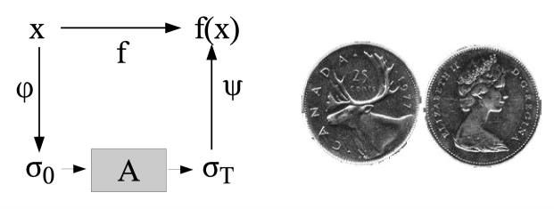
Figure 5: Computing $f$ using a “hard” physical device $A$ (left); a fair coin cannot be considered a “hard” device

Let $f$ be some uncomputable function. Suppose that we had a physical system $A$ and two computable translators $\phi$ and $\psi$, such that $\phi$ translates an input $x$ to $f$ into a state $\phi(x)$ of $A$. The evolution of $A$ on $\sigma_{0}=\phi(x)$ should yield a state $\sigma_{T}$ such that $\psi(\sigma_{T})=f(x)$ (Fig. 5). This means that at least in principle we should be able to build a physical device which would allow us to compute an uncomputable function. To compute $f$ on an input $x$, we translate $x$ into a state $\sigma_{0}=\phi(x)$ of $A$. We then allow $A$ to evolve from state $\sigma_{0}$ to $\sigma_{T}$ – this is the part of the computation that cannot be simulated by a computer. We translate $\sigma_{T}$ to obtain the output $f(x)=\psi(\sigma_{T})$.

To make this scheme practical, we should require $A$ to be robust around $\sigma_{0}=\phi(x)$, at least in some probabilistic sense. That is, for a small random perturbation $\sigma_{0}+\varepsilon$ of $\sigma_{0}$, $\psi(\sigma_{T})$ should be equal to $f(x)$ with high probability.

It is apparent from this discussion that such an $A$ should be hard to simulate numerically, for otherwise $f$ would be computable via a numerical simulation of $A$. On the other hand, “hardness to simulate” does not immediately imply “computational hardness”. Consider for example a fair coin. It is virtually impossible to simulate a coin toss numerically due to the extreme sensitivity of the process to small changes in initial conditions. Despite its unpredictability, a fair coin toss cannot be used to compute “hard” functions, because it is not robust. In fact, due to noise, for any initial conditions which puts the coin far enough from the ground, we know the probability distribution of the outcome: 50% “heads” and 50% “tails”. Another example where “theoretical hardness” of the wave equation does not immediately imply a violation of the CT is presented in [WZ02].

This leads to a question that is essentially equivalent to the CT:

($*$) Is there a robust physical system that is hard to simulate numerically?

This is a question that can be formulated in the framework of bit-computability. Since the only numerical simulations a computer can perform are bit simulations, hardness of some robust system $A$ for the bit model implies a positive answer for $(*)$. On the other hand, proving that all computationally hard systems are inherently highly unstable would yield a negative answer to this question.

Note that even if $(*)$ has a positive answer and CT does not hold, and there exists some physical device $A$ that can compute an uncomputable function $f$, it does not imply that this device could serve some “useful” purpose. That is, it might be able to compute some meaningless function $f$, but not any of the “interesting” undecidable problems, such as solving Diophantine equations or the halting problem.

References

-
[BBY05]
I. Binder, M. Braverman, M. Yampolsky.
On computational complexity of Siegel Julia sets,
arXiv.org e-Print archive, 2005.
Available from
http://www.arxiv.org/abs/math.DS/0502354 - [Blum04] L. Blum, Computing over the Reals: Where Turing Meets Newton. Notices of the Amer. Math. Soc 51, 1024-1034, 2004.
- [BSS89] L. Blum, M. Shub, S. Smale, On a theory of computation and complexity over the real numbers: NP-completeness, recursive functions and universal machines. Bulletin of the Amer. Math. Soc. 21, 1-46, 1989.
- [BCSS98] L. Blum, F. Cucker, M. Shub, S. Smale, Complexity and Real Computation, Springer, New York, 1998.
- [BM75] A. Borodin, I. Munro, The Computational Complexity of Algebraic and Numeric Problems, Elsevier, New York, 1975.
- [Brt03] V. Brattka, The emperor’s new recursiveness: The epigraph of the exponential function in two models of computability. In Masami Ito and Teruo Imaoka, editors, Words, Languages & Combinatorics III, pp. 63-72, Singapore, 2003. World Scientific Publishing. ICWLC 2000, Kyoto, Japan, March 14-18, 2000.
- [BW99] V. Brattka, K. Weihrauch, Computability of Subsets of Euclidean Space I: Closed and Compact Subsets, Theoretical Computer Science, 219, pp. 65-93, 1999.
- [Brv04] M. Braverman, Hyperbolic Julia Sets are Poly-Time Computable. Proc. of CCA 2004, in ENTCS, vol 120, pp. 17-30.
-
[BY04]
M. Braverman, M. Yampolsky. Non-computable Julia sets,
arXiv.org e-Print archive, 2004.
Available from
http://www.arxiv.org/abs/math.DS/0406416 -
[Brv05]
M. Braverman, On the Complexity of Real Functions.
arXiv.org e-Print archive, 2005.
Available from
http://www.arxiv.org/abs/cs.CC/0502066. Accepted for 46th Annual IEEE Symposium on Foundations of Computer Science (FOCS 2005). - [BCS97] P. Burgisser, M. Clausen, M. A. Shokrollahi, Algebraic Complexity Theory. Springer, New York, 1997.
- [DH82] A.Douadyand, J.H.Hubbard, Itération des polynomes quadratiques complexes. C. R. Acad. Sci. Paris, 294, pp. 123-126, 1982.
- [GJ79] M.R. Garey, D.S. Johnson, Computers and Intractability: A Guide to the Theory of NP-Completeness, W.H.Freeman and Company, 1979.
- [Grz55] A. Grzegorczyk, Computable functionals, Fund. Math. 42, pp. 168-202, 1955.
- [Hert05] P. Hertling, Is the Mandelbrot set computable? Math. Logic Quart. 51, issue 1, pp. 5-18, 2005.
- [Ko91] K. Ko, Complexity Theory of Real Functions, Birkhäuser, Boston, 1991.
- [Lac55] D. Lacombe, Classes récursivement fermés et fonctions majorantes, C. R. Acad. Sci. Paris, 240, pp. 716-718, 1955.
- [Lac58] D. Lacombe, Les ensembles récursivement ouverts ou fermés, et leurs applications à l’Analyse récursive, C. R. Acad. Sci. Paris, 246, pp. 28-31, 1958.
- [Mat93] Y. Matiyasevich, Hilbert’s Tenth Problem, The MIT Press, Cambridge, London, 1993.
- [Mil00] J. Milnor, Dynamics in One Complex Variable - Introductory Lectures, second edition, Vieweg, 2000.
- [PR89] M.B. Pour-El, J.I. Richards, Computability in Analysis and Physics, Perspectives in Mathematical Logic, Springer, Berlin, 1989.
- [Ret04] R. Rettinger, A Fast Algorithm for Julia Sets of Hyperbolic Rational Functions. Proc. of CCA 2004, in ENTCS, vol 120, pp. 145-157.
- [RW03] R. Rettinger, K. Weihrauch, The Computational Complexity of Some Julia Sets, in STOC’03, June 9-11, 2003, San Diego, California, USA.
- [Sch82] A. Schönhage, The fundamental theorem of algebra in terms of computational complexity, Technical report, Math. Institut der. Univ. Tübingen, 1982.
- [Sch87] A. Schöhage, Equation solving in terms of computational complexity. In Proceedings of the International Congress of Mathematicians, 1986, A. Gleason, Ed., Amer. Math. Soc., 1987.
- [Shor97] P. Shor, Polynomial-time algorithms for prime factorization and discrete logarithms on a quantum computer. SIAM J. Comput. 26, pp. 1484-1509, 1997.
- [Sma97] S. Smale, Complexity theory and numerical analysis. Acta Numerica, 6, pp. 523-551, 1997.
- [Tur36] A. M. Turing, On Computable Numbers, With an Application to the Entscheidungsproblem. In Proceedings, London Mathematical Society, 1936, pp. 230-265.
- [Wei00] K. Weihrauch, Computable Analysis, Springer, Berlin, 2000.
- [WZ02] K. Weihrauch, N. Zhong, Is wave propagation computable or can wave computers beat the Turing machine? Proc. London Math Soc. (3) 85 pp. 312-332, 2002.
- [Yao02] A. Yao, Classical Physics and the Church-Turing Thesis, Electronic Colloquium on Computational Complexity, Report No. 62, 2002.