Temporal Phylogenetic Networks
and Logic Programming

Abstract

The concept of a temporal phylogenetic network is a mathematical model of evolution of a family of natural languages. It takes into account the fact that languages can trade their characteristics with each other when linguistic communities are in contact, and also that a contact is only possible when the languages are spoken at the same time. We show how computational methods of answer set programming and constraint logic programming can be used to generate plausible conjectures about contacts between prehistoric linguistic communities, and illustrate our approach by applying it to the evolutionary history of Indo-European languages.

1 Introduction

The evolutionary history of families of natural languages is a major topic of research in historical linguistics. It is also of interest to archaeologists, human geneticists, and physical anthropologists. In this paper we show how this work can benefit from the use of computational methods of logic programming.

Our starting point here is the mathematical model of evolution of natural languages introduced in [Ringe et al. (2002)] and [Nakhleh et al. (2005)]. As proposed in [Erdem et al. (2003)], we describe the evolution of languages in a declarative formalism and generate conjectures about the evolution of Indo-European languages using an answer set programming system. Instead of the system smodels, employed in earlier experiments, we make use of the new system cmodels, which leads in this case to much better computation times. Our main conceptual contribution is extending the definition of a phylogenetic network from [Nakhleh et al. (2005)] by explicit temporal information about extinct languages—by estimates of the dates when those languages could be spoken. Computationally, to accommodate this enhancement we divide the work between two systems: cmodels and the constraint logic programming system ecl${}^{\hbox{\scriptsize i}}$ps${}^{\hbox{\scriptsize e}}$ (http://www-icparc.doc.ic.ac.uk/eclipse/).

It was observed long ago (see, for instance, [Gleason (1959)]) that if linguistic communities do not remain in effective contact as their languages diverge then the evolutionary history of their language family can be modeled as a phylogeny—a tree whose edges represent genetic relationships between languages. Fig. 1(a)

$\begin{array}[]{cc}\psfig{}&\psfig{}\\[11.38092pt] \mbox{(a)}&\mbox{(b)}\end{array}$

Figure 1: A temporal phylogeny (a), and a perfect temporal network (b) with a lateral edge connecting $B1$ with $D1$.

shows the extant languages $A$, $B$, $C$, $D$, along with the common ancestor $E$ of $A$ and $B$, the common ancestor $F$ of $C$ and $D$, and the common ancestor $R$ (for “root”) of $E$ and $F$. The time line to the right of the tree shows that the ancestors of $A$ and $B$ diverged around 300 CE, the ancestors of $C$ and $D$ diverged around 800 CE, and the ancestors of $E$ and $F$ diverged around 1000 BCE.

Sometimes languages inherit their characteristics from their ancestors, and sometimes they trade them with other languages when two linguistic communities are in contact with each other. The directed graph in Fig. 1(b), obtained from the tree in Fig. 1(a) by inserting two vertices and adding a bidirectional edge, shows that the ancestor $B1$ of $B$, spoken around 1400 CE, was in contact with the ancestor $D1$ of $D$.

This idea has led Nakhleh, Ringe and Warnow (?) to the definition of a phylogenetic network, which extends the definition of a phylogeny by allowing lateral edges, such as the edge connecting $B1$ with $D1$. The modification of their mathematical model proposed below takes into account the fact that two languages cannot be in contact unless they are spoken at the same time. Geometrically speaking, every lateral edge has to be horizontal. For instance, in Fig. 1(a) there can be no contact between an ancestor of $E$ and a descendant of $F$, although such contacts are not prohibited in the definition of a phylogenetic network. To express the idea of a chronologically possible network in a precise form, we introduce “temporal networks”—networks with a “date” assigned to each vertex. Dates monotonically increase along every branch of the phylogeny, and the dates assigned to the ends of a lateral edge are equal to each other.

Once dates are assigned to the vertices of a phylogeny, we can talk not only about the languages that are represented by the vertices, but also about the “intermediate” languages spoken by members of a linguistic community at various times. In the example above we would represent the language spoken by the ancestors of the linguistic community $A$ at time $t$ by the pair $A\!\!\uparrow\!\!t$, where $300<t<2000$. This pair can be visualized as the point at level $t$ on the edge leading to $A$. In our idealized representation, $t$ ranges over real numbers, so that the set of such pairs is infinite. Language $B1$ in Fig. 1(b) can be denoted by $B\!\!\uparrow\!\!1400$, and $D1$ can be written as $D\!\!\uparrow\!\!1400$.

The characteristics of a language that it could inherit from ancestors or trade with other languages are called (qualitative) characters. A phylogeny describes every leaf of the tree in terms of the values, or “states,” of the characters. For instance, zeroes and ones next to $A$, $B$, $C$ and $D$ in Fig. 1(a) represent the states of a 2-valued character. They can indicate, for example, that a certain meaning is expressed by cognates in languages $A$ and $C$ (cognation class 0), and that it is also expressed by cognates in languages $B$ and $D$ (cognation class 1).

The main definition in this paper (similar to Definition 12.1.3 from [Nakhleh (2004)]) is that of a “perfect” temporal network. A perfect network explains how every state of every qualitative character could evolve from its original occurrence in a single language in the process of inheriting characteristics along the tree edges and trading characteristics along the lateral edges of the network. For instance, Fig. 1(b) extends the phylogeny in Fig. 1(a) to a perfect network by labeling the internal vertices of the graph. Indeed, consider the subgraph of Fig. 1(b) induced by the set $\{A,C,E,F,R\}$ of the vertices that are labeled 0. This subgraph is a tree with the root $R$; this fact shows that state 0 has evolved in this network from its original occurrence in $R$. Similarly, the subgraph of Fig. 1(b) induced by the set $\{B,B1,D,D1\}$ of the vertices labeled 1 contains a tree with the root $B1$, and also a tree with the root $D1$. This means that state 1 could evolve from its original occurrence in language $B1$ (or in an ancestor of $B1$ that is younger than $E$). Alternatively, state 1 could evolve from its original occurrence in language $D1$, or in an ancestor of $D1$ that is younger than $F$.

The computational problem that we are interested in is the problem of reconstructing the temporal network representing the evolution of a language family, such as Indo-European languages. This problem can be divided into two parts: generating a “near-perfect” phylogeny, and then generating a small set of additional horizontal edges that turn the phylogeny into a perfect network. (In a plausible conjecture about the evolution of languages the number of lateral edges has to be small: inheriting characteristics of a language from its ancestors is far more probable than acquiring them through borrowing, unless the dataset includes a large proportion of words that are highly likely to be borrowed.) The first part—generating phylogenies—has been the subject of extensive research; applying answer set programming to this problem is discussed in [Brooks et al. (2005)]. In this paper we address the second part of the problem—turning a phylogeny into a perfect network.

As to the dates assigned to the vertices of the phylogeny, we assume that they are known approximately. For instance, about the graph from Fig. 1(a) we may only know that language $E$ was spoken between 100 BCE and 500 CE, and that language $F$ was spoken between 600 CE and 1100 CE. Since these two intervals do not overlap, we can conclude from these assumptions, just as in the case of the specific dates assigned to $E$ and $F$ in Fig. 1(a), that a contact between an ancestor of $E$ and a descendant of $F$ would be impossible. If, however, the given temporal intervals for $E$ and $F$ were wider then such a conclusion might not be warranted, and a contact between an ancestor of $E$ and a descendant of $F$ might become an acceptable conjecture.

Our method allows us to turn a phylogeny, along with temporal intervals assigned to its vertices, into a perfect network by adding a small number of lateral edges, or to determine that this is impossible.

In this paper, after describing the problem mathematically in Section 2, we show how it can be solved using ideas of answer set programming and constraint logic programming (Section 3), and then apply our approach to the problem of reconstructing the evolutionary history of Indo-European languages (Section 4).

2 Problem Description

In this section we show how the problem of computing perfect temporal phylogenetic networks built on a given temporal phylogeny can be described as a graph problem.

Recall that a rooted tree is a digraph with a vertex of in-degree 0, called the root, such that every vertex different from the root has in-degree 1 and is reachable from the root. In a rooted tree, a vertex of out-degree 0 is called a leaf.

2.1 Temporal Phylogenies

A phylogeny is a finite rooted tree $\langle V,E\rangle$ along with two finite sets $I$ and $S$ and a function $f$ from $L\times I$ to $S$, where $L$ is the set of leaves of the tree. The elements of $I$ are usually positive integers (“indices”) that represent, intuitively, qualitative characters, and elements of $S$ are possible states of these characters. The function $f$ “labels” every leaf $v$—the extant or most recently spoken language in one of the branches—by mapping every index $i$ to the state $f(v,i)$ of the corresponding character in that language.

For instance, Fig. 1(a) is a phylogeny with $I=\{1\}$ and $S=\{0,1\}$. Fig. 2(a) is a phylogeny with $I=\{1,2\}$ and $S=\{0,1\}$; state $f(v,i)$ is represented by the $i$-th member of the tuple labeling leaf $v$.

$\begin{array}[]{cc}\psfig{}&\psfig{}\\[11.38092pt] \mbox{(a)}&\mbox{(b)}\end{array}$

Figure 2: A temporal phylogeny (a), and a perfect temporal network (b) with a lateral edge connecting $B\!\!\uparrow\!\!1750$ with $D\!\!\uparrow\!\!1750$.

A temporal phylogeny is a phylogeny along with a function $\tau$ from vertices of the phylogeny to real numbers such that for every edge $\langle u,v\rangle$ of the phylogeny $\tau(u)<\tau(v)$. Intuitively, $\tau(v)$ is the time when language $v$ was spoken. We will graphically represent the values of $\tau$ by placing a vertical time line to the right of the tree, as in Fig. 1(a) and Fig. 2(a).

2.2 Contacts and Networks

As discussed in the introduction, a contact between two linguistic communities can be represented by a horizontal edge added to a pictorial representation of a temporal phylogeny. The two endpoints of the edge are simultaneous “events” in the histories of these communities. An event can be represented by a pair $v\!\!\uparrow\!\!t$, where $v$ is a vertex of the phylogeny and $t$ is a real number.

To make this idea precise, consider a temporal phylogeny $T$; let $V$ be the set of its vertices, $R$ its root, and $\tau$ its time function. For every $v\in V\setminus\{R\}$, let $\hbox{par\/}(v)$ be the parent of $v$. An event is any pair $v\!\!\uparrow\!\!t$ such that $v\in V\setminus\{R\}$ and $t$ is a real number satisfying the inequalities

$$\tau(\hbox{par\/}(v))<t\leq\tau(v).$$ (1)

Events $v\!\!\uparrow\!\!t$ and $v^{\prime}\!\!\uparrow\!\!t^{\prime}$ are concurrent if $t=t^{\prime}$. A contact is a set consisting of two different concurrent events.

Any finite set $C$ of contacts defines a (temporal phylogenetic) network—a digraph obtained from $T$ by inserting the elements $v\!\!\uparrow\!\!t$ of the contacts from $C$ as intermediate vertices and then adding every contact in $C$ as a bidirectional edge. We will discuss now a simple case that is particularly important for applications, defined as follows.

We say that a set $C$ of contacts is simple if

• for every event $v\!\!\uparrow\!\!t$ that belongs to a contact from $C$, $t<\tau(v)$, and

• for every vertex $v$ of $T$ there exists at most one number $t$ such that $v\!\!\uparrow\!\!t$ belongs to some contact from $C$.

The first condition expresses that the second inequality in (1) holds as a strict inequality, so that for every event $v\!\!\uparrow\!\!t$ that belongs to a contact from $C$

$$\tau(\hbox{par\/}(v))<t<\tau(v).$$ (2)

In other words, it says that the endpoints of all lateral edges are different from the vertices of $T$; each of them subdivides an edge of $T$ into two edges. The second condition says that the endpoints of the lateral edges do not subdivide any of the edges of $T$ into more than two parts. It is clear, for instance, that the set consisting of the single contact

$$\{B\!\!\uparrow\!\!1400,D\!\!\uparrow\!\!1400\}$$ (3)

in Fig. 1 and the set consisting of the single contact

$$\{B\!\!\uparrow\!\!1750,D\!\!\uparrow\!\!1750\}$$

in Fig. 2 are simple.

If $C$ is simple then the corresponding network can be described as follows. The set of its vertices is the union of the set $V$ of vertices of $T$ with the union $V_{C}$ of the contacts from $C$. Its set $E_{C}$ of edges is obtained from the set $E$ of edges of $T$ in two steps. First, for every event $v\!\!\uparrow\!\!t$ in $V_{C}$ we replace the edge $\langle\hbox{par\/}(v),v\rangle$ from $E$ by its “two halves”—the edges

$$\langle\hbox{par\/}(v),v\!\!\uparrow\!\!t\rangle\hbox{ and }\langle v\!\!\uparrow\!\!t,v\rangle.$$

Second, for every contact $\{u\!\!\uparrow\!\!t,v\!\!\uparrow\!\!t\}$ in $C$ we add a “bidirectional lateral edge”—the pair of edges

$$\langle u\!\!\uparrow\!\!t,v\!\!\uparrow\!\!t\rangle\hbox{ and }\langle v\!\!\uparrow\!\!t,u\!\!\uparrow\!\!t\rangle.$$

2.3 Perfect Networks

About a simple set $C$ of contacts (and about the corresponding network $\langle V\cup V_{C},E_{C}\rangle$) we say that it is perfect if there exists a function $g:(V\cup V_{C})\times I\to S$ such that

1. for every leaf $v$ of $T$ and every $i\in I$, $g(v,i)=f(v,i)$;

2. for every $i\in I$ and every $s\in S$, if the set

   $$V_{is}=\{x\in V\cup V_{C}\ :\ g(x,i)=s\}$$

   is nonempty then the digraph $\langle V\cup V_{C},E_{C}\rangle$ has a subgraph with the set $V_{is}$ of vertices that is a rooted tree.

The first condition expresses that the function $g$ extends $f$ from leaves to all ancestral languages of the network. The second condition expresses that every state $s$ of every character $i$ could evolve from its original occurrence in some “root” language.

For instance, Fig. 1(b) shows a perfect network obtained from the phylogeny of Fig. 1(a) by adding one contact, along with labels representing the values of $g$. Similarly, Fig. 2(b) shows a perfect network obtained from the phylogeny of Fig. 2(a) along with the values of the corresponding function $g$. In the last example, state 0 of the first character and state 1 of the second character have evolved from the root of the given phylogeny; state 1 of the first character has evolved from the common ancestor of $B$ and $C$; the state 0 of the second character could evolve from $B\!\!\uparrow\!\!1750$ or from $D\!\!\uparrow\!\!1750$. (Each of these two possibilities corresponds to a subgraph with the vertices $B$, $D$, $B\!\!\uparrow\!\!1750$, $D\!\!\uparrow\!\!1750$ that is a rooted tree.)

2.4 Increment to Perfect Simple Temporal Network

We are interested in the problem of turning a temporal phylogeny into a perfect temporal network by adding a small number of contacts. For instance, given the phylogeny in Fig. 1(a), the single contact (3) is a possible answer.

It is clear that the information included in a temporal phylogeny is not sufficient for determining the exact dates of the contacts that turn it into a perfect network. For instance, if we shift contact (3) up or down by a few hundred years and replace it, say, by

$$\{B\!\!\uparrow\!\!1200,D\!\!\uparrow\!\!1200\}$$

then the new conjecture about the past of the languages $A,B,C,D$ will not be distinguishable from (3).

To make this idea precise, let us select for each $v\in V\setminus\{R\}$ a new symbol $v\!\!\uparrow$, and define the summary of a simple set $C$ of contacts to be the result of replacing each element $v\!\!\uparrow\!\!t$ of every contact in $C$ with $v\!\!\uparrow$. Thus summaries consist of 2-element subsets of the set

$$V\!\!\uparrow=\{v\!\!\uparrow\ :\ v\in V\setminus\{R\}\}.$$

For instance, the summary of the set of contacts of Fig. 1(b) is $\{\{B\!\!\uparrow,D\!\!\uparrow\}\}$. For the set of contacts of Fig. 2(b), the summary is the same. Intuitively, $v\!\!\uparrow$ is a language intermediate between $\hbox{par\/}(v)$ and $v$ that was spoken at some unspecified time between $\tau(\hbox{par\/}(v))$ and $\tau(v)$.

An IPSTN problem (for “Increment to Perfect Simple Temporal Network”) is defined by a phylogeny $\langle V,E,I,S,f\rangle$ and a function

$$v\mapsto(\tau_{\hbox{\scriptsize min\/}}(v),\tau_{\hbox{\scriptsize max\/}}(v))$$

from the vertices of the phylogeny to open intervals. (In other words, for every $v\in V$, $\tau_{\hbox{\scriptsize min\/}}(v)$ is a real number or $-\infty$, and $\tau_{\hbox{\scriptsize max\/}}(v)$ is a real number or $+\infty$, such that $\tau_{\hbox{\scriptsize min\/}}(v)<\tau_{\hbox{\scriptsize max\/}}(v)$.) A solution to the problem is a set of 2-element subsets of $V\!\!\uparrow$ that is the summary of a perfect simple set of contacts for a temporal phylogeny $\langle V,E,I,S,f,\tau\rangle$ such that, for all $v\in V$,

$$\tau_{\hbox{\scriptsize min\/}}(v)<\tau(v)<\tau_{\hbox{\scriptsize max\/}}(v).$$ (4)

Thus a solution is a summary, rather than a set of contacts itself. On the other hand, as discussed in the introduction, an IPSTN problem includes a set of conditions on a time function, rather than a specific temporal phylogeny.

Given an IPSTN problem $Q$ and a nonnegative integer $k$, we want to find the solutions $X$ to $Q$ such that the cardinality of $X$ is at most $k$.

3 Computing Solutions

Our approach to computing solutions is based on their characterization in terms of “admissible sets.” Whether or not a set $X$ is admissible for an IPSTN problem $Q$ is completely determined by the phylogeny of $Q$; this property does not depend on the time intervals $(\tau_{\hbox{\scriptsize min\/}}(v),\tau_{\hbox{\scriptsize max\/}}(v))$. The problem of computing admissible sets lends itself well to the use of answer set programming in the spirit of [Erdem et al. (2003)]. Proposition 1 below shows, on the other hand, that solutions to $Q$ can be described as the admissible sets for which a certain system of equations and inequalities has a solution. This additional condition is easy to verify, for each admissible set, using a constraint programming system.

3.1 Solutions as Admissible Sets

Consider a phylogeny $\langle V,E,I,S,f\rangle$ with a root $R$, and a set $X$ of 2-element subsets of $V\!\!\uparrow$. By $V_{X}$ we denote the union of all elements of $X$. By $E_{X}$ we denote the set obtained from $E$ by replacing, for every $v\!\!\uparrow\in V_{X}$, the edge $\langle\hbox{par\/}(v),v\rangle$ with

$$\langle\hbox{par\/}(v),v\!\!\uparrow\rangle\hbox{ and }\langle v\!\!\uparrow,v\rangle$$

and adding, for every element $\{u\!\!\uparrow,v\!\!\uparrow\}$ of $X$, the edges

$$\langle u\!\!\uparrow,v\!\!\uparrow\rangle\hbox{ and }\langle v\!\!\uparrow,u\!\!\uparrow\rangle.$$

We say that $X$ is admissible if there exists a function $g:(V\cup V_{X})\times I\to S$ such that

1. for every leaf $v$ of the phylogeny and every $i\in I$, $g(v,i)=f(v,i)$;

2. for every $i\in I$ and every $s\in S$, if the set

   $$V_{is}=\{x\in V\cup V_{X}\ :\ g(x,i)=s\}$$

   is nonempty then the digraph $\langle V\cup V_{X},E_{X}\rangle$ has a subgraph with the set $V_{is}$ of vertices that is a rooted tree.

In the following proposition, $Q$ is an IPSTN problem defined by a phylogeny $\langle V,E,I,S,f\rangle$ with a root $R$ and a function $v\mapsto(\tau_{\hbox{\scriptsize min\/}}(v),\tau_{\hbox{\scriptsize max\/}}(v))$.

Proposition 1

A set $X$ of 2-element subsets of $V\!\!\uparrow$ is a solution to $Q$ iff

1. $X$ is admissible, and

2. there exists a real-valued function $\tau$ on $V\cup V_{X}$ such that

   1. for every $v\in V$,

      $$\tau_{\hbox{\scriptsize min\/}}(v)<\tau(v)<\tau_{\hbox{\scriptsize max\/}}(v),$$

   2. for every $v\in V\setminus\{R\}$,

      $$\tau(\hbox{par\/}(v))<\tau(v),$$

   3. for every element $v\!\!\uparrow$ of $V_{X}$,

      $$\tau(\hbox{par\/}(v))<\tau(v\!\!\uparrow)<\tau(v),$$

   4. for every element $\{u\!\!\uparrow,v\!\!\uparrow\}$ of $X$,

      $$\tau(u\!\!\uparrow)=\tau(v\!\!\uparrow).$$

Proof      Left-to-right. Assume that $X$ is a solution to $Q$, so that there exist a real-valued function $\tau$ on $V$ satisfying (4) and a perfect simple set $C$ of contacts for the temporal phylogeny $\langle V,E,I,S,f,\tau\rangle$ such that $X$ is the summary of $C$. The function from $V_{C}$ to $V_{X}$ that maps every event $v\!\!\uparrow\!\!t$ to $v\!\!\uparrow$ is a 1–1 correspondence between the two sets. If we agree to identify every event $v\!\!\uparrow\!\!t$ with its image $v\!\!\uparrow$ under this correspondence then $E_{C}$ becomes identical to $E_{X}$, and the conditions on $g$ in the definition of a perfect set of contacts turn into the conditions on $g$ in the definition of an admissible set. Consequently (i) follows from the fact that $C$ is perfect. To prove (ii), extend $\tau$ from $V$ to $V\cup V_{X}$:

$$\tau(v\!\!\uparrow)=t\ \hbox{ if }\ v\!\!\uparrow\!\!t\in V_{C}.$$

Part (a) follows from (4); part (b) follows from the definition of a temporal phylogeny; part (c) follows from (2); part (d) follows from the definition of a contact.

Right-to-left. Assume that $X$ satisfies conditions (i) and (ii). Consider the temporal phylogeny $T$ that consists of the given phylogeny $\langle V,E,I,S,f\rangle$ and the function $\tau$ restricted to $V$. By (a), $T$ satisfies (4). Let $C$ be the set obtained from $X$ by replacing each symbol $v\!\!\uparrow$ in every element of $X$ with the event $v\!\!\uparrow\!\!t$ where $t=\tau(v\!\!\uparrow)$. From (d) we conclude that the elements of $C$ are contacts; by (c), $C$ is simple. It is clear that $X$ is the summary of $C$. The same reasoning as in the first half of the proof shows that, in view of (i), $C$ is perfect.

3.2 Answer Set Programming

The idea of answer set programming is to represent a given computational problem as a logic program whose answer sets (stable models) [Gelfond and Lifschitz (1988)] correspond to solutions. Systems that compute answer sets for a logic program are called answer set solvers. System smodels with its front-end lparse is one of the most widely used answer set solvers today. The system cmodels is another answer set solver, and it uses lparse as its front-end also. This newer system does not have its own search engine; it is essentially a compiler that translates the problem of computing answer sets into a propositional satisfiability problem (or into a series of propositional satisfiability problems), and invokes a SAT solver, such as zchaff, to perform search.

Unlike Prolog systems, which expect from the user a program and a query, an answer set solver starts computing given a program only. For instance, we can give smodels the input program

p(0).
q(1).
r(X) :- p(X).
r(X) :- q(X).

and it will produce the output

Stable Model: r(0) r(1) q(1) p(0)

—the set of all ground queries to which Prolog would respond yes. Given the program

p(0).
p(1).
q(1-X) :- p(X), not q(X).

smodels responds

Answer: 1
Stable Model: q(1) p(1) p(0)
Answer: 2
Stable Model: q(0) p(1) p(0)

This output means, intuitively, that the program can be understood in two ways: either q(0) is false and q(1) is true, or the other way around. For this program (and for other programs with several answer sets) there is no simple relationship between the behavior of Prolog and the behavior of answer set solvers.

A Prolog program can be viewed as a collection of definitions of predicates. In addition to such “defining” rules, lparse programs often include rules of two other kinds— “choice rules” and “constraints.” For example,

{p,q,r,s}.

is a choice rule. Its answer sets are arbitrary subsets of $\{{\mathtt{p}},{\mathtt{q}},{\mathtt{r}},{\mathtt{s}}\}$. Intuitively, this rule says: for each of the atoms p, q, r, s, choose arbitrarily whether to include it in the answer set. A choice rule may include restrictions on the cardinality of the answer set. For instance, the answer sets of

2 {p,q,r,s} 3.

are the subsets $\{{\mathtt{p}},{\mathtt{q}},{\mathtt{r}},{\mathtt{s}}\}$ whose cardinality is at least 2 and at most 3.

A constraint is, syntactically, a rule with the empty head. The effect of adding a constraint to a program is to make the collection of its answer sets smaller—to remove the answer sets that “violate” the constraint. For instance, by adding the constraint

:- p, not q.

to a program we remove its answer sets that include p and do not include q.

A detailed description of the input language of lparse can be found in the online manual (http://www.tcs.hut.fi/Software/smodels/lparse.ps.gz).

3.3 Generating Admissible Sets

An lparse program for generating admissible sets is shown in Fig. 3.

#domain vertex(U;V).
#domain character(I).
#domain state(S).

{x(UU,VV): vertex(UU;VV): UU != r: VV != r: UU < VV} k.

xx(U,V) :- x(U,V), U < V.
xx(V,U) :- x(U,V), U < V.

v_x(U) :- xx(U,V).

% definition of admissibility, part (i)

g(V,I,S) :- f(V,I,S).
1 {g(V,I,SS): state(SS)} 1 :- e(V,U).
1 {g(pre(V),I,SS): state(SS)} 1 :- v_x(V).

% definition of admissibility, part (ii)

{root(V,I,S)} :- g(V,I,S).
{root(pre(V),I,S)} :- g(pre(V),I,S).

:- root(U,I,S), root(V,I,S), U < V.
:- root(U,I,S), root(pre(V),I,S).
:- root(pre(U),I,S), root(pre(V),I,S), U < V.

reachable(V,I,S) :- root(V,I,S).
reachable(pre(V),I,S) :- root(pre(V),I,S).
reachable(pre(V),I,S) :- e(U,V), g(pre(V),I,S), reachable(U,I,S).
reachable(V,I,S) :- v_x(V), g(V,I,S), reachable(pre(V),I,S).
reachable(V,I,S) :- e(U,V), not v_x(V), g(V,I,S), reachable(U,I,S).
reachable(pre(U),I,S) :- xx(U,V), g(pre(U),I,S), reachable(pre(V),I,S).

:- g(V,I,S), not reachable(V,I,S).
:- g(pre(V),I,S), not reachable(pre(V),I,S).

Figure 3: An lparse program for generating admissible sets.

Table 1 shows the correspondence between the symbols used in the program and the notation introduced in Sections 2,  3.1 and 3.3. The program should be combined with the definition of the domain predicates vertex, e, character, state, f describing the given phylogeny.

The first three lines of the program tell lparse that U and V range over vertices, I ranges over characters, and S over states. The vertices of the phylogeny are assumed to be integers, and the expression U < V in the program is understood accordingly. The verification of condition (ii) from the definition of an admissible set is based on the fact that (ii) can be equivalently stated as follows: for every $i\in I$ and every $s\in S$, if the set $V_{is}$ is nonempty then there is a vertex $v_{is}\in V_{is}$ such all elements of $V_{is}$ are reachable from $v_{is}$ in $V_{is}$ [Erdem et al. (2003), Proposition 1].

Table 1: Explanation of the symbols used in Fig. 3.

lparse program	Mathematical notation
vertex(V)	${\mathtt{V}}\in V$
character(I)	${\mathtt{I}}\in I$
state(S)	${\mathtt{S}}\in S$
e(U,V)	$\langle{\mathtt{U}},{\mathtt{V}}\rangle\in E$
r	$R$
pre(V)	${\mathtt{V}}\!\!\uparrow$
x(U,V)	$\{{\mathtt{U}}\!\!\uparrow,{\mathtt{V}}\!\!\uparrow\}\in X$ and ${\mathtt{U}}<{\mathtt{V}}$
xx(U,V)	$\{{\mathtt{U}}\!\!\uparrow,{\mathtt{V}}\!\!\uparrow\}\in X$
v_x(V)	${\mathtt{V}}\!\!\uparrow\in V_{X}$
f(V,I,S)	$f({\mathtt{V}},{\mathtt{I}})={\mathtt{S}}$
g(V,I,S)	$g({\mathtt{V}},{\mathtt{I}})={\mathtt{S}}$
root(V,I,S)	${\mathtt{V}}=v_{\mathtt{I}S}$
reachable(V,I,S)	V is reachable from $v_{\mathtt{I}S}$ in $V_{\mathtt{I}S}$

The algorithm for solving IPSTN problems suggested by the discussion above consists of two steps: compute admissible sets by running an answer set solver on the program from Fig. 3 and then use a constraint programming system to check, for each of these sets $X$, whether the equations and inequalities from part (ii) of the statement of Proposition 1 have a solution in real numbers $\tau(v)$, $v\in V\cup V_{X}$.

This basic algorithm can be improved using the following observation. Let $X$ be a solution to the given IPSTN problem. Consider the numbers $\tau(v)$ from part (ii) of the statement of Proposition 1. Conditions (a) and (c) imply that for every $v\!\!\uparrow$ in $V_{X}$

$$\tau_{\hbox{\scriptsize min\/}}(\hbox{par\/}(v))<\tau(\hbox{par\/}(v))<\tau(v\!\!\uparrow)<\tau(v)<\tau_{\hbox{\scriptsize max\/}}(v),$$

so that $v\!\!\uparrow$ belongs to the interval $(\tau_{\hbox{\scriptsize min\/}}(\hbox{par\/}(v)),\tau_{\hbox{\scriptsize max\/}}(v))$. In view of (d), it follows that for every element $\{u\!\!\uparrow,v\!\!\uparrow\}$ of $X$, the intervals

$$(\tau_{\hbox{\scriptsize min\/}}(\hbox{par\/}(u)),\tau_{\hbox{\scriptsize max\/}}(u))\hbox{ and }(\tau_{\hbox{\scriptsize min\/}}(\hbox{par\/}(v)),\tau_{\hbox{\scriptsize max\/}}(v))$$

overlap. Consequently, extending the program from Fig. 3 by the constraints

:- x($$u,v$$). (5)

for the pairs $u$, $v$ for which these intervals do not overlap will not lead to the loss of solutions.

3.4 Making the Program Tight

The operation of cmodels [Giunchiglia et al. (2004)] is based on the fact that the answer sets for a program can be described as the models of the program’s completion that satisfy its loop formulas [Lin and Zhao (2002)]. This process is particularly simple in the case when the program is tight, because a tight program has no loops, and its set of loop formulas is empty [Erdem and Lifschitz (2003)], [Lee and Lifschitz (2003), Section 5]. The difference between tight and non-tight programs can be illustrated with a simple example: a program containing the rules

p :- q,r.
q :- p,s.

is not tight, because it contains the loop $\{{\mathtt{p}},{\mathtt{q}}\}$.

The usual recursive definition of the reachability of a vertex in a digraph is tight only when the graph is acyclic. In Fig. 3, the atom reachable(V,I,S) expresses that V can be reached from $v_{\mathtt{I}S}$ in the subgraph of the network induced by $V_{\mathtt{I}S}$; since the network contains cycles, the program in Fig. 3 is not tight.

But we can make this program tight using a transformation somewhat similar to the process of tightening described in [Lifschitz (1996), Section 3.2]. The network is obtained from a tree by adding at most k bidirectional lateral edges. Consequently, the shortest path between any pair of vertices in the network includes at most k lateral edges. Consider the auxiliary atoms rj(V,I,S,J), expressing that there exists a path from $v_{\mathtt{I}S}$ to V in $V_{\mathtt{I}S}$ that contains exactly J lateral edges ($0\leq{\mathtt{J}}\leq{\mathtt{k}}$). The predicate rj can be characterized by a tight definition:

rj(V,I,S,0) :- root(V,I,S).
rj(pre(V),I,S,J) :- root(pre(V),I,S).
rj(pre(V),I,S,J) :- e(U,V), g(pre(V),I,S), rj(U,I,S,J).
rj(V,I,S,J) :- v_x(V), g(V,I,S), rj(pre(V),I,S,J).
rj(V,I,S,J) :- e(U,V), not v_x(V), g(V,I,S), rj(U,I,S,J).
rj(pre(U),I,S,J+1) :- xx(U,V), g(pre(U),I,S), rj(pre(V),I,S,J), J < k.

Then reachable can be defined in terms of rj by the rules

reachable(V,I,S) :- rj(V,I,S,J).
reachable(pre(V),I,S) :- rj(pre(V),I,S,J).

This optimization has a significant effect on the computation time of cmodels.

4 Contacts Between Indo-European Languages

We have applied the concept of a temporal phylogenetic network and the computational methods described above to the problem of generating conjectures about contacts between prehistoric Indo-European languages, discussed earlier in [Nakhleh et al. (2005)], and also in [Erdem et al. (2003)] and [Nakhleh (2004), Chapter 13]. In these experiments, cmodels was used as the answer set solver, and ecl${}^{\hbox{\scriptsize i}}$ps${}^{\hbox{\scriptsize e}}$ as the constraint programming system.

The problems addressed in these experiments are more general than IPSTN problems discussed in Sections 2 and 3: we were interested in sets of contacts that are not necessarily simple in the sense of Section 2.2. The theory and the computational methods presented above have been extended to “IPTN problems” involving the networks that may have several lateral edges meeting the same tree edge, and that may have lateral edges incident to the vertices of the given phylogeny—the possibilities ruled out in the definition of a simple set of contacts. The program shown in Fig. 3 has been modified accordingly, and it was also optimized by allowing function $g$ to be partial, as in [Erdem et al. (2003), Section 5].

4.1 A Phylogeny of Indo-European Languages

As the starting point, we took a phylogeny of Indo-European languages based on the “unscreened IE dataset” published at http://www.cs.rice.edu/$\sim$nakhleh/CPHL/ (without characters that are uninformative or that exhibit known parallel development of states), and on the genetic tree shown in [Nakhleh et al. (2005), Fig. 5] (published originally in [Ringe et al. (2002)]). Using the methods discussed in [Erdem et al. (2003), Sections 3 and 4], we extracted from that phylogeny a small part that appears to contain all components essential for the task of reconstructing contacts between prehistoric Indo-European languages.

The vertices and edges of this smaller phylogeny are shown in Fig. 4.

Figure 4: A phylogenetic tree of Indo-European languages. The languages that do not have commonly accepted names are labeled by numbers.

All vertices except two (Old Church Slavonic and Albanian) are “prehistoric” languages, reconstructed by comparing their descendants. For instance, proto-Celtic has been reconstructed from what is known about its recorded descendants, Old Irish and Welsh (and the fragmentarily attested Continental Celtic languages of antiquity). The phylogeny has 16 qualitative characters (all lexical), and each character has 2 or 3 states. Some of the essential character states are shown in Table 2.

Table 2: The essential character states of some lexical characters for the languages denoted by the leaves of the phylogeny in Fig. 4.

	‘one’	‘arm’	‘beard’	‘free’	‘pour’	‘tear’
proto-Indo-Iranian		5	1			11
proto-Baltic	11	8	5		6	11
Old Church Slavonic			5		6
proto-Greco-Armenian	2		1	3	3	2
proto-Germanic	11	8	5	10	14	2
Albanian	2		1
proto-Italic	11		5	3	14	2
proto-Celtic	11			10		2
proto-Tocharian	2	5			3	11
proto-Anatolian			1

Table 3 shows, for each vertex of the tree, our assumptions about the time when the corresponding language was spoken. Our calculations assume, for instance, that proto-Indo-Iranian was spoken by a generation that lived between 2100 BCE and 1700 BCE.

Table 3: Time intervals for the languages from Fig. 4.

$\;\;v$	$(\tau_{\hbox{\scriptsize min\/}}(v)$,	$\!\!\!\!\tau_{\hbox{\scriptsize max\/}}(v))$
proto-Indo-European	$(-4500$,	$\!\!\!\!-3800)$
proto-Indo-Iranian	$(-2100$,	$\!\!\!\!-1700)$
proto-Balto-Slavic	$(-1400$,	$\!\!\!\!-800)$
proto-Baltic	$(600$,	$\!\!\!\!1000)$
Old Church Slavonic	$(870$,	$\!\!\!\!1000)$
proto-Greco-Armenian	$(-2500$,	$\!\!\!\!-2200)$
proto-Germanic	$(-400$,	$\!\!\!\!0)$
Albanian	$(1800$,	$\!\!\!\!2100)$
proto-Italo-Celtic	$(-3000$,	$\!\!\!\!-2400)$
proto-Italic	$(-1500$,	$\!\!\!\!-1000)$
proto-Celtic	$(-700$,	$\!\!\!\!-300)$
proto-Tocharian	$(-700$,	$\!\!\!\!-300)$
proto-Anatolian	$(-2500$,	$\!\!\!\!-2100)$
Vertex 28	$(-3900$,	$\!\!\!\!-3300)$
Vertex 29	$(-3600$,	$\!\!\!\!-3000)$
Vertex 30	$(-3500$,	$\!\!\!\!-2900)$
Vertex 31	$(-2400$,	$\!\!\!\!-1800)$
Vertex 39	$(-3400$,	$\!\!\!\!-2800)$
Vertex 41	$(-2600$,	$\!\!\!\!-2200)$

Estimating the dates of prehistoric languages is a matter of informed guesswork, because rates of linguistic change are known to vary not only over time but also between lineages (see especially [Bergsland and Vogt (1962)]). Relevant archaeological evidence must be taken into account, but it rarely settles important disputes, because the material remains of a culture typically reveal nothing about the language (or languages) spoken, in the absence of written documents. The dates suggested here for internal nodes of the IE tree are estimates and are presented with considerable diffidence. For a good summary and discussion of the archaeological evidence the reader is referred to [Mallory (1989)].

Some solutions in the sense of Section 2 do not represent viable conjectures about the evolution of Indo-European languages for geographical reasons. For instance, a contact between pre-proto-Celtic and pre-proto-Baltic is unlikely because the former was spoken in western Europe, while the Balts were probably confined to a fairly small area in northeastern Europe. We have eliminated several unrealistic possibilities of this kind at the stage of computing admissible sets, by including additional constraints of the form (5). For instance, the possibility above can be eliminated by adding to the lparse program that generates admissible sets the constraint:

:- x(38,43).

where 38 denotes proto-Celtic and 43 denotes proto-Baltic.

4.2 Results

The problem described in Section 4.1, with the additional geographical constraints mentioned above, turns out to have no solutions consisting of fewer than 3 contacts. There are three solutions of cardinality 3. (To be precise, we should say “three essentially different solutions,” because a summary does not specify the exact times of contacts.) The first (Fig. 5) involves contacts between

pre-Old Church Slavonic and pre-proto-Tocharian,

pre-proto-Germanic and pre-proto-Celtic,

pre-proto-Balto-Slavic and pre-proto-Celtic;

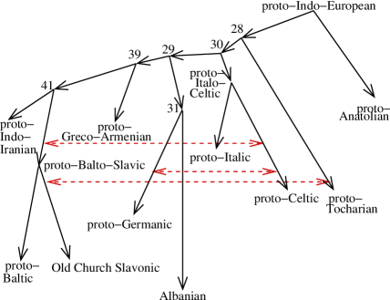
Figure 5: A conjecture about contacts between Indo-European languages generated by cmodels and accepted by ecl${}^{\hbox{\scriptsize i}}$ps${}^{\hbox{\scriptsize e}}$.

the second, contacts between

pre-Old Church Slavonic and pre-proto-Tocharian,

pre-proto-Germanic and pre-proto-Italic,

pre-proto-Italic and pre-proto-Balto-Slavic;

the third, contacts between

pre-proto-Italic and pre-proto-Greco-Armenian,

pre-proto-Germanic and pre-proto-Italic,

pre-proto-Baltic and pre-proto-Germanic.

All three summaries generated by cmodels have been accepted by the ecl${}^{\hbox{\scriptsize i}}$ps${}^{\hbox{\scriptsize e}}$ filter as solutions (which means that all relevant chronological information was expressed in this case by the constraints shown at the end of Section 3.3). They have been computed in about 40 minutes of CPU time using lparse 1.0.13, cmodels 2.10, zchaff Z2003.11.04, and ecl${}^{\hbox{\scriptsize i}}$ps${}^{\hbox{\scriptsize e}}$ 3.5.2, on a PC with a 733 Intel Pentium III processor and 256MB RAM, running SuSE Linux (Version 8.1).

We have also determined, using cmodels, that there exist 193 admissible sets of cardinality 4 that are minimal with respect to set inclusion; out of those, 14 have been rejected by ecl${}^{\hbox{\scriptsize i}}$ps${}^{\hbox{\scriptsize e}}$. Some of the 4-edge solutions represent plausible conjectures about the history of Indo-European languages. One such solution includes, for instance, contacts between

pre-Old Church Slavonic and pre-proto-Tocharian,

pre-proto-Germanic and pre-proto-Italic,

pre-proto-Germanic and pre-proto-Celtic,

pre-proto-Germanic and pre-proto-Baltic.

4.3 Comparison with Earlier Work

The three 3-edge solutions listed in Section 4.2 are identical to the solutions that are marked as “feasible” in [Nakhleh et al. (2005), Table 3]. That table shows the 16 sets of lateral edges generated by MIPPN, the software tool designed for solving the Minimum Increment to Perfect Phylogenetic Network problem. It is different from the computational problem that we solve here using logic programming tools in that its input does not include any chronological or geographical information. The 16 sets of contacts produced by MIPPN were scrutinized by a specialist in the history of Indo-European languages, who has determined that most of them are not plausible from the point of view of historical linguistics. Then the remaining 3 sets were declared feasible. The logic programming approach, on the other hand, allowed us to express the necessary expert knowledge about chronological and geographical constraints in formal notation, and to give this information to the program as part of input, along with the phylogeny. All “implausible” solutions were weeded out in this case by cmodels without human intervention.

In the experiments described in [Erdem et al. (2003)], chronological and geographical information was not part of the input either. But those experiments were similar to the work described in this paper in that search, in both cases, was performed using answer set solvers: smodels in [Erdem et al. (2003)], and cmodels with zchaff in this project. The difference in the computational efficiency between the two engines turned out to be significant. With the new tools available, we did not have to employ the “divide-and-conquer” strategy described in [Erdem et al. (2003), Section 6]. The time needed to compute the 3-edge solutions went down from over 150 hours to around 40 minutes. For comparison, the computation time of MIPPN in the same application was around 8 hours [Nakhleh et al. (2005), Section 5.3].

5 Conclusion

The mathematical model of the evolutionary history of natural languages proposed in [Nakhleh et al. (2005)] enriched the traditional “evolutionary tree” model by allowing languages in different branches of the tree to trade their characteristics. In that theory, phylogenetic networks take place of trees. In this paper we discussed a further enhancement of the phylogenetic network model, which incorporates a real-valued function assigning times to the vertices of the network and prohibits a contact between two languages if it is chronologically impossible. The use of the time function allows us to reduce the number of networks that are mathematically “perfect” but do not represent historically plausible conjectures.

Computing perfect temporal networks can be accomplished by a combination of an answer set programming “generator” with a constraint logic programming “filter.” An alternative approach to combining computational methods developed in these two subareas of logic programming is discussed in [Elkabani et al. (2004)].

In application to the problem of computing perfect networks for a phylogeny of Indo-European languages, the use of cmodels with zchaff has improved the computation time by two orders of magnitude in comparison with the use of smodels in earlier experiments.

References

- Bergsland and Vogt (1962) Bergsland, K. and Vogt, H. 1962. On the validity of glottochronology. Current Anthropology 3, 115–153.
- Brooks et al. (2005) Brooks, D. R., Erdem, E., Minett, J. W., and Ringe, D. 2005. Character-based cladistics and answer set programming. In Proc. PADL-05. 37–51.
- Elkabani et al. (2004) Elkabani, I., Pontelli, E., and Son, T. C. 2004. Smodels with CLP and its application: a simple and effective approach to aggregates in ASP. In Proc. ICLP-04. 73–89.
- Erdem and Lifschitz (2003) Erdem, E. and Lifschitz, V. 2003. Tight logic programs. Theory and Practice of Logic Programming 3, 4–5, 499–518.
- Erdem et al. (2003) Erdem, E., Lifschitz, V., Nakhleh, L., and Ringe, D. 2003. Reconstructing the evolutionary history of Indo-European languages using answer set programming. In Proc. PADL-03. 160–176.
- Gelfond and Lifschitz (1988) Gelfond, M. and Lifschitz, V. 1988. The stable model semantics for logic programming. In Logic Programming: Proceedings of the Fifth International Conference and Symposium, R. Kowalski and K. Bowen, Eds. 1070–1080.
- Giunchiglia et al. (2004) Giunchiglia, E., Lierler, Y., and Maratea, M. 2004. SAT-based answer set programming. In Proc. AAAI-04. 61–66.
- Gleason (1959) Gleason, H. A. 1959. Counting and calculating for historical reconstruction. Anthropological Linguistics 1, 22–32.
- Hock (1986) Hock, H. H. 1986. Principles of Historical Linguistics. Mouton de Gruyter, Berlin.
- Lee and Lifschitz (2003) Lee, J. and Lifschitz, V. 2003. Loop formulas for disjunctive logic programs. In Proc. ICLP-03. 451–465.
- Lifschitz (1996) Lifschitz, V. 1996. Foundations of logic programming. In Principles of Knowledge Representation, G. Brewka, Ed. CSLI Publications, 69–128.
- Lin and Zhao (2002) Lin, F. and Zhao, Y. 2002. ASSAT: computing answer sets of a logic program by SAT solvers. In Proc. AAAI-02. 112–117.
- Mallory (1989) Mallory, J. P. 1989. In Search of the Indo-Europeans. Thames and Hudson, London.
- Nakhleh (2004) Nakhleh, L. 2004. Phylogenetic networks. Ph.D. thesis, University of Texas at Austin. Department of Computer Sciences.
- Nakhleh et al. (2005) Nakhleh, L., Ringe, D., and Warnow, T. 2005. Perfect phylogenetic networks: A new methodology for reconstructing the evolutionary history of natural languages. Language 81, 2, 382–420.
- Ringe et al. (2002) Ringe, D., Warnow, T., and Taylor, A. 2002. Indo-European and computational cladistics. Transactions of the Philological Society 100, 1, 59–129.
- Ross (1997) Ross, M. 1997. Social networks and kinds of speech-community events. In Archaeology and language I: theoretical and methodological orientations, R. Blench and M. Spriggs, Eds. Routledge, London, 209–261.