Mapping DEVS Models onto UML Models

Abstract

Discrete event simulation specification (DEVS) is a formalism designed to describe both discrete state and continuous state systems. It is a powerful abstract mathematical notation. However, until recently it lacked proper graphical representation, which made computer simulation of DEVS models a challenging issue. Unified modeling language (UML) is a multipurpose graphical modeling language, a de-facto industrial modeling standard. There exist several commercial and open-source UML editors and code generators. Most of them can save UML models in XML-based XMI files ready for further automated processing. In this paper, we propose a mapping of DEVS models onto UML state and component diagrams. This mapping may lead to an eventual unification of the two modeling formalisms, combining the abstractness of DEVS and expressive power and “computer friendliness” of the UML.

Keywords: DEVS, UML, state diagram

1.  INTRODUCTION

Discrete event simulation specification (DEVS [?,?,?]) is a powerful formalism for describing discrete event state systems. Various flavors of this formalism have been developed. In this paper, we are using classic DEVS with ports, which we call, simply, DEVS.

Being hierarchical and encapsulated, the DEVS formalism can be naturally implemented in an object-oriented language, such as Java [?]. However, Java-based simulation environments have never been standardized (unlike the DEVS formalism).

An important drawback of the DEVS formalism is the lack of a standardized graphics representation. In [?], an attempt has been undertaken to develop DCharts, a graphics language for DEVS models. DCharts is a UML-based language; however, it does not strictly follow any UML standard. Moreover, the DEVS-to-DCharts transformation proposed in [?] collapses all DEVS states into one DCharts state, essentially eliminating the discrete state nature of DEVS models.

In [?], it is proposed that atomic DEVS models be represented with the help of UML sequence diagrams. However, the sequence diagrams show actual, rather than potential, flow of events. Because of this, a sequence diagram is limited to a particular scenario and cannot unambiguously describe the behavior of a system in its entirety.

An excellent mapping between DEVS models and UML state charts has been introduced in [?]. However, the paper does not suggest a formal mathematical way of constructing the state charts, and thus avoids the issue of the structural clash between DEVS continuous states and UML finite states. It also relies on the older versions of the UML ($<2.0$), which did not have an explicit notion of time.

In this paper, we propose a consistent DEVS-to-UML mapping that takes care of all issues mentioned above. Further restricting the mapping to the executable UML (which is a proper subset of UML [?]) would make a seamless connection between a DEVS model and an UML simulation process, but this topic is beyond the scope of this paper.

2.  DEVS FORMALISM

DEVS supports two complementary models of describing discrete systems: an atomic model that specifies the behavior of an elementary system, and a coupled model that allows us to form more complex models by structurally interconnecting atomic and other coupled models.

A DEVS atomic model is a state machine with input ports $\mathrm{IP}=\{\pi^{in}_{i}\}$ and output ports $\mathrm{OP}=\{\pi^{out}_{i}\}$. Events are associated with input and output ports (they happen at input ports and are generated at output ports). In general, states, unlike events, are not discrete.

2.1.  Atomic Models

Atomic DEVS model $M_{a}$ is a tuple of nine values $M_{a}=\{\mathrm{IP},\mathrm{OP},X,\Sigma,Y,\delta_{\mathrm{in}},\delta_{\mathrm{ext}},\lambda,t_{a}\}$. Here, $\mathrm{IP}$ and $\mathrm{OP}$ are sets of input and output ports.

$\Sigma$ is a set of states $\{\sigma_{i}\}$. A DEVS state $\sigma_{i}$ is uniquely identified with a set of state variables $\gamma_{i}=\{\gamma_{ij}|\sigma_{i}\neq\sigma_{k}\Leftrightarrow\exists j:\gamma_{ij}\neq\gamma_{kj}\}$.

$X$ is a set of input events $\{x_{i}=\left(\pi^{in}_{i},v_{i}\right)\}$, where $\pi^{in}_{i}\in\mathrm{IP}$ is the port name, and $v_{i}$ is the event value. Every event has an associated timestamp, or scheduled time—the time when the event is triggered.

$Y$ is a set of output events {$y_{i}=\left(\pi^{out}_{i},v_{i}\right)\}$, where $\pi^{out}_{i}\in\mathrm{OP}$ is the port name, or the event type, and $v_{i}$ is the event value. $\delta_{\mathrm{int}}\left(\sigma_{i}\right):\Sigma\rightarrow\Sigma$ is the internal transition function. $\delta_{\mathrm{ext}}\left(\sigma_{i},e_{i},x_{j}\right):\left(\Sigma\times R\times\mathrm{IP}\right)\rightarrow\Sigma$ is the external transition function, where $e_{i}$ is the elapsed time in state $\sigma_{i}$. $\lambda\left(\sigma_{i}\right):\Sigma\rightarrow Y$ is the output function. $t_{a}\left(\sigma_{i}\right):\Sigma\rightarrow R$ is the time advance function.

The semantics of the model are as follows: the system stays in state $\sigma_{i}$ for $t_{a}\left(\sigma_{i}\right)$ time units (until a timeout event) or until an external event happens, whatever comes first. In the case of an external event $x_{j}$, the system changes its state to $\delta_{\mathrm{ext}}\left(\sigma_{i},e_{i},x_{j}\right)$. In the case of a timeout, the system changes its state to $\delta_{\mathrm{int}}\left(\sigma_{i}\right)$ and generates an event of type $\lambda\left(\sigma_{i}\right)$. In either case, the simulation time is implicitly advanced to the timestamp of the event that triggered the transition. The initial state of the model is not defined explicitly.

2.2.  Coupled Models

Coupled models are used to compose atomic and other coupled models to produce more DEVS models in a hierarchical way (Figure 1).

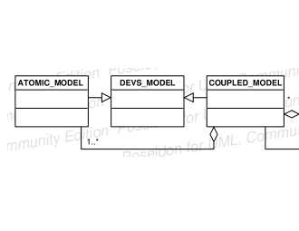
Figure 1.: Atomic and coupled DEVS models

Coupled DEVS model $N$ is a tuple of ten values $N=\{\mathrm{IP},\mathrm{OP},X,Y,D,M,E_{IC},E_{OC},I_{C},S\}$. Here, $\mathrm{IP}$ and $\mathrm{OP}$ are sets of external (not coupled) input and output ports. $X$ is a set of input events $x_{i}=\left(\pi^{in}_{i},v_{i}\right)$, where $\pi^{in}_{i}\in IP$ is the port name, and $v_{i}$ is the event value, and $Y$ is a set of output events $y_{i}=\left(\pi^{out}_{i},v_{i}\right)$, where $\pi^{out}_{i}\in OP$ is the port name, and $v_{i}$ is the event value.

$D=\{d_{i}\}$ is a set of references to the coupled components (atomic models or other coupled models), and $M=\{M_{d}|d\in D\}$ is a set of the coupled components. $E_{IC}\subseteq\{((N,\mathrm{IP}_{i}),(d,\mathrm{IP}_{di}))|\mathrm{IP}_{i}\in\mathrm{IP},d\in D,\mathrm{IP}_{di}\in\mathrm{IP}_{d}\}$ is external input coupling that connects external input ports of the coupled model to the components’ input ports $\mathrm{IP}_{d}$. $E_{OC}\subseteq\{(d,\mathrm{OP}_{di}),((N,\mathrm{OP}_{i}))|\mathrm{OP}_{i}\in\mathrm{OP},d\in D,\mathrm{OP}_{di}\in\mathrm{OP}_{d}\}$ is external output coupling that connects components’ output ports $\mathrm{OP}_{d}$ to the external output ports of the coupled model.

$I_{C}=\{((a,\mathrm{OP}_{ai}),(b,\mathrm{IP}_{bj}))|a,b\in D,\mathrm{OP}_{ai}\in\mathrm{OP}_{a},\mathrm{IP}_{bj}\in\mathrm{IP}_{b}\}$ is internal coupling that interconnects output and input ports of the components. Finally, $S:\{\epsilon_{d}|d\in D\}\rightarrow\epsilon_{d}$ is a selection function that resolves potential scheduling conflicts, when more than one event in different components has the same scheduled time.

Under the principle of closure, a coupled model looks externally like an atomic model and can be used anywhere in place of an atomic model.

A coupled model is simulated as an ensemble of its DEVS components. Output events generated by each individual component are propagated to the input ports of other coupled components or to the output ports of the model, according to the functions $I_{C}$ and $E_{OC}$. In the former case, they are also converted into appropriate input events. Input events received by the model are propagated to the input ports of its components, according to the function $E_{IC}$.

Classic DEVS formalism does not permit feedback loops: $((d,\mathrm{OP}_{di}),(e,\mathrm{OP}_{ej}))\in I_{C}\Rightarrow d\neq e$.

3.  UML FORMALISM

The Unified Modeling Language (UML [?]), a de-facto industrial modeling standard, seems to be a natural choice for a visual representation of DEVS. Besides being widely supported by both proprietary and open-source tools (such as Rose [?] and Poseidon [?]), it also has an associated XML-based representation, XMI, that makes it possible to process UML diagrams by application programs.

Of particular interest for us are UML state and component diagrams, which will be discussed in detail.

3.1.  State Diagrams

A UML state diagram (also known as a statechart, Figure 2) is a visual representation of a finite state automaton with history. Many of the features of state diagrams, such as “do” activities, history states, junction and choice states, concurrent and composite states, are not essential for DEVS-to-UML mappings and will not be considered.

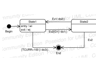
Figure 2.: A UML state diagram

A state diagram is a tuple $SD=\{S,S^{\bullet},S^{\odot},P,T\}$.

Here $S=\{s_{i}=(G_{i},w_{i},q_{i})\}$ is a set of finite states. UML finite states are enumerated using state variable $G$, such that $s_{i}=s_{j}\Leftrightarrow G_{i}=G_{j}$. $w_{i}(x):\mathrm{any}\rightarrow\mathrm{None}$ is an “entry” action. This action is executed just after changing the current state of the model to $s_{i}$. $q_{i}(x):\mathrm{any}\rightarrow\mathrm{None}$ is an “exit” action. This action is executed just before changing the current state of the model from $s_{i}$ to some other state.

A set of possibly continuous pseudostate variables $H=\{h_{k}\}$ ($|H|\geq 0$) extends the definition of a UML state. The pseudostate variables may or may not have different values in different states. They cannot be used to distinguish UML states in a state diagram. An optional class diagram of the UML system can be used to record these variables in the model (Figure 3).

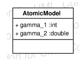
Figure 3.: A UML class diagram that consists of only one class definition. Notice that, formally, variables of types int and double are finite, because both classes have limited range and cardinality.

$S^{\bullet}=\{s_{i}\in S\}$ is the set of the initial states of the diagram. Every diagram can have at most one initial state. Because DEVS formalism does not specify the initial state of the system, we will assume that in general $S^{\bullet}=\emptyset$.

$S^{\odot}=\{s_{i}\in S\}$ is the set final (terminal) states of the diagram. Because the final state of a DEVS system is not defined, we will assume that in general $S^{\odot}=\emptyset$.

$P=\{p_{j}\}$ is a set of discrete events. Each event $p_{j}$ has the associated scheduled time $\tau_{j}$ and a possibly empty set of other attributes.

Finally, $T=\{s_{bi},s_{ei},p_{i},g_{i},a_{i}|s_{bi},s_{ei}\in S,p_{i}\in P,g_{i}\left(x\right):\mathrm{range}(x)\rightarrow\{\mathrm{True},\mathrm{False}\},a_{i}(y):\mathrm{any}\rightarrow\mathrm{None}\}$ is a set of transitions. In UML notation, a transition from state $s_{bi}$ to state $s_{ei}$ on event $p_{i}$ with guard condition $g_{i}$ is denoted as $p_{i}\left[g_{i}\right]/a_{i}$. Action $a_{i}$ is executed just before the completion of the transition. The action is not allowed to change the UML state of the system.

The semantics of a UML state diagram prescribes that in the course of transition $t_{i}$ from state $s_{j}$ to state $s_{k}$ the “exit” action $q_{j}$ is executed first, followed by the transition action $a_{i}$, followed by the “entry” action $w_{k}$.

3.2.  Component Diagrams

UML component diagrams have evolved substantially from version 1.x of the language to the current 2.0 [?,?]. The direction of the evolution has favored the DEVS-to-UML mapping we are about to propose.

In the latest version of the language, deployment, object, and component diagrams have been merged into a single class of deployment/object/component (DOC) diagrams. These new DOC diagrams have a rich language suitable for elaborated models, but for the purpose of this paper we need to mention only components, interfaces, and ports.

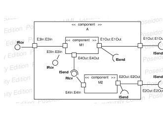
Figure 4.: A UML component diagram

A UML component diagram is a tuple $N^{u}=\{M^{u},Q^{u},E^{u}_{C},I^{u}_{C}\}$.

Here, $M^{u}=\{M^{u}_{i}\}$ is a list of components in the diagram. Each component $M^{u}_{i}$ has list $P^{u}_{i}=\{p_{ij}=(t_{ij},if_{ij},d_{ij})\}$ of externally visible ports. A UML port $p$ has a type. The type of the port specifies the names of the signals (events) that are acceptable through this port. For the purpose of this paper, we assume that the type $t$ of the port is the same as its name. A port can be unidirectional (input or output) or bidirectional. The direction of the port $\mathrm{dir}(p_{ij})$ is defined by the type(s) of its interfaces. Since DEVS formalism does not support bidirectional ports, we will not consider them and consider only one interface $K=(n,d)$ per port, where $n$ is the name of the interface and $d=\{\mathrm{required}|\mathrm{provided}\}$ is its type. Required interfaces (“antennas”) define output ports, and provided interfaces (“lollipops”) define input ports.

A UML component represents either another UML component diagram, or a UML state diagram.

Set $Q^{u}\subseteq\{(M^{u}_{i},M^{u}_{j})|M^{u}_{i}\subset M^{u}\wedge M^{u}_{j}\subset M^{u}\}$ defines the containment relation: component $M$ is a subcomponent of component $N$, or a nested component, if $(N,M)\in Q^{u}$. Let $Z(N)=\{M_{i}|M_{i}\in M^{u}\wedge((N,M_{i})\in Q^{u}\vee(\exists M_{j}:M_{j}\in Z(N)\wedge(M_{j},M_{i})\in Q^{u})\}$ be the set of children of $N$. The containment relation must satisfy additional conditions: (a) a component cannot be a subcomponent of itself: $\forall M\in M^{u}:(M,M)\not\in Q^{u}$ and (b) if $M$ is a subcomponent of component $N$, then $N$ cannot be a subcomponent of $M$ or of any child of $M$: $(N,M)\in Q^{u}\leftrightarrow(M,N)\not\in Q^{u}\wedge\forall M^{\prime}\in Z(M):(M^{\prime},N)\not\in Q^{u}$.

Components $T_{N^{u}}=\{T_{i}|T_{i}\in M^{u}\wedge\forall M\in M^{u}:(T_{i},M)\not\in Q^{u}\}$ are called top-level components. The set:

$$\begin{split}E^{u}_{C}&\subseteq\{((M_{i},p_{ik}),M_{j},p_{jl}))|\\ &M_{i}\in M^{u}\wedge M_{j}\in M^{u}\wedge\\ &(M_{i},M_{j})\in Q^{u}\wedge\\ &p_{ik}\in P^{u}_{i}\wedge p_{jl}\in P^{u}_{j}\wedge\\ &\mathrm{dir}(p_{ik})=\mathrm{dir}(p_{jl})\}\end{split}$$ (1)

is the external coupling that connects external ports of the component to the subcomponents’ ports using UML delegation connectors. External ports must be connected to the internal ports of the same direction. The set:

$$\begin{split}I^{u}_{C}&\subseteq\{((M_{i},p_{ik}),(M_{j},p_{jl}))|\\ &M_{i}\in M^{u}\wedge M_{j}\in M^{u}\wedge\\ &\exists M_{p}\in M^{u}:\{(M_{i},M_{p}),(M_{j},M_{p})\}\subseteq Q^{u}\wedge\\ &p_{ik}\in P^{u}_{i}\wedge p_{jl}\in P^{u}_{j}\wedge\\ &\mathrm{dir}(p_{ik})\neq\mathrm{dir}(p_{jl})\}\end{split}$$ (2)

is the internal coupling that interconnects ports of the subcomponents of the same component using UML assembly connectors. Internal ports must be connected to the internal ports of the opposite direction. Graphically, this is accomplished by matching “antennas” and “lollipops”.

A simple UML component diagram (strictly speaking, a DOC diagram) is shown in Figure 4. It depicts two components M1 and M2. These components are in turn subcomponents of component A. Component A has two output ports E1Out and E2Out with interface ISend and one input port E3In with interface IRcv. The output ports of subcomponents M1 and M2 are connected to the corresponding output ports of the component A, the input port of A is connected to the input port of subcomponent M1. Finally, the output port E4Out of component M1 with interface ISend is connected to the input port E4In of component M2 with interface IRcv.

Composite structure diagrams, which only recently have become a part of the UML 2.0 proposal [?], offer even better mapping between DEVS models and UML models. However, the discussion of these diagrams is beyond the scope of this paper.

4.  ATOMIC DEVS AND UML STATE DIAGRAMS

To map an atomic DEVS model into an UML state diagram, we need to map states, ports, transitions, and outputs.

4.1.  States

In general, DEVS states are neither discrete nor finite, while UML states are always discrete and finite. To map a DEVS system onto an UML system, the DEVS state must be discretized. This can be done by rearranging and grouping DEVS state variables $\gamma=\{\gamma_{j}\}$ according to their kind. Discrete and finite variables can be collected in one subgroup, and countable and continuous variables—into another subgroup:

$$\begin{split}\gamma=(\underbrace{\gamma_{1},\ldots,\gamma_{m}},\underbrace{\gamma_{m+1},\ldots,\gamma_{n}}),&1\leq m\leq n\\ |\mathrm{range}(\gamma_{j})|<\infty,&1\leq j\leq m\\ |\mathrm{range}(\gamma_{j})|=\infty,&m<j\leq n\\ \end{split}$$ (3)

Let’s call the first group finite DEVS state variables, and the other group free DEVS state variables.

For any feasible combination of values of finite DEVS state variables $\{\gamma_{i}|1\leq i\leq m\}$, a UML finite state can be constructed by simply enumerating this combination: $G_{j}=\bigotimes_{i=1}^{m}\gamma_{i}$, where the details of the function $\bigotimes$ are not important as long as it always maps distinct combinations of finite DEVS state variables onto distinct UML states.

All remaining DEVS free state variables $\{\gamma_{i}|m<i\leq n\}$ are mapped to UML pseudostate variables $H=\{h_{i}|1\leq i<n-m\}$ one-to-one. They become attributes of finite states and will be manipulated during DEVS state transitions.

In the case of $m=0$ a DEVS model has no finite state variables, and partitioning (3) is not possible. The UML state diagram will have only one final state. This case is presented in [?].

On the other hand, when $m=n$, the DEVS model has no free variables. Every feasible combination of the DEVS state variables maps onto a UML finite state, and the UML model has no pseudostate variables.

Not being a dynamic simulation language, UML does not enforce an explicit notion of time in all types of diagrams. In particular, UML state diagrams do not have explicit time. The simulation time has to be maintained implicitly, with model-wide variable $t_{\mathrm{curr}}$ denoting the current simulation time.

For the purpose of computing state transitions, many DEVS models depend on the time $e_{i}$ spent by the model in state $\sigma_{i}$. To accommodate this need, we introduce another model-wide variable $t_{e}$—the time of the most recent state transition. An “entry” action $w_{i}$ can be added to every UML finite state that records the value of $t_{e}$:

def $w_{i}$ ():
         $t_{e}=t_{\mathrm{curr}}$

At any given time, the value of $e_{i}$ can be now computed as:

$$e_{i}=\begin{cases}t_{\mathrm{curr}}-t_{e}&\text{if $i$ is the current state,}\\ +\infty&\text{otherwise.}\end{cases}$$ (4)

4.2.  Ports

DEVS input and output ports are mapped to UML events one-to-one:

$$\forall\pi_{i}\in\left(\mathrm{IP}\cup\mathrm{OP}\right)\exists!p_{j}\in P.$$

Input and output events are not distinguished in UML state diagrams.

DEVS formalism does not specify whether the same port can be used as an input port and an output port (whether $\mathrm{IP}\cap\mathrm{OP}=\emptyset$). We will assume that the DEVS ports are indeed unidirectional. This means that an event of a certain type can be only consumed or produced by a state diagram, but not both.

4.3.  External Transitions

The heterogeneous structure of DEVS states and UML states produces heterogeneous structures of DEVS and UML state transitions. Among other things, a single DEVS external transition function $\delta_{\mathrm{ext}}\left(\sigma_{i},e_{i},x_{j}\right)=(\pi^{in}_{j},\nu_{j})$ has to generate both proper UML state transitions and their associated guard conditions and actions.

The total state $S_{T_{i}}$ of a UML model is defined by the current UML finite state and the values of the pseudostate variables:

$$S_{T_{i}}\equiv\left(s_{i},H\right),|H|=n-m+1.$$

The total state $\Sigma_{i}$ of a DEVS model is defined by the values of all DEVS state variables:

$$\Sigma_{i}\equiv\left(\gamma_{i1},\ldots,\gamma_{in}\right)=\gamma_{i}.$$

To reflect a transition from a DEVS state $\sigma_{i}$ to another state $\sigma_{j}$, the corresponding UML model has to change from a UML state $s_{i}=f(\gamma_{i})$ to another UML state $s_{j}=f(\sigma_{j})$ and also update the values of the pseudostate variables: $H_{j}=f(\gamma_{j})$. Here, $f(\chi):\mathrm{DEVS\_objects}\rightarrow\mathrm{UML\_objects}$ is the polymorphic mapping function from the universe of DEVS objects to the universe of UML objects which has been partially defined above.

Action $a^{e}_{l}$ associated with a possible UML transition $t_{l=(ijk)}=\{s_{i},s_{j},p_{k},g^{e}_{l},a^{e}_{l}\}$ from state $s_{i}$ to state $s_{j}$ on event $p_{k}=f(\pi^{in}_{k})$ would be responsible for updating the values of pseudostate variables $H$. It may depend on the original values of the pseudostate variables, on the value of the event, and on $e_{i}$:

def $a^{e}_{l}$ ($H_{i}$, $\nu_{k}$, e):
         $H_{j}$=$z^{e}_{l}$($H_{i}$, $\nu_{k}$, e)

Here, $z^{e}_{l}(H,\nu,e)$ is the explicit state update function:

$$\begin{split}z^{e}_{l}(H,\nu,e)&=H^{\prime}\leftrightarrow\\ &e\geq 0\wedge\\ &\delta_{\mathrm{ext}}\left(\left(s_{i},H\right),e,(\pi^{in}_{k},\nu)\right)=\left(s_{j},H^{\prime}\right).\end{split}$$ (5)

This function may be undefined for some or all values of $H$, $\nu$, and $e=e_{i}$. A condition for a possible UML transition is set $C^{e}_{l}$ constructed in the following way:

$$C^{e}_{l}=\{\left(H,\nu,e\right)|(H,\nu,e)\in\mathrm{dom}(z^{e}_{l})\}.$$ (6)

The UML transition exists if and only if the corresponding condition is not an empty set:

$$t_{l}\in T\leftrightarrow C^{e}_{l}\neq\emptyset.$$

Note that multiple transitions from $s_{i}$ to $s_{j}$ may exist for different events $x_{k}$. In general, $s_{i}$ can be the same state as $s_{j}$ (loopback transitions are possible).

The guard condition $g_{k}$ is a functional representation of the condition set $C^{e}_{l}$:

$$g^{e}_{l}(H,\nu,e)=\begin{cases}\mathrm{true}&(H,\nu,e)\in C^{e}_{l},\\ \mathrm{false}&\text{otherwise},\end{cases}$$ (7)

where $e$ for state $s_{i}$ is defined by Eq. 4. The transition is “fired” if event $p_{k}$ occurs and $g^{e}_{l}(H,\nu_{k},e)$ is true.

4.4.  Internal Transitions and Output Events

Internal transitions and generation of output events are regulated by the internal transition function $\delta_{\mathrm{int}}\left(\sigma_{i}\right)$, the time advance function $t_{a}\left(\sigma_{i}\right)$, and the output function $\lambda\left(\sigma_{i}\right)$. The three functions coöperate in the sense that the first function computes the target state of the transition, the second schedules the transition, and the third generates an output event associated with the transition. DEVS models allow to output events only during internal transitions.

As the external UML transitions, internal UML transitions need to advance the UML model to another state and to update the pseudostate variables.

Action $a^{i}_{l}$ associated with a possible UML transition $t_{l=(ijk)}=\{s_{i},s_{j},\epsilon,g^{i}_{l},a^{i}_{l}\}$ from state $s_{i}$ to state $s_{j}$ on null event $\epsilon$ would be responsible for updating the values of pseudostate variables $H$. It may depend on the original values of the pseudostate variables.

Unlike an action associated with an external transition, $a^{i}_{l}$ can generate output events. UML2.0 allows UML components to “send” events to any UML component $M$, including the component that sends the event (“self”), either immediately, or later. Keyword “after” that is used to schedule an event in the future. Caret (^) represents the send operation. For example, ^M.e after $t$ means “send event $e$ to component $M$ after time $t$.”

The function $\lambda\left(\sigma_{i}\right)$ defines whether an output event is generated during the transition or not, and if yes, what is the type (port) of the event $\pi^{out}_{i}$ and its value $\nu_{i}$. The value of the event can be stored in the UML model as its attribute. By construction, the name of the output event and the name of the output port of an atomic DEVS model coincide:

def $a^{i}_{l}$ ($H_{i}$):
         ($\pi^{out}_{i},\nu_{i}$)=$\lambda\left(\sigma_{i}\right)$
         ^$\pi^{out}_{i}.\left(\pi^{out}_{i}(\nu_{i})\right)$
         $H_{j}$=$z^{i}_{l}$($H_{i}$)

Here, $z^{i}_{l}(H)$ is the explicit state update function for internal transitions:

$$z^{i}_{l}(H)=H^{\prime}\leftrightarrow\delta_{\mathrm{int}}\left(\left(s_{i},H\right)\right)=\left(s_{j},H^{\prime}\right).$$ (8)

This function may be undefined for some or all values of $H$. A condition for a possible internal UML transition is set $C^{i}_{l}$ constructed in the following way:

$$C^{i}_{l}=\{H|H\in\mathrm{dom}(z^{i}_{l})\}.$$ (9)

The internal UML transition exists if and only if the corresponding condition is not an empty set:

$$t_{l}\in T\leftrightarrow C^{i}_{l}\neq\emptyset.$$

In general, $s_{i}$ can be the same state as $s_{j}$ (internal loopback transitions are possible).

The guard condition $g_{k}$ is a functional representation of the condition set $C^{i}_{l}$:

$$g^{i}_{l}(H)=\begin{cases}\mathrm{true}&H\in C^{i}_{l},\\ \mathrm{false}&\text{otherwise},\end{cases}$$ (10)

The time spent in DEVS state $\sigma_{i}$ before the transition is scheduled, is given by the function $t_{a}\left(\sigma_{i}\right)$.

It is tempting to use the send/after apparatus to schedule the transition in the future. However, a transition is not an event and cannot be scheduled using “after” and “send”. Instead, we declare new timeout event $e_{i}$ and schedule it at time $t_{\mathrm{curr}}+t_{a}((s_{i},H_{i}))$ be redefining the entry action $w_{i}$ of state $s_{i}$.

Event $e_{i}$ becomes the trigger for the internal transition from state $s_{i}$.

A situation may occur when a timeout event has been scheduled, and an external transition is triggered by another (input) event. In this case, the pending timeout must be canceled. UML2.0 does not allow to recall scheduled events. Instead, a guard condition can be changed to make sure that obsolete timeouts do not trigger internal transitions.

Let every UML state $s_{i}$ have local variable $y_{i}$ initialized to the reference to the most recently scheduled timeout event $e_{i}$ in the entry action:

def $w_{i}$ ():
         $t_{e}=t_{\mathrm{curr}}$
         $y_{i}=\mathrm{ref}(e_{i})$
         ^self.$e_{i}$ after $t_{a}((s_{i},H_{i}))$

If the value of $y_{i}$ and the reference to the scheduled timeout $e_{i}$ differ, the timeout event must be ignored.

To summarize, an internal transition from state $s_{i}$ is scheduled when $e_{i}$ occurs and if $\left(y_{i}==\mathrm{ref}(e_{i})\right)\wedge g^{i}_{l}(H)$ is true.

5.  COUPLED DEVS AND UML COMPONENT DIAGRAMS

DEVS coupled models and UML component diagrams have a very similar structure, which makes mapping DEVS models onto UML component diagrams rather straightforward.

5.1.  Components

A DEVS coupled model $N$ has only one top-level component and only one level of nesting. This corresponds to a UML component diagram $N^{u}$ with $T_{N}=\{T_{0}\}$ and such that $\forall M_{i}\in M^{u}\setminus T_{N},\forall M_{j}\in M^{u}:(M_{i},M_{j})\not\in Q^{u}$.

The top-level component $T_{0}$, therefore, represents the DEVS coupled model itself, and for each DEVS component $M_{d}\in M$ there exists an UML component $M^{u}_{i}\in M^{u},M^{u}_{i}=f(M_{d})$.

5.2.  Ports

Both input ports $\mathrm{IP}$ and output ports $\mathrm{OP}$ of $N$ are mapped to the corresponding UML ports of the top-level component $T_{0}$ with externally visible ports $P^{u}_{0}$. Let port $p_{i}\in\mathrm{IP}$ carry input events of type $x_{i}\in X$. Then for this port $\exists p^{u}_{i}=f(p_{i})=(t,i\!fc,d)\in P^{u}_{0}:d=\mathrm{input}\wedge t=x_{i}$. Let port $p_{j}\in\mathrm{OP}$ carry output events of type $y_{j}\in Y$. Then for this port $\exists p^{u}_{j}=f(p_{j})=(t,i\!fc,d)\in P^{u}_{0}:d=\mathrm{output}\wedge t=y_{j}$. Notice that input and output events are mapped to the port names implicitly.

5.3.  Connectors

External DEVS coupling corresponds to external (delegation) UML connectors. External input coupling of input port $p_{i}\in\mathrm{IP}$ to an input port $p^{u}_{j}=f(p_{i})$ of component $M_{d}\in M$ is mapped to a delegation connector from the corresponding port of $T^{u}_{0}$ to the corresponding port of $M^{u}_{i}$: $\forall c_{i}=((N,\mathrm{IP}_{i}),(d,\mathrm{IP}_{di}))\in E_{IC}\exists c^{u}_{j}=((T_{0},p_{0j}),(M^{u}_{k},p_{kl})):M^{u}_{k}=f(M_{d})\wedge p_{0j}=f(\mathrm{IP}_{i})\wedge p_{kl}=f(\mathrm{IP}_{di})$. Respectively, external output coupling of an output port $p^{u}_{j}=f(p_{i})$ of component $M_{d}\in M$ to output port $p_{i}\in\mathrm{OP}$ is mapped to a delegation connector from the corresponding port of $M^{u}_{i}$ to the corresponding port of $T^{u}_{0}$: $\forall c_{i}=((d,\mathrm{OP}_{di}),(N,\mathrm{OP}_{i}))\in E_{OC}\exists c^{u}_{j}=((M^{u}_{k},p_{kl}),(T_{0},p_{0j})):M^{u}_{k}=f(M_{d})\wedge p_{0j}=f(\mathrm{OP}_{i})\wedge p_{kl}=f(\mathrm{OP}_{di})$.

Internal DEVS coupling corresponds to internal (assembly) UML connectors. Internal coupling of port $p^{u}_{j}=f(p_{i})$ of component $M_{d}\in M$ to port $p^{u}_{l}=f(p_{k})$ of component $M_{e}\in M$ is mapped to an assembly connector from the corresponding port of $M^{u}_{i}=f(M_{d})$ to the corresponding port of $M^{u}_{k}=f(M_{e})$.

5.4.  Selection function

There is no feasible way of mapping the DEVS selection function to a UML model. Fortunately, parallel DEVS models do not use this function at all.

6.  CONCLUSION AND FUTURE WORK

In the paper, we proposed a mapping of discrete event specification (DEVS) models onto Unified Modeling language (UML) state and component diagrams. This diagrams are designed and optimized for computerized processing and are highly expressive, competitive, and widely used both in academia and industry. Successful automated DEVS-to-UML mapping techniques would enable seamless integration of the legacy of DEVS models into existing and emerging UML models.

As the future step, we plan to consider UML2.0 composite structure diagrams as more suitable representations of DEVS coupled models. An automated translator from the DEVS domain into the UML domain would substantially simplify the transformation. Limiting the output to the Executable UML is also considered.

7.  BIOGRAPHY

Dr. D. Zinoviev received his Ph.D. in Computer Science from SUNY at Stony Brook in 1997. He was working as a post-doc on the DARPA/NASA/NSA-sponsored Petaflops project of a hybrid technology, multi-threaded hypercomputer. In 2000, he joined the Computer Science Department of Suffolk University in the rank of Assistant Professor. His current research interests include simulation and modeling (network simulation, architectural simulation), operating systems, and software engineering.

References

- [1] G. Booch, J. Rumbaugh, and I. Jacobson. The Unified Modeling Language. User Guide. Addison Wesley, 1999.
- [2] H. Feng. DCharts, a formalism for modeling and simulation based design of reactive software systems. Master’s thesis, School of Computer Science, McGill University, Montréal, Canada, February 2004.
- [3] GentleWare. Poseidon for UML community edition v. 2.5.1. Available at http://gentleware.com.
- [4] J. Hogg. UML 2.0 automates code generation from architecture. COTS Journal, May 2004. Available online at http://www.cotsjournalonline.com.
- [5] S.-Y. Hong and T. G. Kim. Embedding UML subset into object-oriented DEVS modeling process. In A. Bruzzone and E. Williams, editors, Proc. SCSC 2004, pages 161–166, San Jose, CA, July 2004.
-
[6]
IBM.
Rational rose.
Available at
http://ibm.com/software/rational/. - [7] S. J. Mellor and M. J. Balcer. Executable UML: A Foundation for Model Driven Architecture. Addison-Wesley, 2002.
- [8] J. Rumbaugh, I. Jacobson, and G. Booch. The Unified Modeling Language Reference Manual. Addison Wesley, second edition, 2004.
- [9] H. Sarjoughian and R.K. Singh. Building simulation modeling environments using systems theory and software architecture principles. In Proc. Advanced Simulation Technology Symposium, Washington DC, April 2004.
- [10] S. Schulz, T.C. Ewing, and J.W. Rozenblit. Discrete event system specification (DEVS) and StateMate StateCharts equivalence for embedded systems modeling. In Proc. 7th IEEE International Conference and Workshop on the Engineering of Computer Based Systems, pages 308–316, April 2000.
- [11] B.P. Zeigler. Multifaceted Modelling and Discrete Event Simulation, chapter 4, 7. Academic Press, 1984.
- [12] B.P. Zeigler. Object-oriented Simulation with Hierarchical, Modular Models, chapter 3. Academic Press, 1990.
- [13] B.P. Zeigler, H. Praehover, and T.G. Kim. Theory of Modeling and Simulation, chapter 4. Academic Press, 2000.