Maximum Weight Matching via Max-Product Belief Propagation

Abstract

Max-product “belief propagation” is an iterative, local, message-passing algorithm for finding the maximum a posteriori (MAP) assignment of a discrete probability distribution specified by a graphical model. Despite the spectacular success of the algorithm in many application areas such as iterative decoding, computer vision and combinatorial optimization which involve graphs with many cycles, theoretical results about both correctness and convergence of the algorithm are known in few cases [21, 18, 23, 16].

In this paper we consider the problem of finding the Maximum Weight Matching (MWM) in a weighted complete bipartite graph. We define a probability distribution on the bipartite graph whose MAP assignment corresponds to the MWM. We use the max-product algorithm for finding the MAP of this distribution or equivalently, the MWM on the bipartite graph. Even though the underlying bipartite graph has many short cycles, we find that surprisingly, the max-product algorithm always converges to the correct MAP assignment as long as the MAP assignment is unique. We provide a bound on the number of iterations required by the algorithm and evaluate the computational cost of the algorithm. We find that for a graph of size $n$, the computational cost of the algorithm scales as $O(n^{3})$, which is the same as the computational cost of the best known algorithm. Finally, we establish the precise relation between the max-product algorithm and the celebrated auction algorithm proposed by Bertsekas. This suggests possible connections between dual algorithm and max-product algorithm for discrete optimization problems.

I INTRODUCTION

Graphical models (GM) are a powerful method for representing and manipulating joint probability distributions. They have found major applications in several different research communities such as artificial intelligence [15], statistics [11], error-correcting codes [7, 10, 16] and neural networks. Two central problems in probabilistic inference over graphical models are those of evaluating the marginal and maximum a posteriori (MAP) probabilities, respectively. In general, calculating the marginal or MAP probabilities for an ensemble of random variables would require a complete specification of the joint probability distribution. Further, the complexity of a brute force calculation would be exponential in the size of the ensemble. GMs assist in exploiting the dependency structure between the random variables, allowing for the design of efficient inference algorithms.

The belief propagation (BP) and max-product algorithms [15] were proposed in order to compute, respectively, the marginal and MAP probabilities efficiently. Comprehensive surveys of various formulations of BP and its generalization, the junction tree algorithm, can be found in [2, 23, 17]. BP-based message-passing algorithms have been very successful in the context of, for example, iterative decoding for turbo codes, computer vision and finding satisfying assignments for random k-SAT. The simplicity, wide scope of application and experimental success of belief propagation has attracted a lot of attention recently [2, 10, 14, 16, 24].

BP (or max-product) is known to converge to the correct marginal (or MAP) probabilities on tree-like graphs [15] or graphs with a single loop [1, 19]. For graphical models with arbitrary underlying graphs, little is known about the correctness of BP. Partial progress consists of [21] where the correctness of BP for Gaussian GMs is proved, [9] where an attenuated modification of BP is shown to work, and [16] where the iterative turbo decoding algorithm based on BP is shown to work in the asymptotic regime with probabilistic guarantees. To the best of our knowledge, little theoretical progress has been made in resolving the question: Why does BP work on arbitrary graphs?

Motivated by the objective of providing justification for the success of BP on arbitrary graphs, we focus on the application of BP to the well-known combinatorial optimization problem of finding the Maximum Weight Matching (MWM) in a bipartite graph, also known as the “Assignment Problem”. It is standard to represent combinatorial optimization problems, like finding the MWM, as calculating the MAP probability on a suitably defined GM which encodes the data and constraints of the optimization problem. Thus, the max-product algorithm can be viewed at least as a heuristic for solving the problem. In this paper, we study the performance of the max-product algorithm as a method for finding the MWM on a weighted complete bipartite graph.

Additionally, using the max-product algorithm for problems like finding the MWM has the potential of being an exciting application of BP in its own right. The assignment problem is extremely well-studied algorithmically. Attempts to find better MWM algorithms contributed to the development of the rich theory of network flow algorithms [8, 12]. The assignment problem has been studied in various contexts such as job-assignment in manufacturing systems [8], switch scheduling algorithms [13] and auction algorithms [6]. We believe that the max-product algorithm can be effectively used in high-speed switch scheduling where the distributed nature of the algorithm and its simplicity can be very attractive.

The main result of this paper is to show that the max-product algorithm for MWM always finds the correct solution, as long as the solution is unique. Our proof is purely combinatorial and depends on the graph structure. We think that this result may lead to further insights in understanding how BP algorithms work when applied to other optimization problems. The rest of the paper is organized as follows: In Section II, we provide the setup, define the Maximum Weight Matching problem (or assignment problem) and describe the max-product algorithm for finding the MWM. Section III states and proves the main result of this paper. Section IV-A presents a simplification of the max-product algorithm and evaluates its computational cost. Section V discusses relation between the max-product algorithm and the celebrate auction algorithm proposed by Bertsekas. The auction algorithm essentially solves the dual of LP relaxation for matching problem. Our result suggests possibility of deeper connection between max-product and dual algorithm for optimization problems. Finally, we discuss some implications of our results in Section VI.

II SETUP AND PROBLEM STATEMENT

In this section, we first define the problem of finding the MWM in a weighted complete bipartite graph and then describe the max-product BP algorithm for solving it.

II-A MAXIMUM WEIGHT MATCHING

Consider an undirected weighted complete bipartite graph $K_{n,n}=(V_{1},V_{2},E)$, where $V_{1}=\{\alpha_{1},\ldots,\alpha_{n}\}$, $V_{2}=\{\beta_{1},\ldots,\beta_{n}\}$ and $(\alpha_{i},\beta_{j})\in E$ for $1\leq i,j\leq n$. Let each edge $(\alpha_{i},\beta_{j})$ have weight $w_{ij}\in\mathbb{R}$.

If $\pi=\{\pi(1),\ldots,\pi(n)\}$ is a permutation of $\{1,\ldots,n\}$ then the collection of $n$ edges $\{(\alpha_{1},\beta_{\pi(1)}),\ldots,(\alpha_{n},\beta_{\pi(n)})\}$ is called a matching of $K_{n,n}$. We denote both the permutation and the corresponding matching by $\pi$. The weight of matching $\pi$, denoted by $W_{\pi}$, is defined as

$$W_{\pi}=\sum_{1\leq i\leq n}w_{i\pi(i)}.$$

Then, the Maximum Weight Matching (MWM), $\pi^{*}$, is the matching such that

$$\pi^{*}=\textrm{argmax}_{\pi}\ W_{\pi}.$$

Note 1. In this paper, we always assume that the weights are such that the MWM is unique. In particular, if the weights of the edges are independent, continuous random variables, then with probability $1$, the MWM is unique.

Next, we model the problem of finding MWM as finding a MAP assignment in a graphical model where the joint probability distribution can be completely specified in terms of the product of functions that depend on at most two variables (nodes). For details about GMs, we urge the reader to see [11]. Now, consider the following GM defined on $K_{n,n}$: Let $X_{1},\ldots,X_{n},Y_{1},\ldots,Y_{n}$ be random variables corresponding to the vertices of $K_{n,n}$ and taking values from $\{1,2,\ldots,n\}$. Let their joint probability distribution, $p\left(\overline{X}=(x_{1},\ldots,x_{n});\overline{Y}=(y_{1},\ldots,y_{n})\right)$, be of the form:

$$p\left(\overline{X},\overline{Y}\right)=\frac{1}{Z}\prod_{i,j}\psi_{\alpha_{i}\beta_{j}}(x_{i},y_{j})\prod_{i}\phi_{\alpha_{i}}(x_{i})\phi_{\beta_{i}}(y_{i}),$$ (1)

where the pairwise compatibility functions, $\psi_{\cdot\cdot}(\cdot,\cdot)$, are defined as

$$\psi_{\alpha_{i}\beta_{j}}(r,s)=\left\{\begin{array}[]{cc}0&r=j\textrm{ and }s\neq i\\ 0&r\neq j\textrm{ and }s=i\\ 1&\textrm{Otherwise}\end{array}\right.$$

the potentials at the nodes, $\phi_{\cdot}(\cdot)$, are defined as

$$\phi_{\alpha_{i}}(r)=e^{w_{ir}},~{}~{}~{}\phi_{\beta_{j}}(r)=e^{w_{rj}},~{}~{}~{}\forall~{}~{}1\leq~{}i,j,r,s~{}\leq~{}n,$$

and $Z$ is the normalization constant. We note that the pair-wise potential essentially ensures that the following two constraints are satisfied for any $(\overline{X},\overline{Y})$ with positive probability: (a) If node $\alpha_{i}$ is matched to node $\beta_{j}$ (i.e $X_{i}=j$), then node $\beta_{j}$ must be match to node $\alpha_{i}$ (i.e. $Y_{j}=i$). (b) If node $\alpha_{i}$ is not matched to $\beta_{j}$ (i.e. $X_{i}\neq j$), then node $\beta_{j}$ must not be matched to node $\alpha_{i}$ (i.e. $Y_{j}\neq i$). These two constraints encode that the support of the above defined probability distribution is on matchings only.

Claim 1

For the GM as defined above, the joint density $p\left(\overline{X}=(x_{1},\dots,x_{n}),\overline{Y}=(y_{1},\dots,y_{n})\right)$ is nonzero if and only if $\pi_{\alpha}(\overline{X})=\{(\alpha_{1},\beta_{x_{1}}),(\alpha_{2},\beta_{x_{2}}),\ldots,(\alpha_{n},\beta_{x_{n}})\}$ and $\pi_{\beta}(\overline{Y})=\{(\alpha_{y_{1}},\beta_{1}),(\alpha_{y_{2}},\beta_{2}),\ldots,(\alpha_{y_{n}},\beta_{n})\}$ are both matchings and $\pi_{\alpha}(\overline{X})=\pi_{\beta}(\overline{Y})$. Further, when nonzero, they are equal to $\frac{1}{Z}e^{2\sum_{i}w_{ix_{i}}}$.

When, $p(\overline{X},\overline{Y})>0$, then the product of $\phi_{\cdot}(\cdot)$’s essentially make the probability monotone function of the summation of edge weights as part of the corresponding matching. Formally, we state the following claim.

Claim 2

Let $(\overline{X}^{*},\overline{Y}^{*})$ be such that

$$(\overline{X}^{*},\overline{Y}^{*})=\arg\max\{p\left(\overline{X},\overline{Y}\right)\}.$$

Then, the corresponding $\pi_{\alpha}(\overline{X}^{*})=\pi_{\beta}(\overline{Y}^{*})$ is the MWM in $K_{n,n}$.

Claim 2 implies that finding the MWM is equivalent to finding the maximum a posteriori (MAP) assignment on the GM defined above. Thus, the standard max-product algorithm can be used as an iterative strategy for finding the MWM. In fact we show that this strategy yields the correct answer. Before proceeding further, we provide an example of the above defined GM for the ease of readability.

Example 1

Consider a complete bipartite graph with $n=2$. The random variables $X_{i},i=1,2$ corresponds to the index of $\beta$ node to which $\alpha_{i}$ is connected under the GM. Similarly, the random variable $Y_{i},i=1,2$ correspond to the index of $\alpha$ node to which $\beta_{i}$ is connected. For example, $X_{1}=1$ means that $\alpha_{1}$ is connected to $\beta_{1}$. The pair-wise potential function $\psi_{\cdot\cdot}$ encodes matching constraints. For example, $(X_{1},X_{2};Y_{1},Y_{2})=(12;12)$ corresponds to the matching where $\alpha_{1}$ is connected to $\beta_{1}$ and $\alpha_{2}$ is connected to $\beta_{2}$. This is encoded (and allowed) by $\psi_{\cdot\cdot}$: in this example, $\psi_{\alpha_{1}\beta_{2}}(X_{1},Y_{2})=\psi_{\alpha_{1}\beta_{2}}(1,2)=1$, etc. On the other hand, $(X_{1},X_{2};Y_{1},Y_{2})=(12;21)$ is not a matching as $\alpha_{1}$ connects to $\beta_{1}$ while $\beta_{1}$ connects to $\alpha_{2}$. This is imposed by the following: $\psi_{\alpha_{1}\beta_{1}}(X_{1},Y_{1})=\psi_{\alpha_{1}\beta_{1}}(1,2)=0$. We suggest the reader to go through this example in further detail by him/herself to get familiar with the above defined GM.

II-B MAX-PRODUCT ALGORITHM FOR $K_{n,n}$

Now, we describe the max-product algorithm (and the equivalent min-sum algorithm) for the GM defined above. We need some definitions and notations before we can describe the max-product algorithm. Consider the following.

Definition 1

Let $D\in\mathbb{R}^{n\times n}$ and $X,Y,Z\in\mathbb{R}^{n\times 1}$. Then the operations $\ast,\odot$ are defined as follows:

$$D\ast X=Z\Longleftrightarrow z_{i}=\max_{j}{d_{ij}x_{j}},~{}\forall i,$$ (2)

$$X\odot Y=Z\Longleftrightarrow z_{i}=x_{i}y_{i},~{}\forall i.$$ (3)

For $X_{1},\ldots,X_{m}\in\mathbb{R}^{n\times 1}$,

$$\bigodot_{i=1}^{m}X_{i}=X_{1}\odot X_{2}\odot\ldots\odot X_{m}.$$ (4)

Define the compatibility matrix $\Psi_{\alpha_{i}\beta_{j}}\in\mathbb{R}^{n\times n}$ such that its $(r,s)$ entry is $\psi_{\alpha_{i}\beta_{j}}(r,s)$, for $1\leq i,j\leq n$. Also, let $\Phi_{\alpha_{i}},\Phi_{\beta_{j}}\in\mathbb{R}^{n\times 1}$ be the following:

$$\Phi_{\alpha_{i}}=[\phi_{\alpha_{i}}(1),\ldots,\phi_{\alpha_{i}}(n)]^{t},\quad\Phi_{\beta_{j}}=[\phi_{\beta_{j}}(1),\ldots,\phi_{\beta_{j}}(n)]^{t}$$

where $A^{t}$ denotes transpose of a matrix $A$.

Max-Product Algorithm.  

• Let $M_{\alpha_{i}\rightarrow\beta_{j}}^{k}=[m_{\alpha_{i}\rightarrow\beta_{j}}^{k}(1),m_{\alpha_{i}\rightarrow\beta_{j}}^{k}(2),\ldots,m_{\alpha_{i}\rightarrow\beta_{j}}^{k}(n)]^{t}\in\mathbb{R}^{n\times 1}$ denote the messages passed from $\alpha_{i}$ to $\beta_{j}$ in the iteration $k\geq 0$, for $1\leq i,j\leq n$. Similarly, $M_{\beta_{j}\to\alpha_{i}}^{k}$ is the message vector passed from $\beta_{j}$ to $\alpha_{i}$ in the iteration $k$.

• Initially $k=0$ and set the messages as follows. Let

  $$M_{\alpha_{i}\rightarrow\beta_{j}}^{0}=[m_{\alpha_{i}\rightarrow\beta_{j}}^{0}(1)\dots m_{\alpha_{i}\rightarrow\beta_{j}}^{0}(n)]^{t},~{}~{}\mbox{and}~{}~{}M_{\beta_{j}\rightarrow\alpha_{i}}^{0}=[m_{\beta_{j}\rightarrow\alpha_{i}}^{0}(1)\dots m_{\beta_{j}\rightarrow\alpha_{i}}^{0}(n)]^{t},$$

  where

  $$m_{\alpha_{i}\rightarrow\beta_{j}}^{0}(r)=\left\{\begin{array}[]{cc}e^{w_{ij}}&\mbox{~{}if~{}}r=i\\ 1&\mbox{~{}otherwise~{}}\end{array}\right.$$

  $$m_{\beta_{i}\rightarrow\alpha_{j}}^{0}(r)=\left\{\begin{array}[]{cc}e^{w_{ji}}&\mbox{~{}if~{}}r=i\\ 1&\mbox{~{}otherwise~{}}\end{array}\right.$$ (5)

• For $k\geq 1$, messages in iteration $k$ are obtained from messages of iteration $k-1$ recursively as follows:

  $$M_{\alpha_{i}\rightarrow\beta_{j}}^{k} = \Psi_{\alpha_{i}\beta_{j}}^{t}\ast\Big{(}(\bigodot_{l\neq j}M_{\beta_{l}\rightarrow\alpha_{i}}^{k-1})\odot\Phi_{\alpha_{i}}\Big{)}$$

  $$M_{\beta_{i}\rightarrow\alpha_{j}}^{k} = \Psi_{\alpha_{j}\beta_{i}}\ast\Big{(}(\bigodot_{l\neq j}M_{\alpha_{l}\rightarrow\beta_{i}}^{k-1})\odot\Phi_{\beta_{i}}\Big{)}$$ (6)

• Define the beliefs ($n\times 1$ vectors) at nodes $\alpha_{i}$ and $\beta_{j}$, $1\leq i,j\leq n$, in iteration $k$ as follows.

  $$b_{\alpha_{i}}^{k} = \left(\bigodot_{l}M_{\beta_{l}\rightarrow\alpha_{i}}^{k}\right)\odot\Phi_{\alpha_{i}}$$

  $$b_{\beta_{j}}^{k} = \left(\bigodot_{l}M_{\alpha_{l}\rightarrow\beta_{j}}^{k}\right)\odot\Phi_{\beta_{j}}$$ (7)

• The estimated MWM at the end of iteration $k$ is $\pi^{k}$, where $\pi^{k}(i)=\arg\max_{1\leq j\leq n}\{b_{\alpha_{i}}^{k}(j)\},$ for $1\leq i\leq n$.

• Repeat (3)-(5) till $\pi^{k}$ converges.

 

Note 2. For computational stability, it is often recommended that messages be normalized at every iteration. However, such normalization does not change the output of the algorithm. Since we are only interested in theoretically analyzing the algorithm, we will ignore the normalization step. Also, the messages are usually all initialized to one. Although the result doesn’t depend on the initial values, setting them as defined above makes the analysis and formulas nicer at the end.

II-C MIN-SUM ALGORITHM FOR $K_{n,n}$

The max-product and min-sum algorithms can be seen to be equivalent by observing that the logarithm function is monotone and hence $\max_{i}\log(\alpha_{i})=\log(\max_{i}\alpha_{i})$. In order to describe the min-sum algorithm, we need to redefine $\Phi_{\alpha_{i}},\Phi_{\beta_{j}}$, $1\leq i,j\leq n$, as follows:

$$\Phi_{\alpha_{i}}=[w_{i1},\ldots,w_{in}]^{t},\quad\Phi_{\beta_{j}}=[w_{1j},\ldots,w_{nj}]^{t}.$$

Now, the min-sum algorithm is exactly the same as max-product with the equations (5), (6) and (7) replaced by:

• Replace (5) by the following.

  $$m_{\alpha_{i}\rightarrow\beta_{j}}^{0}(r)=\left\{\begin{array}[]{cc}{w_{ij}}&\mbox{~{}if~{}}r=i\\ 0&\mbox{~{}otherwise~{}}\end{array}\right.$$

  $$m_{\beta_{i}\rightarrow\alpha_{j}}^{0}(r)=\left\{\begin{array}[]{cc}{w_{ji}}&\mbox{~{}if~{}}r=i\\ 0&\mbox{~{}otherwise~{}}\end{array}\right.$$ (8)

• Replace (6) by the following.

  $$M_{\alpha_{i}\rightarrow\beta_{j}}^{k} = \Psi_{\alpha_{i}\beta_{j}}^{t}\ast\Big{(}(\sum_{l\neq j}M_{\beta_{l}\rightarrow\alpha_{i}}^{k-1})+\Phi_{\alpha_{i}}\Big{)}$$

  $$M_{\beta_{i}\rightarrow\alpha_{j}}^{k} = \Psi_{\alpha_{j}\beta_{i}}\ast\Big{(}(\sum_{l\neq j}M_{\alpha_{l}\rightarrow\beta_{i}}^{k-1})+\Phi_{\beta_{i}}\Big{)}$$ (9)

• Replace (7) by the following.

  $$b_{\alpha_{i}}^{k} = (\sum_{l}M_{\beta_{l}\rightarrow\alpha_{i}}^{k})+\Phi_{\alpha_{i}}$$

  $$b_{\beta_{j}}^{k} = (\sum_{l}M_{\alpha_{l}\rightarrow\beta_{j}}^{k})+\Phi_{\beta_{j}}$$ (10)

Note 3. The min-sum algorithm involves only summations and subtractions compared to max-product which involves multiplications and divisions. Computationally, this makes the min-sum algorithm more efficient and hence very attractive.

III MAIN RESULT

Now we state and prove Theorem 1, which is the main contribution of this paper. Before proceeding further, we need the following definitions.

Definition 2

Let $\epsilon$ be the difference between the weights of the MWM and the second maximum weight matching; i.e.

$$\epsilon=W_{\pi^{*}}-\max_{\pi\neq\pi^{*}}(W_{\pi}).$$

Due to the uniqueness of the MWM, $\epsilon>0$. Also, define $w^{*}=\max_{i,j}(|w_{ij}|)$.

Theorem 1

For any weighted complete bipartite graph $K_{n,n}$ with unique maximum weight matching, the max-product or min-sum algorithm when applied to the corresponding GM as defined above, converges to the correct MAP assignment or the MWM within $\lceil\frac{2nw^{*}}{\epsilon}\rceil$ iterations.

III-A PROOF OF THEOREM 1

We first present some useful notation and definitions. Consider $\alpha_{i}$, $1\leq i\leq n$. Let $T_{\alpha_{i}}^{k}$ be the level-$k$ unrolled tree corresponding to $\alpha_{i}$, defined as follows: $T_{\alpha_{i}}^{k}$ is a weighted regular rooted tree of height $k+1$ with every non-leaf having degree $n$. All nodes have labels from the set $\{\alpha_{1},\ldots,\alpha_{n},\beta_{1},\ldots,\beta_{n}\}$ according to the following recursive rule: (a) root has label $\alpha_{i}$; (b) the $n$ children of the root $\alpha_{i}$ have labels $\beta_{1},\ldots,\beta_{n}$; and (c) the children of each non-leaf node whose parent has label $\alpha_{r}$ (or $\beta_{r}$) have labels $\beta_{1},\ldots,\beta_{r-1},\beta_{r+1},\ldots,\beta_{n}$ (or $\alpha_{1},\ldots,\alpha_{r-1},\alpha_{r+1},\ldots,\alpha_{n}$). The edge between nodes labeled $\alpha_{i},\beta_{j}$ in the tree is assigned weight $w_{ij}$ for $1\leq i,j\leq n$. Examples of such a tree for $n=3$ are shown in the Figure 1.

Note 4. $T_{\alpha_{i}}^{k}$ is often called the level-$k$ computation tree at node $\alpha_{i}$ corresponding to the GM under consideration. The computation tree in general is constructed by replicating the pairwise compatibility functions $\psi_{\alpha_{i}\beta_{j}}(r,s)$ and potentials $\phi_{\alpha_{i}}(r),\phi_{\beta_{j}}(s)$, while preserving the local connectivity of the original graph. They are constructed so that the messages received by node $\alpha_{i}$ after $k$ iterations in the actual graph are equivalent to those that would be received by the root $\alpha_{i}$ in the computation tree, if the messages are passed up along the tree from the leaves to the root.

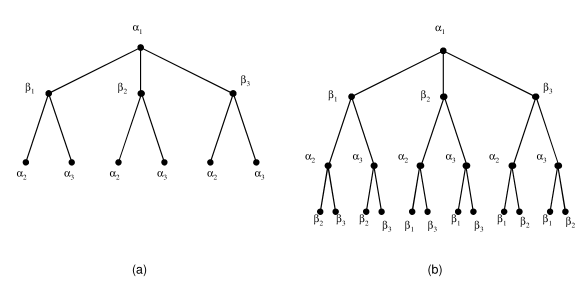
Figure 1: When $n=3$ (a) is $T_{\alpha_{i}}^{1}$ and (b) is $T_{\alpha_{i}}^{2}$.

A collection $\Lambda$ of edges in computation tree is called a T-matching if it no two edges of $\Lambda$ are adjacent in the tree ($\Lambda$ is a matching in the computation tree) and each non-leaf nodes are endpoint of exactly one edge from $\Lambda$. Let $t_{\alpha_{i}}^{k}(r)$ be the weight of maximum weight T-matching in $T_{\alpha_{i}}^{k}$ which uses the edge $(\alpha_{i},\beta_{r})$ at the root.

Now, we state two important lemmas that will lead to the proof of Theorem 1. The first lemma presents an important characterization of the min-sum algorithm while the second lemma relates the maximum weight T-matching of the computation tree and the MWM in $K_{n,n}$.

Lemma 1

At the end of the $k^{th}$ iteration of the min-sum algorithm, the belief at node $\alpha_{i}$ of $K_{n,n}$ is precisely $b_{\alpha_{i}}^{k}=[2t_{\alpha_{i}}^{k}(1)\ldots 2t_{\alpha_{i}}^{k}(n)]^{t}$.

Lemma 2

If $\pi^{*}$ is the MWM of graph $K_{n,n}$ then for $k>\frac{2nw^{*}}{\epsilon}$,

$$\pi^{*}(i)=\arg\max_{r}\{t_{\alpha_{i}}^{k}(r)\}.$$

That is, for $k$ large enough, the maximum weight T-matching in $T_{\alpha_{i}}^{k}$ chooses the edge $(\alpha_{i},\beta_{\pi^{*}(i)})$ at the root.

Proof:

Consider the min-sum algorithm. Let $b_{\alpha_{i}}^{k}=[b_{\alpha_{i}}^{k}(1),\ldots,b_{\alpha_{i}}^{k}(n)]^{t}$. Recall that $\pi^{k}=(\pi^{k}(i))$ where $\pi^{k}(i)=\arg\max_{r}\{b_{\alpha_{i}}^{k}(r)\}$. Then, by Lemmas 1 and 2, for $k>\frac{2nw^{*}}{\epsilon}$, $\pi^{k}=\pi^{*}$. ∎

Next, we present the proofs of Lemmas 1 and 2 in that order.

Proof:

It is known [20] that under the min-sum (or max-product) algorithm, the vector $b_{\alpha_{i}}^{k}$ corresponds to the correct max-marginals for the root $\alpha_{i}$ of the MAP assignment on the GM corresponding to $T_{\alpha_{i}}^{k}$. The pairwise compatibility functions force the MAP assignment on this tree to be a T-matching. Now, each edge has two endpoints and hence its weight is counted twice in the weight of T-matching.

Next consider the $j^{th}$ entry of $b_{\alpha_{i}}^{k}$, $b_{\alpha_{i}}^{k}(j)$. By definition, it corresponds to the MAP assignment with the value of $\alpha_{i}$ at the root being $j$. That is, $(\alpha_{i},\beta_{j})$ edge is chosen in the tree at the root. From the above discussion, $b_{\alpha_{i}}^{k}(j)$ must be equal to $2t_{\alpha_{i}}^{k}(j)$. ∎

Proof:

Assume the contrary that for some $k>\frac{2nw^{*}}{\epsilon}$,

$$\pi^{*}(i)\neq\arg\max_{r}t_{\alpha_{i}}^{k}(r)\stackrel{{\scriptstyle\triangle}}{{=}}\hat{i},~{}~{}\mbox{for some $i$}.$$ (11)

Then, let $\hat{i}=\pi^{*}(i_{1})$ for $i_{1}\neq i$. Let $\Lambda$ be the T-matching on $T_{\alpha_{i}}^{k}$ whose weight is $t_{\alpha_{i}}^{k}(\hat{i})$. We will modify $\Lambda$ and find $\Lambda^{\prime}$ whose weight is more than $\Lambda$ and which connects $(\alpha_{i},\beta_{\pi^{*}(i)})$ at the root instead of $(\alpha_{i},\beta_{\pi^{*}(i_{1})})$, thus contradicting with (11).

First note that the set of all edges of $T_{\alpha_{i}}^{k}$ whose projection in $K_{n,n}$ belong to $\pi^{*}$ is a T-matching which we denote by $\Pi^{*}$. Now consider paths $P_{\ell},~{}\ell\geq 0$ in $T_{\alpha_{i}}^{k}$, that contain edges from $\Pi^{*}$ and $\Lambda$ alternatively defined as follows. Let $\alpha_{0}=\mbox{root}~{}\alpha_{i}$, $i_{0}=i$ and $P_{1}=(\alpha_{0})$ be a single vertex path. Let $P_{2}=(\beta_{\pi^{*}(i_{0})},\alpha_{0},\beta_{\pi^{*}(i_{1})})$, where $i_{1}$ is such that $\alpha_{0}=\alpha_{i}$ is connected to $\beta_{\pi^{*}(i_{1})}$ under $\Lambda$. For $r\geq 1$, define $P_{2r+1}$ and $P_{2r+2}$ recursively as follows:

$$P_{2r+1}=(\alpha_{i_{-r}},P_{2r},\alpha_{i_{r}}),$$

$$P_{2r+2}=(\beta_{\pi^{*}(i_{-r})},P_{2r+1},\beta_{\pi^{*}(i_{r+1})})$$

where $\alpha_{i_{-r}}$ is the node at level $2r$ to which the endpoint node $\beta_{\pi^{*}(i_{-r+1})}$ of path $P_{2r}$ is connected to under $\Lambda$, and $i_{r+1}$ is such that $\alpha_{i_{r}}$ at level $2r$ (part of $P_{2r+1}$) is connected to $\beta_{\pi^{*}(i_{r+1})}$ under $\Lambda$. Note that, by definition, such paths $P_{\ell}$ for $\ell\leq k$ exist since the tree $T_{\alpha_{i}}^{k}$ has $k+1$ levels and can support a path of length at most $2k$ as defined above.

Example 2

The Figure 2(d) provides an example of such a path. The corresponding bipartite graph has $n=3$ with its MWM shown in figure 2(a). The Figure 2(d) shows $T^{5}_{\alpha_{1}}$, the computation tree for node $\alpha_{1}$, till level $k=5$. A path, $P_{5}$, is highlighted with thick edges alternatively complete and bold (edges from $\Lambda$) and dashed (edges from $\Pi^{*}$). In the figure, $P_{1}=(\alpha_{1})$; $P_{2}=(\beta_{1},\alpha_{1},\beta_{2})$; $P_{3}=(\alpha_{2},\beta_{1},\alpha_{1},\beta_{2},\alpha_{2})=(\alpha_{3},P_{2},\alpha_{2})$ and so on. Finally,

$$P_{5}=(\alpha_{1},\beta_{2},\alpha_{2},\beta_{1},\alpha_{1},\beta_{2},\alpha_{2},\beta_{3},\alpha_{3})=C_{1}\cup Q,$$

where $C_{1}=(\alpha_{1},\beta_{1},\alpha_{2},\beta_{2},\alpha_{1})$ is a cycle of length $4$ (see Figure 2(c)) and $Q=(\alpha_{1},\beta_{2},\alpha_{2},\beta_{3},\alpha_{3})$ is a path of length $4$ (see Figure 2(b)).

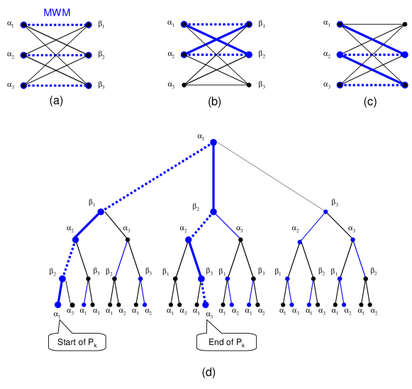
Figure 2: Consider a graph with MWM shown in (a). Projection of the path $P_{k}$ for $k=5$ as shown in (d) is decomposed to (b): path Q of length 4 and (c): cycle $C_{1}$ of length 4. The dashed edges belong to $\Pi^{*}$ while bold edges belong to $\Lambda$.

Now consider the path $P_{k}$ of length $2k$. Its edges are alternately from $\Lambda$ and $\pi^{*}$. Let us refer to the edges of $\Lambda$ as the $\Lambda$-edges of $P_{k}$. Replacing the $\Lambda$-edges of $P_{k}$ with their complement in $P_{k}$ produces a new matching $\Lambda^{\prime}$ in $T_{\alpha_{i}}^{k}$; this follows from the way the paths are constructed.

Lemma 3

The weight of T-matching $\Lambda^{\prime}$ is strictly higher than that of $\Lambda$ on tree $T_{\alpha_{i}}^{k}$.

This completes the proof of Lemma 2 since Lemma 3 shows that $\Lambda$ is not the maximum weight T-matching on $T_{\alpha_{i}}^{k}$, leading to a contradiction. ∎

Now, we provide the proof of Lemma 3.

Proof:

It suffices to show that the total weight of the $\Lambda$-edges is less than the total weight of their complement in $P_{k}$. Consider the projection $P^{\prime}_{k}$ of $P_{k}$ in the graph $K_{n,n}$. $P^{\prime}_{k}$ can be decomposed into a union of a set of simple cycles $\{C_{1},C_{2},\ldots,C_{m}\}$ and at most one even length path $Q$ of length at most $2n$. Since each simple cycle has at most $2n$ vertices and the length of $P_{k}$ is $2k$,

$$m\geq\frac{2k}{2n}=\frac{k}{n}.$$ (12)

Consider one of these simple cycles, say $C_{s}$. Construct the matching $\pi^{\prime}$ in $K_{n,n}$ as follows: (i) For $\alpha_{l}\in C_{s}$, select edges incident on $\alpha_{l}$ that belong to $\Lambda$. Such edges exist by the property of the path $P_{k}$ that contains $C_{s}$. (ii) For $\alpha_{l}\notin C_{s}$, connect it according to $\pi^{*}$, that is, add the edge $(\alpha_{l},\beta_{\pi^{*}(l)})$.

Now $\pi^{\prime}\neq\pi^{*}$ by construction. Since the MWM is unique, the definition of $\epsilon$ gives us

$$W_{\pi^{\prime}}\leq W_{\pi^{*}}-\epsilon.$$

But, $W_{\pi^{*}}-W_{\pi^{\prime}}$ is exactly equal to the total weight of the $\Pi^{*}$-edges of $C_{s}$ minus the total weight of the $\Lambda$-edges of $C_{s}$. Thus,

$$\textrm{\small weight of $\Lambda$-edges of $C_{s}$}-\textrm{\small weight of $\Pi^{*}$-edges of $C_{s}$} = -(W_{\pi^{*}}-W_{\pi^{\prime}})~{}~{}\leq~{}~{}-\epsilon.$$ (13)

Since the path $Q$ is of even length, either the first edge or the last edge is an $\Lambda$-edge. Without loss of generality, assume it is the last edge. Then, let

$$Q=(\beta_{\pi^{*}(i_{j_{1}})},\alpha_{i_{j_{1}}},\beta_{\pi^{*}(i_{j_{2}})},\ldots,\beta_{\pi^{*}(i_{j_{l}})},\alpha_{i_{j_{l}}},\beta_{\pi^{*}(i_{j_{l+1}})}).$$

Now consider the cycle

$$C=(\beta_{\pi^{*}(i_{j_{1}})},\alpha_{i_{j_{1}}},\beta_{\pi^{*}(i_{j_{2}})},\ldots,\beta_{\pi^{*}(i_{j_{l}})},\alpha_{i_{j_{l}}},\beta_{\pi^{*}(i_{j_{1}})}).$$

Alternate edges of $C$ are from the maximum weight matching $\pi^{*}$. Hence, using the same argument as above, we obtain

$$\textrm{\small weight of $\Lambda$-edges of $Q$}-\textrm{\small weight of $\Pi^{*}$-edges of $Q$} = \sum_{1\leq r\leq l}w_{i_{j_{r}}\pi^{*}(i_{j_{r+1}})}-\sum_{1\leq r\leq l}w_{i_{j_{r}}\pi^{*}(i_{j_{r}})}$$ (14)

$$\leq -\epsilon+|w_{i_{j_{l}}\pi^{*}(i_{j_{1}})}|+|w_{i_{j_{l}}\pi^{*}(i_{j_{l+1}})}|$$

$$\leq -\epsilon+2w^{*}.$$

From (12)-(14), we obtain that for T-matchings $\Lambda^{\prime}$ and $\Lambda$ in $T_{\alpha_{i}}^{k}$:

$$\textrm{\small weight of $\Lambda$}-\textrm{\small weight of $\Lambda^{\prime}$} \leq -(m+1)(\epsilon)+2w^{*}$$ (15)

$$\leq -\frac{k}{n}\epsilon+2w^{*}$$

$$< 0.$$

This completes the proof of Lemma 3. ∎

IV Complexity

In this section, we will analyze the complexity of the min-sum algorithm described in Section II-C. Theorem 1 suggests that the number of iterations required to find MWM is $O\left(\frac{nw^{*}}{\epsilon}\right)$. Now, in each iteration of Min-Sum algorithm each node sends a vector of size $n$ (i.e. $n$ numbers) to each of the $n$ nodes in the other partition. Thus, total number of messages exchanged in each iteration are $O(n^{2})$ with each message of length $n$. Now, each node performs $O(n)$ basic computational operations (comparison, addition) to compute each element in a message vector of size $n$. That is, each node performs $O(n^{2})$ computational operations to compute a message vector in each iteration. Since each node sends $n$ message vectors, the total cost is $O(n^{3})$ per node or $O(n^{4})$ per iteration for all nodes. Thus, total cost for $O(nw^{*}/\epsilon)$ iterations is $O(n^{5}w^{*}/\epsilon)$.

Thus, for fixed $w^{*}$ and $\epsilon$, the running time of algorithm scales as $O(n^{5})$. The known algorithms such as Edmond-Karp’s algorithm [8] or Auction algorithm [6] have complexity of $O(n^{3})$. In what follows, we simplify the Min-Sum algorithm so that overall running time of the algorithm becomes $O(n^{3})$ for fixed $w^{*}$ and $\epsilon$. We make a note here that Edmond-Karp’s algorithm is strongly polynomial (i.e. does not depend on $w^{*}$ and $\epsilon$) while Auction algorithm’s complexity is $O(n^{3}w^{*}/\epsilon)$.

IV-A SIMPLIFIED MIN-SUM ALGORITHM FOR $K_{n,n}$

We first present the algorithm and show that it is exactly the same as Min-Sum algorithm. Later, we analyze the complexity of the algorithm.

Simplified Min-Sum Algorithm.  

• Unlike Min-Sum algorithm, now each $\alpha_{i}$ sends a number to $\beta_{j}$ and vice-versa. Let the message from $\alpha_{i}$ to $\beta_{j}$ in iteration $k$ be denoted as

  $$\hat{m}^{k}_{\alpha_{i}\rightarrow\beta_{j}}$$

  Similarly, the messages from $\beta_{j}$ to $\alpha_{i}$ in iteration $k$ be denoted as

  $$\hat{m}^{k}_{\beta_{j}\rightarrow\alpha_{i}}$$

• Initially $k=0$ and set the messages as follows.

  $$\hat{m}_{\alpha_{i}\rightarrow\beta_{j}}^{0}=w_{ij}$$

  Similarly,

  $$\hat{m}^{0}_{\beta_{j}\rightarrow\alpha_{i}}=w_{ij}$$

• For $k\geq 1$, messages in iteration $k$ are obtained from messages of iteration $k-1$ recursively as follows:

  $$\hat{m}_{\alpha_{i}\rightarrow\beta_{j}}^{k} = w_{ij}-\max_{\ell\neq j}\hat{m}_{\beta_{\ell}\rightarrow\alpha_{i}}^{k-1},$$

  $$\hat{m}_{\beta_{j}\rightarrow\alpha_{i}}^{k} = w_{ij}-\max_{\ell\neq i}\hat{m}_{\alpha_{\ell}\rightarrow\beta_{j}}^{k-1}$$ (16)

• The estimated MWM at the end of iteration $k$ is $\pi^{k}$, where $\pi^{k}(i)=\arg\max_{1\leq j\leq n}\{\hat{m}_{\beta_{j}\rightarrow\alpha_{i}}^{k}\},$ for $1\leq i\leq n$.

• Repeat (3)-(4) till $\pi^{k}$ converges.

 

Now, we state and prove the claim that relates the above modified algorithm to the original Min-Sum algorithm.

Lemma 4

In Min-Sum algorithm adding an equal amount to all coordinates of any message vector $M_{\alpha_{i}\rightarrow\beta_{j}}^{k}$ (similarly $M_{\beta_{j}\rightarrow\alpha_{i}}^{k}$) at anytime does not change the resulting estimated matching $\pi^{m}$ for all $k,m$.

Proof:

If a number is added to all coordinates of $M_{\alpha_{i}\rightarrow\beta_{j}}^{k}$ it is not hard to see from equation (9) and structure of $\psi_{\alpha_{i}\beta_{j}}(\cdot,\cdot)$ that other message and belief vectors will change only up to an additive constant to their coordinates. Hence these changes do not affect $\pi^{m}(i)=\arg\max_{1\leq j\leq n}\{b_{\alpha_{i}}^{m}(j)\},$ for $1\leq i\leq n$. ∎

Lemma 5

The algorithms Min-Sum and Simplified Min-Sum produce identical estimated matchings $\pi^{m}$ at the end of every iteration $m$.

Proof:

Consider the Min-Sum algorithm. In particular, consider a message vector $M_{\alpha_{i}\rightarrow\beta_{j}}^{k}$ in iteration $k$. First, we claim that all for any given $k\geq 0$, $m_{\alpha_{i}\rightarrow\beta_{j}}^{k}(r),r\neq i$ are the same. That is, for $r_{1}\neq r_{2}$ and $r_{1},r_{2}\neq i$,

$$m_{\alpha_{i}\rightarrow\beta_{j}}^{k}(r_{1})=m_{\alpha_{i}\rightarrow\beta_{j}}^{k}(r_{2}).$$

For $k=0$, this claim holds by definition. For $k\geq 1$, consider the definition of $m_{\alpha_{i}\rightarrow\beta_{j}}^{k}(r),r\neq i$.

$$m_{\alpha_{i}\rightarrow\beta_{j}}^{k}(r)=\max_{1\leq q\leq n}\psi_{\alpha_{i}\beta_{j}}(q,r)\left[w_{iq}+\sum_{\ell\neq j}m_{\beta_{\ell}\alpha_{i}}^{k-1}(q)\right]=\max_{q\neq j}\left[w_{iq}+\sum_{\ell\neq j}m_{\beta_{\ell}\alpha_{i}}^{k-1}(q)\right].$$ (17)

The first equality follows from definition in Min-Sum algorithm while second equality follows from property of $\psi_{\alpha_{i}\beta_{j}}(\cdot,\cdot)$. The equation (17) is independent of $r(\neq i)$. This proves the desired claim.

The above stated property of Min-Sum algorithm immediately implies that the vector $M_{\alpha_{i}\rightarrow\beta_{j}}^{k}$ has only two distinct values, one corresponding to $m_{\alpha_{i}\rightarrow\beta_{j}}^{k}(i)$ and the other corresponding to $m_{\alpha_{i}\rightarrow\beta_{j}}^{k}(r),r\neq i$. Now subtract $m_{\alpha_{i}\rightarrow\beta_{j}}^{k}(r),r\neq i$ from all coordinates of $M_{\alpha_{i}\rightarrow\beta_{j}}^{k}$. Lemma 4 guarantees the resulting matching $\pi^{m}$ for all $m$ does not change. Performing the same modification to all message vectors yields a Modified Min-Sum algorithm with the same outcome as Min-Sum. But each message vector $M_{\alpha_{i}\rightarrow\beta_{j}}^{k}$ in this Modified Min-Sum has all coordinates equal to zero except the $i^{th}$ coordinate. Denote these $i^{th}$ coordinates by $\tilde{m}_{\alpha_{i}\rightarrow\beta_{j}}^{k}$. Now equation (9) shows these for all $i,j,k$ numbers $\tilde{m}_{\alpha_{i}\rightarrow\beta_{j}}^{k}$ satisfy the following recursive equations:

$$\tilde{m}_{\alpha_{i}\rightarrow\beta_{j}}^{k} = w_{ij}-\max_{\ell\neq j}(\tilde{m}_{\beta_{\ell}\rightarrow\alpha_{i}}^{k-1}+w_{i\ell}),$$

$$\tilde{m}_{\beta_{j}\rightarrow\alpha_{i}}^{k} = w_{ij}-\max_{\ell\neq i}(\tilde{m}_{\alpha_{\ell}\rightarrow\beta_{j}}^{k-1}+w_{\ell j})$$ (18)

Similarly for new beliefs we have:

$$\tilde{b}_{\alpha_{i}}^{k}(r) = \tilde{m}_{\beta_{r}\rightarrow\alpha_{i}}^{k}+w_{ir},$$

$$\tilde{b}_{\beta_{j}}^{k}(s) = \tilde{m}_{\alpha_{s}\rightarrow\beta_{j}}^{k}+w_{sj}$$ (19)

Now by adding $w_{ij}$ to each side of (18) and dividing them by $2$ it can be seen from (16) that numbers $\frac{\tilde{m}_{\alpha_{i}\rightarrow\beta_{j}}^{k}+w_{ij}}{2}$ and $\hat{m}_{\alpha_{i}\rightarrow\beta_{j}}^{k}$ satisfy the same recursive equations. They also satisfy the same initial conditions. As result for all $i,j,k$ we have

$$\hat{m}_{\alpha_{i}\rightarrow\beta_{j}}^{k}=\frac{\tilde{m}_{\alpha_{i}\rightarrow\beta_{j}}^{k}+w_{ij}}{2}=\tilde{b}_{\alpha_{i}}(j)$$ (20)

and

$$\hat{m}_{\beta_{j}\rightarrow\alpha_{i}}^{k}=\frac{\tilde{m}_{\beta_{j}\rightarrow\alpha_{i}}^{k}+w_{ij}}{2}=\tilde{b}_{\beta_{j}}(i)$$ (21)

This shows that the estimated matching computed at nodes in Modified Min-Sum and Simplified Min-Sum algorithms are exactly the same at each iteration which completes the proof of Lemma 5. ∎

Note 5. The simplified min-sum equations can also be derived in a direct way by looking interpretation of the messages $\{\hat{m}_{\alpha_{i}\to\beta_{j}}^{k}\}_{i,j,k}$ in the computation tree. More specifically consider the level-$(k+1)$ computation tree rooted at $\alpha_{i}$, $T_{\alpha_{i}}^{k+1}$. Also consider its subtree, $T_{\alpha_{i},\beta_{j}}^{k}$ , that is built by adding the edge $(\alpha_{i},\beta_{j})$ at the root of $T_{\alpha_{i}}^{k+1}$ to graph of all descendants of $\beta_{j}$. One can show that the message $\hat{m}_{\beta_{j}\to\alpha_{i}}^{k}$ is equal to the difference between weight of maximum weight $T$-matching in $T_{\alpha_{i},\beta_{j}}^{k}$ that uses the edge $(\alpha_{i},\beta_{j})$ at the root and weight of the maximum weight $T$-matching in $T_{\alpha_{i},\beta_{j}}^{k}$ that does not use that edge. Now a simple induction gives us the update equations (16).

IV-B COMPLEXITY OF SIMPLIFIED MIN-SUM

The Lemma 5 and Theorem 1 immediately imply that the Simplified Min-Sum, like Min-Sum, converges after $O\left(\frac{nw^{*}}{\epsilon}\right)$ iterations. As described above, the Simplified Min-Sum algorithm requires total $O(n^{2})$ messages per iteration. Thus, for fixed $w^{*}$ and $\epsilon$ the algorithm requires total $O(n^{3})$ messages to be exchanged.

Now, we consider the number of computational operations done by each node in an iteration. From the description of Simplified Min-Sum algorithm, it may seem that each node will require to do $O(n)$ work for sending each message and thus $O(n^{2})$ work overall at one node. But, we present a simple method that shows each node can compute message for all of its $n$ neighbors with $O(n)$ computational operation (comparison, addition/subtraction). This will result in $O(n^{2})$ overall computation per iteration. Thus, it will take $O\left(\frac{n^{3}w^{*}}{\epsilon}\right)$ computation in $O\left(\frac{nw^{*}}{\epsilon}\right)$ iterations. This will result in total complexity of $O\left(\frac{n^{3}w^{*}}{\epsilon}\right)$ in terms of overall messages as well as computation operations.

Here we describe an algorithm to compute messages $\hat{m}^{k}_{\alpha_{1}\rightarrow\beta_{j}},1\leq j\leq n$ using received messages $\hat{m}^{k-1}_{\beta_{j}\rightarrow\alpha_{1}},1\leq j\leq n$. This is the same algorithm that all $\alpha_{i},1\leq i\leq n,$ and $\beta_{j},1\leq j\leq n$, need to employ. Now, define

$$i_{1} = \textrm{argmax}_{1\leq j\leq n}\hat{m}^{k-1}_{\beta_{j}\rightarrow\alpha_{1}}$$

$$i_{2} = \textrm{argmax}_{1\leq j\leq n,j\neq i_{1}}\hat{m}^{k-1}_{\beta_{j}\rightarrow\alpha_{1}}$$

$$\mbox{Mx}_{1} = \hat{m}^{k-1}_{\beta_{i_{1}}\rightarrow\alpha_{1}}$$

$$\mbox{Mx}_{2} = \hat{m}^{k-1}_{\beta_{i_{2}}\rightarrow\alpha_{1}}$$

Then, from (16) we obtain

$$\hat{m}^{k}_{\alpha_{1}\rightarrow\beta_{i_{1}}} = w_{1i_{1}}-\mbox{Mx}_{2},$$

$$\hat{m}^{k}_{\alpha_{1}\rightarrow\beta_{j}} = w_{1j}-\mbox{Mx}_{1}\quad\textrm{for $j\neq i_{1}$}.$$ (22)

We see that computing all messages $\hat{m}^{k}_{\alpha_{1}\rightarrow\beta_{j}}$ takes $O(n)$ operations. From (22), it takes node $\alpha_{1}$ $O(n)$ computations to find $i_{1},i_{2},\mbox{Mx}_{1},\mbox{Mx}_{2}$, then it takes $O(1)$ computation to compute each of the $\hat{m}^{k}_{\alpha_{1}\rightarrow\beta_{j}},1\leq j\leq n$. That is, total $O(n)$ operations for computing all messages $\hat{m}^{k}_{\alpha_{1}\rightarrow\beta_{j}},1\leq j\leq n$.

Thus, we have established that each node $\alpha_{i},1\leq i\leq n,$ and $\beta_{j},1\leq j\leq n,$ need to perform $O(n)$ computation to compute all of its messages in a given iteration. That is, the total computation cost per iteration is $O(n^{2})$. In summary, Theorem 1, Lemma 5 and discussion of this Section IV-B immediately yield the following result.

Theorem 2

The Simplified Min-Sum algorithm finds the Maximum Weight Matching in $O\left(\frac{nw^{*}}{\epsilon}\right)$ iterations with total computation cost of $O\left(\frac{n^{3}w^{*}}{\epsilon}\right)$ and $O\left(\frac{n^{3}w^{*}}{\epsilon}\right)$ total number of message exchanges.

V AUCTION AND MIN-SUM

In this section, we will first recall the auction algorithm [6] and then describe its relation to the min-sum algorithm.

V-A AUCTION ALGORITHM FOR MWM

The Auction algorithm finds the MWM via an “auction”: all $\alpha_{i}$ become buyers and all $\beta_{j}$ become objects. Let $p_{j}$ denote the price of $\beta_{j}$ and $w_{ij}$ be the value of object $\beta_{j}$ for buyer $\alpha_{i}$. The net benefit of an assignment or matching $\pi$ is defined as

$$\sum_{i=1}^{n}\left(w_{i\pi(i)}-p_{\pi(i)}\right).$$

The goal is to find $\pi^{*}$ that maximizes this net benefit. It is clear that for any set of prices $p_{1},\ldots,p_{n}$, the MWM maximizes the net benefit. The auction algorithm is an iterative method for finding the optimal prices and an assignment that maximizes the net benefit (and is therefore the MWM).

Auction Algorithm.

 

• Initialize the assignment $S=\emptyset$, the set of unassigned buyers $I=\{\alpha_{1},\ldots,\alpha_{n}\}$, and prices $p_{j}=0$ for all $j$.

• The algorithm runs in two phases, which are repeated until $S$ is a complete matching.

• Phase 1: Bidding.
  For all $\alpha_{i}\in I$,

  • Find benefit maximizing $\beta_{j}$. Let,

    $$j_{i}=\textrm{argmax}_{j}\{w_{ij}-p_{j}\},~{}v_{i}=\max_{j}\{w_{ij}-p_{j}\},~{}\mbox{and}~{}u_{i}=\max_{j\neq j_{i}}\{w_{ij}-p_{j}\}.$$ (23)

  • Compute the ”bid” of buyer $\alpha_{i}$, denoted by $b_{\alpha_{i}\to\beta_{j_{i}}}$ as follows: given a fixed positive constant $\delta$,

    $$b_{\alpha_{i}\rightarrow\beta_{j_{i}}}=w_{ij_{i}}-u_{i}+\delta.$$

• Phase 2: Assignment.
  For each object $\beta_{j}$,

  • Let $P(j)$ be the set of buyers from which $\beta_{j}$ received a bid. If $P(j)\neq\emptyset$, increase $p_{j}$ to the highest bid,

    $$p_{j}=\max_{\alpha_{i}\in P(j)}b_{\alpha_{i}\rightarrow\beta_{j}}.$$

  • Remove the maximum bidder $\alpha_{i_{j}}$ from $I$ and add $(\alpha_{i_{j}},\beta_{j})$ to $S$. If $(\alpha_{k},\beta_{j})\in S,~{}k\neq i_{j}$, then put $\alpha_{k}$ back in $I$.

 

Theorem 3 ([5])

If $0<\delta<\epsilon/n$, then the assignment $S$ converges to the MWM in $O(nw^{*}/\epsilon)$ iterations with running time $O(n^{3}w^{*}/\epsilon)$ (where $\epsilon$ and $w^{*}$ are as defined earlier).

V-B CONNECTING MIN-SUM AND AUCTION

The similarity between equations (22) and (23) suggests a connection between the min-sum and auction algorithms. Next, we describe modifications to the min-sum and auction algorithms, called min-sum auction I and min-sum auction II, respectively. We will show that these versions are equivalent and derive some of their key properties. Here we consider the naïve auction algorithm (when $\delta=0$) and deal with the case $\delta>0$ in the next section.

Min-Sum Auction I

 

• Each $\alpha_{i}$ sends a number to $\beta_{j}$ and vice-versa. Let the messages in iteration $k$ be denoted as $\tilde{m}^{k}_{\alpha_{i}\rightarrow\beta_{j}},\ \tilde{m}^{k}_{\beta_{j}\rightarrow\alpha_{i}}\in\mathbb{R}$.

• Initialize $k=0$ and set $\tilde{m}_{\beta_{j}\rightarrow\alpha_{i}}^{0}=0$.

• For $k\geq 1$, update messages as follows:

  $$\tilde{m}_{\alpha_{i}\rightarrow\beta_{j}}^{k} = w_{ij}-\max_{\ell\neq j}\{w_{i\ell}-\tilde{m}_{\beta_{\ell}\rightarrow\alpha_{i}}^{k-1}\},$$

  $$\tilde{m}_{\beta_{j}\rightarrow\alpha_{i}}^{k} = \max_{\ell=1}^{n}\ \tilde{m}_{\alpha_{\ell}\rightarrow\beta_{j}}^{k},$$ (24)

• The estimated MWM at the end of iteration $k$ is the set of edges

  $$\pi^{k}=\{(\alpha_{i_{j}},\beta_{j})|\ i_{j}=\arg\max_{1\leq\ell\leq n}\{\tilde{m}_{\alpha_{\ell}\rightarrow\beta_{j}}^{k}\}\ 1\leq j\leq n,\textrm{ and }\tilde{m}_{\alpha_{i_{j}}\rightarrow\beta_{j}}^{k}\geq\tilde{m}_{\beta_{j}\rightarrow\alpha_{i}}^{k-1}\}$$

• Repeat (3)-(4) till $\pi^{k}$ is a complete matching.

 

Min-Sum Auction II.

 

• Initialize the assignment $S=\emptyset$ and prices $p_{j}=0$ for all $j$.

• The algorithm runs in two phases, which are repeated until $S$ is a complete matching.

• Phase 1: Bidding.
  For all $\alpha_{i}$,

  • Find $\beta_{j}$ that maximizes the benefit. Let,

    $$j_{i}=\textrm{argmax}_{j}\{w_{ij}-p_{j}\},~{}v_{i}=\max_{j}\{w_{ij}-p_{j}\},~{}\mbox{and}~{}u_{i}=\max_{j\neq j_{i}}\{w_{ij}-p_{j}\}.$$ (25)

  • Compute the ”bid” of buyer $\alpha_{i}$, denoted by $b_{\alpha_{i}\to\beta_{j}}$:

    $$b_{\alpha_{i}\rightarrow\beta_{j_{i}}}=w_{ij_{i}}-u_{i},~{}\mbox{and}~{}b_{\alpha_{i}\to\beta_{j}}=w_{ij}-v_{i},~{}j\neq j_{i}.$$

• Phase 2: Assignment.
  For each object $\beta_{j}$,

  • Set price $p_{j}$ to the highest bid, $p_{j}=\max_{\alpha_{i}}b_{\alpha_{i}\rightarrow\beta_{j}}.$

  • Reset $S=\emptyset$. Then, for each $j$ add the pair $(\alpha_{i_{j}},\beta_{j})$ to $S$ if $b_{\alpha_{j_{i}}\rightarrow\beta_{j}}\geq p_{j}$, where $\alpha_{i_{j}}$ is a buyer attaining the maximum in step (3).

 

Theorem 4

The algorithms min-sum auction I and II are equivalent.

Proof:

Let $b^{k}_{\alpha_{i}\to\beta_{j}}$ and $p^{k}_{j}$ denote the bids and prices at the end of iteration $k$ in algorithm min-sum auction II. Now, identify $b^{k}_{\alpha_{i}\to\beta_{j}}$ with $\tilde{m}^{k}_{\alpha_{i}\to\beta_{j}}$ and $p^{k}_{j}$ with $\tilde{m}^{k}_{\beta_{j}\to\alpha_{i}}$. Then it is immediate that min-sum auction II becomes identical to min-sum auction I. This completes the proof of Theorem 4. ∎

Next we will prove that if the min-sum auction algorithm terminates (we omit reference to I or II), it finds the correct maximum weight matching. As we will see, the proof uses standard arguments (see [6] for example).

Theorem 5

Let $\sigma$ be the termination matching of the min-sum auction I (or II). Then it is the MWM, i.e. $\sigma=\pi^{*}$.

Proof:

The proof follows by establishing that at termination, the messages of min-sum auction form the optimal solution for the dual of the MWM problem and $\sigma$ is the corresponding optimal solution to the primal, i.e. MWM. To do so, we first state the dual of the MWM problem

$$\min \sum_{i=1}^{n}r_{i}+\sum_{j=1}^{n}p_{j}$$

subject to $$r_{i}+p_{j}~{}\geq~{}w_{ij}.$$ (26)

Let $(r^{*},p^{*})$ be the optimal solution to the above stated dual problem and let $\pi^{*}$ solve the primal MWM problem. Then, the standard complimentary slackness conditions are:

$$r^{*}_{i}+p^{*}_{\pi^{*}(i)} = w_{i\pi^{*}(i)}.$$ (27)

Thus, $(r^{*},p^{*},\pi^{*})$ are the optimal dual-primal solution for the MWM problem if and only if (a) $\pi^{*}$ is a matching, (b) $(r^{*},p^{*})$ satisfy (26), and (c) the triple satisfies (27). To complete the proof we will prove the existence of $r^{*},p^{*}$ such that $(r^{*},p^{*},\sigma)$ satisfy (a), (b) and (c).

To this end, first note that $\sigma$ is a matching by the termination condition of the algorithm; thus, condition (a)is satisfied. We’ll consider the min-sum auction II algorithm for the purpose of the proof. Suppose the algorithm terminates at some iteration $k$. Let $p^{k-1}_{j}$ and $p^{k}_{j}$ be the prices of $\beta_{j}$ in iterations $k-1$ and $k$ respectively. Since all $\beta_{j}$s are matched at the termination, from step (4) of the min-sum auction II, we obtain

$$p^{k}_{j} \geq p^{k-1}_{j},~{}~{}\forall j.$$ (28)

At termination (iteration $k$), $\alpha_{i}$ is matched with $\beta_{\sigma(i)}$ or $\beta_{j}$ is matched with $\alpha_{\sigma^{-1}(j)}$. By the definition of the min-sum auction II algorithm,

$$p^{k}_{j} = w_{\sigma^{-1}(j)j}-\max_{\ell\neq j}\left[w_{\sigma^{-1}(j)\ell}-p^{k-1}_{\ell}\right].$$ (29)

From (28) and (29), we obtain that

$$w_{\sigma^{-1}(j)j}-p^{k}_{j} \geq \max_{\ell\neq j}\left[w_{\sigma^{-1}(j)\ell}-p^{k}_{\ell}\right].$$ (30)

Define, $r^{*}_{i}=w_{i\sigma(i)}-p^{k}_{\sigma(i)}$ and $p^{*}_{j}=p^{k}_{j}$. Then, from (30) $(r^{*},p^{*})$ satisfy the dual feasibility, that is (26). Further, by definition they satisfy the complimentary slackness condition (27). Thus, the triple $(r^{*},p^{*},\sigma)$ satisfies (a), (b) and (c) as required. Hence, the algorithm min-sum auction II produces the MWM, i.e. $\sigma=\pi^{*}$. ∎

The min-sum auction II algorithm looks very similar to the auction algorithm and inherits some of its properties. However, it also inherits some properties of the min-sum algorithm. This causes it to behave differently from the auction algorithm. The proof of convergence of auction algorithm relies on two properties of the auctioning mechanism: (a) the prices are always non-decreasing and (b) the number of matched objects is always non-decreasing. By design, (a) and (b) can be shown to hold for the auction algorithm. However, it is not clear if (a) and (b) are true for min-sum auction. In what follows, we state the result that prices are eventually non-decreasing in the min-sum auction algorithm; however it seems difficult to establish a statement similar to (b) for the min-sum algorithm as of now.

Theorem 6

If $\pi^{*}$ is unique then in the min-sum auction II algorithm, prices eventually increase. That is, $\forall k\in\mathbb{Z}^{+};~{}\exists~{}T>k~{}s.t.~{}\forall t\geq T;~{}p_{j}^{t}>p_{j}^{k},~{}1\leq j\leq n$

Proof:

Proof of Theorem (6) is essentially based on (i) the equivalence between the min-sum auction algorithms I and II, and (ii) arguments very similar to the ones used in the proof of Lemma 2 , where we relate prices with the computation tree. ∎

Our simulations suggests that in the absence of the condition “$\tilde{m}_{\alpha_{i_{j}}\rightarrow\beta_{j}}^{k}\geq\tilde{m}_{\beta_{j}\rightarrow\alpha_{i}}^{k-1}$” from step (4) of min-sum auction I, the algorithm always terminates and finds the MWM as long as it is unique. This along with Theorem 6 leads us to the following conjecture.

Conjecture 1

If $\pi^{*}$ is unique then the min-sum auction I terminates in a finite number of iterations if condition “$\tilde{m}_{\alpha_{i_{j}}\rightarrow\beta_{j}}^{k}\geq\tilde{m}_{\beta_{j}\rightarrow\alpha_{i}}^{k-1}$” is removed from step (4).

V-C RELATION TO $\delta$-RELAXATION

In the previous section, we established a relation between the min-sum and auction (with $\delta=0$) algorithms. In [6, 5] the author extends the auction algorithm to obtain guaranteed convergence in a finite number of iterations via a $\delta$-relaxation for some $\delta>0$. At termination the $\delta$-relaxed algorithm produces a triple $(r^{*},p^{*},\pi^{*})$ such that (a1) $\pi^{*}$ is a matching, (b1) $(r^{*},p^{*})$ satisfy (26) and (c1) the following modified complimentary slackness conditions are satisfied:

$$r^{*}_{i}+p^{*}_{\pi^{*}(i)} \leq w_{i\pi^{*}(i)}+\delta.$$ (31)

The conditions (c1) are referred to as $\delta$-CS conditions in [6]. This modification is reflected in the description of the auction algorithm where we have added $\delta$ to each bid in step (2). We established the relation between min-sum and auction for $\delta=0$ in the previous section. Here we make a note that for every $\delta>0$, the similar relation holds. To see this, we consider min-sum auction I and II where the bid computation is modified as follows: modify step (3) of min-sum auction I as $\tilde{m}^{k}_{\alpha_{i}\to\beta_{j}}=w_{ij}-\max_{\ell\neq j}\{w_{i\ell}-\tilde{m}_{\beta_{\ell}\rightarrow\alpha_{i}}^{k-1}\}+\delta,$ and modify step (2) of min-sum auction II as $b_{\alpha_{i}\rightarrow\beta_{j_{i}}}=w_{ij_{i}}-u_{i}+\delta,~{}\mbox{and}~{}b_{\alpha_{i}\to\beta_{j}}=w_{ij}-v_{i}+\delta,~{}j\neq j_{i}.$ For these modified algorithms, we obtain the following result using arguments very similar to the ones used in Theorem 5.

Theorem 7

For $\delta>0$, let $\sigma$ be the matching obtained from the modified min-sum auction algorithm I (or II). Then, $w_{\sigma}\geq w_{\pi^{*}}-n\delta$ (i.e. $\sigma$ is within $n\delta$ of the MWM).

VI DISCUSSION AND CONCLUSION

In this paper, we proved that the max-product algorithm converges to the desirable fixed point in the context of finding the MWM for a bipartite graph, even in the presence of loops. This result has a twofold impact. First, it will possibly open avenues for a demystification of the max-product algorithm. Second, the same approach may provably work for other combinatorial optimization problems and possibly lead to better algorithms.

Using the regularity of the structure of the problem, we managed to simplify the max-product algorithm. In the simplified algorithm each node needs to perform $O(n)$ addition-subtraction operations in each iteration. Since $O(n)$ iterations are required in the worst case, for finite $w^{*}$ and $\epsilon$, the algorithm requires $O(n^{3})$ operations at the most. This is comparable with the best known MWM algorithm. Furthermore, the distributed nature of the max-product algorithm makes it particularly suitable for networking applications like switch scheduling where scalability is a necessary property.

Future work will consist of trying to extend our result to finding the MWM in a general graph, as our current arguments do not carry over. Also, we would like to obtain tighter bounds on the running time of the algorithm since simulation studies show that the algorithm runs much faster on average than the worst case bound obtained in this paper.

References

- [1] S. M. Aji, G. B. Horn and R. J. McEliece, “On the Convergence of Iterative Decoding on Graphs with a Single Cycle,” in Proc. IEEE Int. Symp. Information Theory, 1998, p. 276.
- [2] S. M. Aji and R. J. McEliece, “The Generalized Distributive Law,” IEEE Trans. Inform. Theory, Vol. 46, pp. 325-343, 2000.
- [3] M. Bayati, D. Shah and M. Sharma, “Max Weight Matching via Max Product Belief Propagation,” IEEE ISIT, 2005.
- [4] M. Bayati, D. Shah and M. Sharma, “A simpler max-product maximum weight matching algorithm and the auction algorithm,” IEEE ISIT, 2006.
- [5] D. P. Bertsekas, “Auction Algorithms for Network Flow Problems: A Tutorial Introduction,” Computational Optimization and Applications, Vol. 1, pp. 7-66, 1992
- [6] D. Bertsekas and J. Tsitsiklis, “Parallel and Distributed Computation: Numerical Methods,” Englewood Cliffs NJ: Prentice Hall, 1989.
- [7] R. G. Gallager, “Low Density Parity Check Codes,” Cambridge, MA: MIT Press, 1963.
- [8] J. Edmonds and R. Karp, “Theoretical Improvements in Algorithmic Efficiency for Network Flow Problems,” Jour. of the ACM, Vol. 19, pp 248-264, 1972.
- [9] B.J. Frey, R. Koetter, “Exact inference using the attenuated max-product algorithm”, Advanced Mean Field Methods: Theory and Practice, ed. Manfred Opper and David Saad, MIT Press, 2000.
- [10] G. B. Horn, “Iterative Decoding and Pseudocodewords,” Ph.D. dissertation, Department of Electrical Engineering, CalTech, Pasadena, CA, 1999.
- [11] S. Lauritzen, “Graphical models,” Oxford University Press, 1996.
- [12] E. Lawler, “Combinatorial Optimization: Networks and Matroids”, Holt, Rinehart and Winston, New York, 1976.
- [13] N. McKeown, V. Anantharam and J. Walrand, “Achieving 100 % Throughput in an Input-Queued Switch,” Infocom, Vol. 1, pp 296-302, 1996.
- [14] M. Mezard, G. Parisi and R. Zecchina “Analytic and algorithmic solution of random satisfiability problems,” Science, 297,812, 2002.
- [15] J. Pearl, “Probabilistic Reasoning in Intelligent Systems: Networks of Plausible Inference,” San Francisco, CA: Morgan Kaufmann, 1988.
- [16] T. Richardson and R. Urbanke, “The Capacity of Low-Density Parity Check Codes under Message-Passing Decoding,” IEEE Trans. Info. Theory, Vol. 47, pp 599-618, 2001.
- [17] M. Wainwright, M. Jordan, “Graphical models, exponential families, and variational inference,” Dept. of Stat., University of Cal., Berkeley, CA, Tech. Report, 2003.
- [18] M. J. Wainwright, T. S. Jaakkola, and A. S. Willsky, ”Tree Consistency and Bounds on the Performance of the Max–Product Algorithm and its Generalizations”, Statistics and Computing, 14, 2004.
- [19] Y. Weiss, “Correctness of local probability propagation in graphical models with loops,” Neural Comput., Vol. 12, pp. 1-42, 2000.
- [20] Y. Weiss, “Belief propagation and revision in networks with loops,” MIT AI Lab., Tech. Rep. 1616, 1997.
- [21] Y. Weiss and W. Freeman, “Correctness of belief propagation in Gaussian graphical models of arbitrary topology,” Neural Comput., Vol. 13, Issue 10, pp 2173-2200, 2001.
- [22] Y. Weiss and W. T. Freeman, ”On the Optimality of Solutions of the Max–Product Belief–Propagation Algorithm in Arbitrary Graphs”, IEEE Trans. Info. Theory, 47: 2, 2001.
- [23] J. Yedidia, W. Freeman and Y. Weiss, “Understanding Belief Propagation and its Generalizations,” Mitsubishi Elect. Res. Lab., TR-2001-22, 2000.
- [24] J. Yedidia, W. Freeman and Y. Weiss, “Generalized Belief Propagation,” Mitsubishi Elect. Res. Lab., TR-2000-26, 2000.