On the Throughput-Delay Tradeoff in Cellular Multicast

Abstract

In this paper, we adopt a cross layer design approach for analyzing the throughput-delay tradeoff of the multicast channel in a single cell system. To illustrate the main ideas, we start with the single group case, i.e., pure multicast, where a common information stream is requested by all the users. We consider three classes of scheduling algorithms with progressively increasing complexity. The first class strives for minimum complexity by resorting to a static scheduling strategy along with memoryless decoding. Our analysis for this class of scheduling algorithms reveals the existence of a static scheduling policy that achieves the optimal scaling law of the throughput at the expense of a delay that increases exponentially with the number of users. The second scheduling policy resorts to a higher complexity incremental redundancy encoding/decoding strategy to achieve a superior throughput-delay tradeoff. The third, and most complex, scheduling strategy benefits from the cooperation between the different users to minimize the delay while achieving the optimal scaling law of the throughput. In particular, the proposed cooperative multicast strategy is shown to simultaneously achieve the optimal scaling laws of both throughput and delay. Then, we generalize our scheduling algorithms to exploit the multi-group diversity available when different information streams are requested by different subsets of the user population. Finally, we discuss the effect of the potential gains of equipping the base station with multi-transmit antennas and present simulation results that validate our theoretical claims.

1 Introduction

Traditional information theoretic investigations pay little, if any, attention to the notion of delay. Clearly, this approach is not adequate for many applications, especially those with strict Quality of Service (QoS) constraints. To avoid this shortcoming, recent years have witnessed a growing interest in cross layer design approaches. The underlying idea in these approaches is to jointly optimize the physical, data link, and networking layers in order to satisfy the QoS constraints with the minimum expenditure of network resources. Early investigations on cross layer design have focused on the single user case [1, 2]. These works have shed light on the fundamental tradeoffs in this scenario and devised efficient power and rate control policies that approach these limits. More recent works have considered multi-user cellular networks [3, 4, 5, 6]. These studies have enhanced our understanding of the fundamental limits and the structure of optimal resource allocation strategies. Here, we take a first step towards generalizing this cross layer approach to the wireless multicast scenario. This scenario is characterized by a strong interaction between the network, medium access, and physical layers. This interaction adds significant complexity to the problem which motivated the adoption of a simplified on-off model for the wireless channel in several of the recent works on wireless multicast [7, 8, 9]. In the sequel, we argue that employing more accurate models for the wireless channel allows for valuable opportunities for exploiting the wireless medium to yield performance gains. More specifically, our work sheds light on the role of the following characteristics of the wireless channel in the design of multicast scheduling strategies: 1) The multi-user diversity resulting from the statistically independent channels seen by the different users [10], 2) The wireless multicast gain resulting from the fact that any information transmitted over the wireless channel is overheard by all users, possibly with different attenuation factors, and 3) The cooperative gain resulting from antenna sharing between users [11].

To illustrate the main ideas, we first focus on the single group (pure multicast) scenario where the same information stream is transmitted to all users in the network [12]. We consider three classes of scheduling algorithms with progressively increasing complexity. The first class strives for minimum complexity by resorting to a static scheduling strategy along with memoryless decoding. In this approach, we schedule transmission to a fraction of the users that enjoy favorable channel conditions. While the identity of the target users change, based on the channel conditions, the static nature of the algorithm is manifested in the fact that a fixed fraction of the users is able to decode every transmitted packet. We establish the throughput-delay tradeoff allowed by varying the fraction of users targeted in every transmission. To gain more insight into the problem, we study in more detail the three special cases of scheduling transmissions to the best, worst and median user. Here we establish the asymptotic throughput optimality of the median user scheduler and show that the price for this optimality is an exponential growth in delay with the number of users. The second scheduling policy resorts to a higher complexity incremental redundancy encoding/decoding strategy to achieve a better throughput-delay tradeoff. This scheme is based on a hybrid Automatic Repeat reQuest (ARQ) strategy and is shown to yield a significant reduction in the delay, compared with the median user scheduler, at the expense of a minimal penalty in the throughput. The third, and most complex, scheduling strategy benefits from the cooperation between the different users to minimize the delay while achieving the optimal scaling law of the throughput. More specifically, we show that the proposed cooperative multicast strategy simultaneously achieves the optimal scaling laws of both throughput and delay at the expense of a high complexity. Finally, we extend our study to the multi-group scenario where independent streams of information are transmitted to different groups of users. Here, we generalize our scheduling algorithms to exploit the multi-group diversity available in such scenarios.

The rest of the paper is organized as follows. In Section 2, we introduce the system model along with our notation. In Section 3, we propose the three classes of scheduling algorithms for the pure multicast scenario and characterize the achieved throughput-delay tradeoffs. We then extend our schemes to exploit the multi-group diversity in Section 4. The potential performance gains allowed by multi-transmit antenna base stations are quantified in Section 5. In Section 6, we present numerical results that validate our theoretical claims in certain representative scenarios. Finally, some concluding remarks are offered in Section 7. In order to enhance the flow of the paper, we collect all the proofs in the Appendices.

2 System Model

We consider the downlink of a single cell system where a base station serves $G$ groups of users. The information streams requested by the different groups from the base station are independent of each other. Each group consists of $N$ users. All the users within a group request the same information from the base station. Unless otherwise stated, the base station is assumed to be equipped with a single transmit antenna. Each user is assumed to have only a single receive antenna. We consider time-slotted transmission in which the signal received by user $i$ in time slot $k$ is given by

$$y_{i}[k]=h_{i}x[k]+n_{i}[k],$$

where $x[k]$ denotes the complex-valued signal transmitted by the base station in slot $k$, $h_{i}$ represents the complex flat fading coefficient of the channel between the base station and the $i^{th}$ user, and $n_{i}[k]$ represents the zero-mean unit-variance complex additive white Gaussian noise at the $i^{th}$ user in slot $k$. The noise processes are assumed to be circularly symmetric and independent across users. The channel between the base station and each user is assumed to be quasi-static with coherence time $T_{c}$. Thus the fading coefficients remain constant throughout an interval of length $T_{c}$ and change independently from one interval to the next. The fading coefficients $\{h_{i}\}$ are assumed to be independent and identically distributed (i.i.d.) across the users and follow a Rayleigh distribution with $E\left[|h_{i}|^{2}\right]=1$. In this paper, we restrict our attention to this symmetric scenario, and hence, issues related to fairness are outside the scope of this work. Each packet transmitted by the base station is assumed to be of constant size $S$. We further employ the following short term average power constraint

$$E\left[|x[k]|^{2}\right]\leq P.$$

Clearly, further performance gain may be reaped through a carefully constructed power allocation policy if this short term power constraint is replaced by a long term one. This line of work, however, is not pursued here and we only rely on rate adaptation and scheduling based on the instantaneous channel state. The scheduling schemes proposed in the sequel require one further assumption. We require all the channel gains to be available at the base station. Hence the proposed scheduling strategies, except the incremental redundancy scheme, assume perfect knowledge of the channel state information (CSI) at both the transmitter and receiver. In our throughput analysis, we use capacity expressions for the channel transmission rates. Here we implicitly assume that the base station employs coding schemes that approach the channel capacity which justify our use of the fundamental information theoretic limit of the channel.

In our delay analysis, we consider backlogged queues, and hence, the only meaningful measure of delay is the transmission delay. This leads to the following definitions for throughput and delay that will be adopted in the sequel.

Definition 1

The throughput of a scheduling scheme is defined as the sum of the throughputs provided by the base station to all the individual users within all the groups in the system.

Definition 2

The delay of a scheduling scheme is defined as the delay between the instant representing the start of transmission of a packet belonging to a particular group of users, and the instant when the packet is successfully decoded by all the users in that group.

A brief comment on the notion of delay adopted in our work is now in order. This definition suffers from the fundamental weakness that it does not account for the queuing delay experienced by the packets. Unfortunately, at the moment we do not have an analytical characterization of the queuing delay for the general case. However, as argued in the sequel, our delay analysis offers a lower bound on the total delay which is very tight in several important special cases. Furthermore, this analysis provides a very useful tool for rank-ordering the different classes of scheduling algorithms and sheds light on their structural properties.

To facilitate analytical tractability, we focus on evaluating the asymptotic scaling laws of the throughput and delay in the sequel. In this analysis, we use the following set of Knuth’s asymptotic notations throughout the paper: 1)$f(n)=O(g(n))$ iff there are constants $c$ and $n_{0}$ such that $f(n)\leq cg(n)$ $\forall n>n_{0}$, 2) $f(n)=\Omega(g(n))$ iff there are constants $c$ and $n_{0}$ such that $f(n)\geq cg(n)$ $\forall n>n_{0}$, and 3) $f(n)=\Theta(g(n))$ iff there are constants $c_{1}$, $c_{2}$ and $n_{0}$ such that $c_{1}g(n)\leq f(n)\leq c_{2}g(n)$ $\forall n>n_{0}$. Furthermore, the two following technical assumptions are imposed.

1. We let

   $$T_{c}=\Theta\left(\frac{1}{\log\log NG}\right).$$ (1)

   This technical assumption is made to ensure (as shown in the sequel) that the average service time required for transmitting a packet is not dominated by the scaling behavior of $T_{c}$.

2. In our delay analysis, we make an exponential server assumption, i.e., the rate of service $R$ offered by the server in any time slot is assumed to follow an exponential distribution with the same mean as that obtained from our problem formulation. Thus, for a particular scheduling algorithm, the service rate distribution is given by

   $$F_{R}(r)=1-e^{-\mu r},\quad r\geq 0,$$ (2)

   where $\mu=(1/E[R])$ depends on the channel characteristics and the scheduling algorithm.

3 Single Group (Pure Multicast) Scenario

In this section, we consider the pure multicast scenario where the same information stream is transmitted to all users in the network. In the non-cooperative scenario, the throughput-optimal scheme is an $N$-level superposition coding/successive decoding scheme [13]. This strategy, however, suffers from excessive complexity and the corresponding delay analysis seems intractable at the moment. This motivates our work where we focus on the throughput-delay tradeoff of low complexity scheduling schemes. Interestingly, we identify a low complexity static scheduling scheme, as defined in the next section, that achieves the optimal scaling law of the throughput. Furthermore, we establish the optimality of the proposed cooperative multicast scheme in terms of the scaling laws of both delay and throughput.

3.1 Static Scheduling With Memoryless Decoding

In this class of scheduling algorithms, referred to as static schedulers in the sequel, we schedule transmission to a fixed fraction of the users with favorable channel conditions. The transmission rate is adjusted such that each transmission by the base station is intended for successful reception by $(N/\alpha)$ users in the system. Hence at any time instant, the base station transmits to the user whose instantaneous SNR occupies the $(N-(N/\alpha)+1)^{th}$ position in the ordered list of instantaneous SNRs of all users. The other $((N/\alpha)-1)$ users with higher channel gains can also decode the transmitted information. The parameter $\alpha$ of the scheme is restricted to be a factor of $N$ and satisfies $\alpha\in{\mathcal{Z}}^{+}$ and $1\leq\alpha\leq N$. This scheme is “static” in the sense that the fraction of users targeted in every transmission remains the same (i.e., the parameter $\alpha$ is not a function of time). When $\alpha>1$, some of the users will not be able to decode. The memoryless property dictates that those users flush their memories and wait for future re-transmissions of the packet. This assumption is imposed to limit the complexity of the encoding/decoding process. In Section 3.2, we relax this memoryless decoding assumption and quantify the gains offered by carefully constructed ARQ schemes. As shown later, this class of static scheduling algorithms exploit both the multi-user diversity and multicast gains, to varying degrees, depending on the parameter $\alpha$.

The average throughput of this general static scheduling scheme is given by

$$R_{tot}=\left(\frac{N}{\alpha}\right)E[R_{\alpha}],$$

where $R_{\alpha}$ is the transmission rate to each of the intended $(N/\alpha)$ users and is given by

$$R_{\alpha}=\log\left(1+|h_{\pi(N-\frac{N}{\alpha}+1)}|^{2}P\right),$$ (3)

where $|h_{\pi(N-\frac{N}{\alpha}+1)}|^{2}$ is the channel power gain of the user whose SNR occupies the $(N-(N/\alpha)+1)^{th}$ position in the ordered list of SNRs of all users. Throughout the paper, the $\log(.)$ function refers to the natural logarithm, and hence, the average throughput is expressed in nats.

A critical step in the delay analysis is to identify the queuing model. In our model, the base station maintains ${N\choose N/\alpha}$ queues, one for each combination of $(N/\alpha)$ users. These queues can be divided into sets with $\alpha$ coupled queues in each set such that the combinations of users served by the $\alpha$ queues within a set are mutually exclusive (to ensure that multiple copies of the same packet are not sent to any of the users) and collectively exhaustive (to ensure that the packet reaches all the users), i.e., every user in the system is served by exactly one of the $\alpha$ queues in each set. For example, with $N=6$ users and $\alpha=3$, we have $15$ queues divided into $5$ sets with three queues in each set (One possible set of coupled queues serve users $\{(1,2),(3,4),(5,6)\}$ and another possible set may serve users $\{(1,4),(2,5),(3,6)\}$. Note that each user occurs once and only once in each set). Hence, any packet that arrives at the base station is routed towards one of the sets where it is stored in all the $\alpha$ queues within that set (since it needs to be transmitted to all the users in the system). Thus the delay in transmitting a particular packet to all the users is given by the delay in transmitting that packet from each of the $\alpha$ coupled queues in the corresponding set. Moreover, the base station services only one of the ${N\choose N/\alpha}$ queues at any time, which is chosen based on the instantaneous fading coefficients of all the users. An example of the queuing model for a system with $N=6$ users and $\alpha=3$ is shown in Fig. 1.

In our analysis, we benefit from the concept of worst case delay proposed in [14] for analyzing the delay in unicast networks. In this work, the authors characterized the worst case delay by restating their problem as the “coupon collector problem” which has been studied extensively in the mathematics literature [15, 16, 17]. In the coupon collector problem, the users are assumed to have coupons and the transmitter is the collector that selects one of the users randomly (with uniform distribution) and collects his coupon. The problem is to characterize the average number of trials required to ensure that the collector collects $m$ coupons from all the users. Our queuing problem is analogous to the coupon collector problem with the only fundamental difference being that the size of the coupons is time-varying in our problem due to rate adaptation (the detailed analysis is presented in the proofs). Now, we are ready to state our result that characterizes the scaling laws of throughput and delay for the different static scheduling algorithms.

Theorem 3

The average throughput $R_{tot}$ of the general static scheduling scheme is given by

$$R_{tot}=\frac{N}{\alpha}\left[\sum_{i=1}^{N}{N\choose i}(-1)^{i}e^{\left(\frac{i}{P}\right)}Ei\left(-\frac{i}{P}\right)+\sum_{k=(N-\frac{N}{\alpha}+1)}^{N-1}{N\choose k}\left[\sum_{i=0}^{k}{k\choose i}(-1)^{i}e^{\left(\frac{N-k+i}{P}\right)}Ei\left(-\frac{(N-k+i)}{P}\right)\right]\right],$$ (4)

where

$$Ei(x)=\int_{-\infty}^{x}\frac{e^{t}}{t}{\mathrm{d}}t.$$

The average delay $D$ of this scheme satisfies

$$D=\max\left\{\Omega\left({N\choose N/\alpha}\frac{\log\alpha}{\log\log N}\right),\Omega\left({N\choose N/\alpha}E[X_{min}]\right)\right\},$$ (5)

where $X_{min}=\min_{i=1}^{\alpha}X_{i}$ and the $X_{i}$’s are defined as the service times required for transmitting a packet from the $i^{th}$ queue of a set of $\alpha$ queues assuming that the server always services the $i^{th}$ queue.

To gain more insights into the rather involved throughput and delay expressions of Theorem 3, we study three special cases of the general static scheduling scheme in more detail. This detailed analysis sheds light on the throughput-delay tradeoff achievable by varying $\alpha$. We further establish the optimality of the scheduler corresponding to $\alpha=2$ with respect to the throughput scaling law.

3.1.1 Worst User Scheduler

The worst user scheme corresponds to the case $\alpha=1$ of the general scheduling scheme. This scheme maximally exploits the multicast gain by always transmitting to the user with the least instantaneous SNR. This enables all the users to successfully decode the transmission and thus any particular packet reaches all the users in a single transmission. However, the multi-user diversity inherent in the system works against the performance of this scheme and results in a decrease in the individual throughput to any user.

The average throughput of the worst user scheme is given by

$$R_{tot}=NE\left[\log\left(1+|h_{\pi(1)}|^{2}P\right)\right],$$

where $|h_{\pi(1)}|^{2}$ is the minimum channel gain among all the $N$ users in the system, whose distribution and density functions are given by

$$F_{|h_{\pi(1)}|^{2}}(x)=1-e^{-Nx}\quad\textrm{and}\quad f_{|h_{\pi(1)}|^{2}}(x)=Ne^{-Nx},\quad x\geq 0.$$

For implementing this scheme, the base station needs to maintain only a single queue that caters to all the users in the system.

Lemma 4

The average throughput of the worst user scheme scales as

$$R_{tot}=\Theta(1)$$ (6)

with the number of users $N$. The average delay of this scheme scales as

$$D=\Theta(N).$$ (7)

Thus the average throughput of the worst user scheme does not scale with the number of users $N$ while the average delay increases linearly with $N$.

3.1.2 Best User Scheduler

This scheme corresponds to the case $\alpha=N$ of the general scheduling scheme and maximally exploits the multi-user diversity available in the system. Since the transmission rate is adjusted based on the user with the maximum instantaneous SNR, this scheme fails to exploit any of the multicast gain and any particular packet must be repeated $N$ times. The average throughput of the best user scheme is given by

$$R_{tot}=E\left[\log\left(1+|h_{\pi(N)}|^{2}P\right)\right],$$

where $|h_{\pi(N)}|^{2}$ is the maximum channel gain among all the $N$ users in the system, whose distribution function is given by

$$F_{|h_{\pi(N)}|^{2}}(x)=\left(1-e^{-x}\right)^{N},\quad x\geq 0.$$

In this special case, the base station maintains $N$ queues, one for each user in the system, and any packet that arrives into the system enters all the $N$ queues. The following result establishes the throughput and delay scaling laws achieved by the best user scheduler.

Lemma 5

The average throughput of the best user scheme scales as

$$R_{tot}=\Theta(\log\log N)$$ (8)

with the number of users $N$. The average delay of this scheme scales as

$$D=\Omega\left(\frac{N\log N}{\log\log N}\right).$$ (9)

From Lemmas 4 and 5, one can conclude that maximally exploiting the multi-user diversity yields higher throughput gains than maximally exploiting the multicast gain. This throughput gain, however, is obtained at the expense of a higher delay. This observation motivates the investigation of other variants of the static scheduling strategy which achieve other points on the throughput-delay tradeoff.

3.1.3 Median User Scheduler

The median user scheduler corresponds to the case $\alpha=2$ of the general scheduling scheme. In this scheme, the base station maintains ${N\choose N/2}$ queues, one for each combination of $(N/2)$ users. This scheme strikes a balance between exploiting multi-user diversity and multicast gain. The base station always transmits to the user whose instantaneous SNR occupies the median position of the ordered list of SNRs. Each transmission is, therefore, successfully decoded by half the users in the system and the same information needs to be repeated only twice before it reaches all the users. Thus, unlike the best user scheduler, this scheduler benefits from the wireless multicast gain. Moreover, unlike the worst user scheduler, the inherent multi-user diversity does not degrade the performance of this scheduler (since the instantaneous SNR of the median user is not expected to degrade with $N$). In fact, we show in the following that this scheme achieves the optimal scaling law of the throughput as the number of users $N$ grows to infinity.

Lemma 6

The proposed median user scheme achieves the optimal scaling law of the throughput. The average throughput of this scheme scales as

$$R_{tot}=\Theta(N)$$ (10)

with the number of users $N$. The average delay of this scheme scales as

$$D=\Theta\left({N\choose N/2}\right)=\Theta\left(\frac{2^{N}}{\sqrt{N}}\right).$$ (11)

Thus the throughput optimality of the median user scheduler is obtained at the expense of an exponentially increasing delay with the number of users $N$. Overall, these three special cases of the static scheduling strategy show that one can achieve different points on the throughput-delay tradeoff by varying $\alpha$.

3.2 Incremental Redundancy Multicast

In this section, we relax the memoryless decoding requirement and propose a scheme that employs a higher complexity incremental redundancy encoding/decoding strategy to achieve a better throughput-delay tradeoff than the static scheduling schemes. The proposed scheme is an extension of the incremental redundancy scheme given by Caire et al in [18]. An information sequence of $b$ bits is encoded into a codeword of length $LM$, where $M$ refers to the rate constraint. The first $L$ bits of the codeword are transmitted in the first attempt. If a user is unable to successfully decode the transmission, it sends back an ARQ request to the base station. If the base station receives an ARQ request from any of the users, it transmits the next $L$ bits of the same codeword in the next attempt. This process continues until either all $N$ users successfully decode the information or the rate constraint $M$ is violated. Then the codeword corresponding to the next $b$ information bits is transmitted in the same fashion. In this scheme, even if some of the users successfully decode the information in very few attempts, they still have to wait until all the $N$ users successfully receive the information before any new information is transmitted to them by the base station. This sub-optimality of the proposed scheme results in significant complexity reduction by avoiding the use of superposition coding and successive decoding. Moreover, this scheme does not require the knowledge of perfect CSI at the base station. The base station only needs to know when to stop transmission of the current codeword. Hence the feedback required is minimal. The following result establishes the superior throughput-delay tradeoff achieved by this scheme, compared with the class of static schedulers with memoryless decoding.

Theorem 7

The average throughput of the incremental redundancy scheme scales as

$$R_{tot}=\Theta\left(\frac{N\log\log N}{\log N}\right)$$ (12)

with the number of users $N$. The average delay $D$ of this scheme scales as

$$D=\Theta\left(\frac{\log N}{\log\log N}\right).$$ (13)

Thus, we can see that incremental redundancy multicast avoids the exponentially growing delay of the median user scheduler at the expense of a minimal penalty in throughput. In fact, the loss in both delay and throughput scaling laws, compared to the optimal values, is only a factor of $\log(N)/\log\log(N)$. In this approach, the base station needs to maintain only a single queue that serves all the users in the system. This approach, however, entails added complexity in the incremental redundancy encoding and the storage and joint decoding of all the observations.

3.3 Cooperative Multicast

In this section, we demonstrate the benefits of user cooperation and quantify the tremendous gains that can be achieved by allowing the users to cooperate with each other. In particular, we propose a cooperation scheme that minimizes the delay while achieving the optimal scaling law of the throughput. This scheme is divided into two stages. In the first half of each time slot, the base station transmits the packet to one half of the users in the system (i.e., the median user scheduler). During the next half of the slot, the base station remains silent. Meanwhile all the users that successfully decoded the packet in the first half of the slot cooperate with each other and transmit the packet to the other $(N/2)$ users in the system. This is equivalent to a transmission from a transmitter equipped with $(N/2)$ transmit antennas to the worst user in a group of $(N/2)$ users. If $R_{s1}$ and $R_{s2}$ are the rates supported in the first and second stage respectively, then the actual transmission rate is chosen to be $\min\{R_{s1},R_{s2}\}$ in both stages of the cooperation scheme. Note that the rate $R_{s2}$ is chosen such that the information can be successfully decoded even by the worst of the remaining $(N/2)$ users. Here, we note that this scheme requires the base station to know the CSI of the inter-user channels. The scheme, however, does not require the users to have such transmitter CSI (i.e., in the second stage the users cooperate blindly by using i.i.d. random coding). The average throughput of the proposed cooperation scheme is thus given by

$$R_{tot}=\left(\frac{N}{2}\right)E\left[\min\{R_{s1},R_{s2}\}\right].$$

The following result establishes the optimality of the proposed scheme, in terms of both delay and throughput scaling laws.

Theorem 8

The proposed cooperation scheme achieves the optimal scaling laws of both delay and throughput. In particular, the average throughput of this scheme scales as

$$R_{tot}=\Theta(N)$$ (14)

with the number of users $N$, while the average delay scales as

$$D=\Theta(1).$$ (15)

Here we assume that the inter-user channels have the same fading statistics as the channels between the base station and users, and the total transmitted power is upper bounded by $P$.

The price for this optimal performance is the added complexity needed to 1) equip every user terminal with a transmitter, 2) decode/re-encode the information at each cooperating user terminal, and 3) inform the base station with perfect CSI of the inter-user channels.

4 Multi-group Diversity

In this section, we generalize the scheduling schemes proposed in Section 3 to the multi-group scenario where different information streams are requested by different subsets of the user population. We modify the proposed schemes to exploit the multi-group diversity available in this scenario by always transmitting to the best group. We characterize the asymptotic scaling laws of the throughput and delay of the static schedulers with the number of users per group $N$ and the number of groups $G$ in the following theorem.

Theorem 9

1. The average throughput of the best among worst users scheme scales as

   $$R_{tot}=\Theta(\log G)$$ (16)

   with $N$ and $G$. The average delay of this scheme scales as

   $$D=\Theta\left(\frac{NG}{\log G}\right).$$ (17)

2. The average throughput of the best among best users scheme scales as

   $$R_{tot}=\Theta(\log\log NG)$$ (18)

   with $N$ and $G$. The average delay of this scheme scales as

   $$D=\Omega\left(\frac{NG\log N}{\log\log NG}\right).$$ (19)

3. The average throughput of the best among median users scheme satisfies

   $$\Omega(N)=R_{tot}=O(N\log\log G),$$ (20)

   while the average delay of this scheme satisfies

   $$\Omega\left(\frac{G2^{N}}{\sqrt{N}\log\log G}\right)=D=O\left(\frac{G2^{N}}{\sqrt{N}}\right).$$ (21)

In the multi-group incremental redundancy scheme, the information bits corresponding to each of the groups are encoded independently. During each time slot, the base station selects that group for which it can send the highest total instantaneous rate to the users who failed to decode up to this point. This selection process makes the scheme “dynamic” in the sense that the outcome of the scheduling process at any particular time slot depends on the outcomes in all previous slots. Unfortunately, this dynamic nature of the proposed scheme adds significant complexity to the problem and, at the moment, we do not have an analytical characterization of the corresponding scaling laws.

In the multi-group cooperation scheme, during each time slot, the base station selects the best group $\hat{g}$ for transmission according to the condition

$$\hat{g}=\arg\max_{g=1,\cdots,G}\left\{\left(\frac{N}{2}\right)\min\{R_{s1}^{g},R_{s2}^{g}\}\right\}.$$ (22)

Theorem 10

The average throughput of the proposed multi-group cooperation scheme satisfies

$$\Omega(N)=R_{tot}=O\left(N\log\log G\right),$$ (23)

while the average delay of this scheme satisfies

$$\Omega\left(\frac{G}{\log\log G}\right)=D=O(G).$$ (24)

As expected, the throughput gain resulting from the multi-group diversity entails a corresponding price in the increased delay.

5 Multi-Transmit Antenna Gain

The performance of the proposed static scheduling schemes depends on the spread of the fading distribution. For exploiting significant multi-user diversity gains, the distribution needs to be well-spread out. The lower the spread of the distribution, the lesser the multi-user diversity gain (or loss as shown in the following). To illustrate this point, we consider a scenario where the base station is equipped with $L$ transmit antennas. We assume that the base station has knowledge of only the total effective SNR at any particular user and does not know the individual channel gains from each transmit antenna to that user. Under this assumption, the base station just distributes the available power equally among all the $L$ transmit antennas. Thus the effective fading power gains follow a normalized Chi-square distribution with $2L$ degrees of freedom. Note that the fading power gains are exponentially distributed (Chi-square with 2 degrees of freedom) in the single transmit antenna case. We now characterize the asymptotic scaling laws of the throughput of the proposed static schedulers for this multi-transmit antenna scenario. Note that all the results in this section are derived for the case where $L$ is a constant and does not scale with $N$.

5.1 Worst User Scheduler

For the worst user scheme, the average throughput is given by

$$R_{tot}=NE\left[\log\left(1+|\chi_{min}|^{2}P\right)\right],$$

where $|\chi_{min}|^{2}=\min_{i=1}^{N}|\chi_{i}|^{2}$, and $|\chi_{i}|^{2}$ corresponds to the effective fading power gain at the $i^{th}$ user that follows a normalized Chi-square distribution with $2L$ degrees of freedom and whose distribution function is given by

$$F(x)=1-e^{-Lx}\left(\sum_{k=0}^{L-1}\frac{(Lx)^{k}}{k!}\right),\quad x\geq 0.$$ (25)

Lemma 11

When the base station is equipped with $L$ transmit antennas, the average throughput of the worst user scheme scales as

$$R_{tot}=\Theta\left(N^{\left(\frac{L-1}{L}\right)}\right).$$ (26)

Thus the average throughput increases with $L$. This is expected since the performance of the worst user scheduler is degraded by the tail of the fading distribution. Hence, as $L$ increases, the spread of the fading distribution decreases, and consequently, the inherent multi-user diversity has a reduced effect on the performance of the scheduler. This leads to a rise in the average throughput of the worst user scheme from $\Theta(1)$ for the single transmit antenna case to $\Theta(N)$ for large values of $L$.

5.2 Best User Scheduler

For the best user scheme, the average throughput is given by

$$R_{tot}=E\left[\log\left(1+|\chi_{max}|^{2}P\right)\right],$$

where $|\chi_{max}|^{2}=\max_{i=1}^{N}|\chi_{i}|^{2}$.

Lemma 12

When the base station is equipped with $L$ transmit antennas, the average throughput of the best user scheme scales as

$$R_{tot}=\Theta\left(\log\left(1+\frac{\log N+(L-1)\log\log N}{L}\right)\right).$$ (27)

Since the best user scheduler leverages multi-user diversity to enhance the throughput, one can see that the throughput of the best user scheme decreases as $L$ increases.

6 Numerical Results

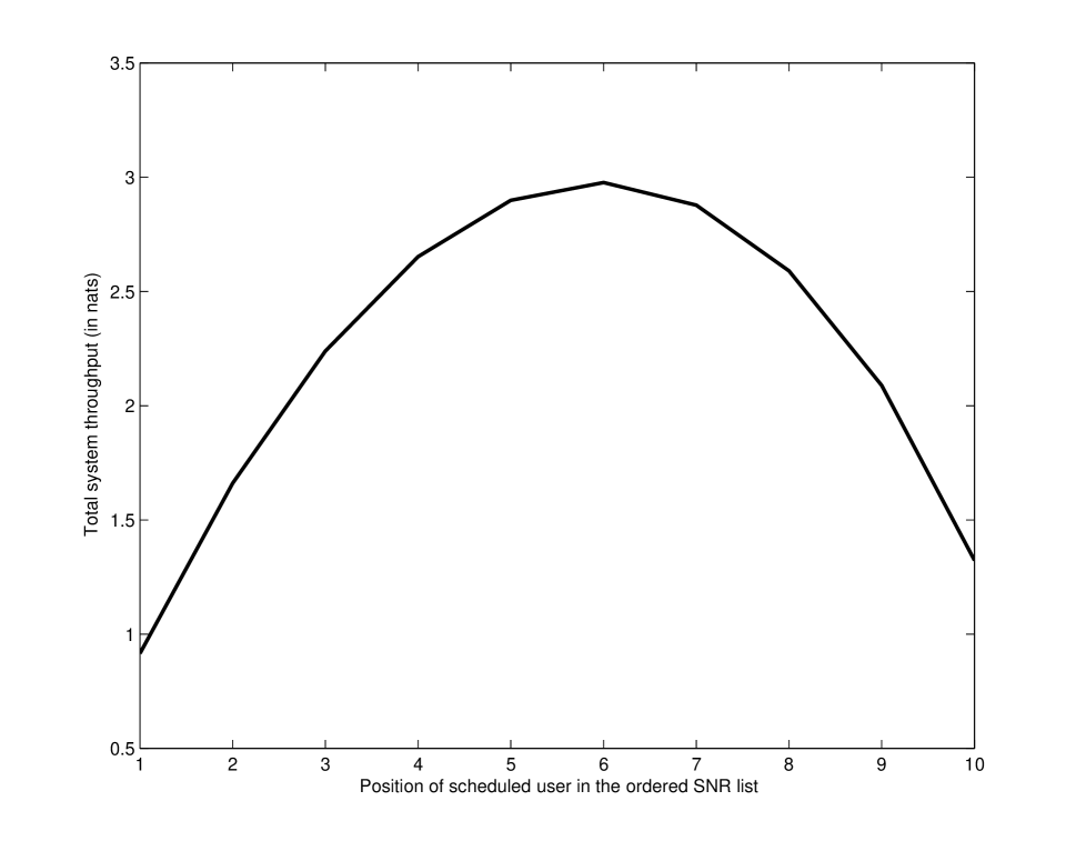
Figure 2: Throughput of the general static scheduling scheme for different positions of the intended user in the ordered list of SNRs of all users (N=10)

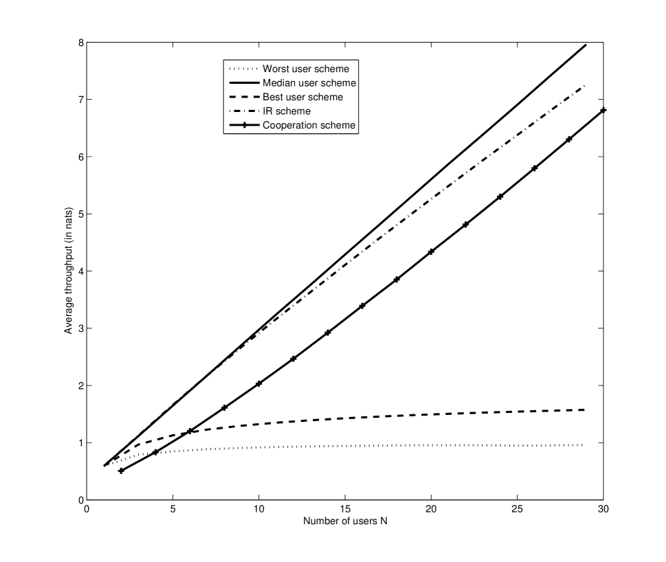
Figure 3: Comparison of the throughput of the proposed schemes

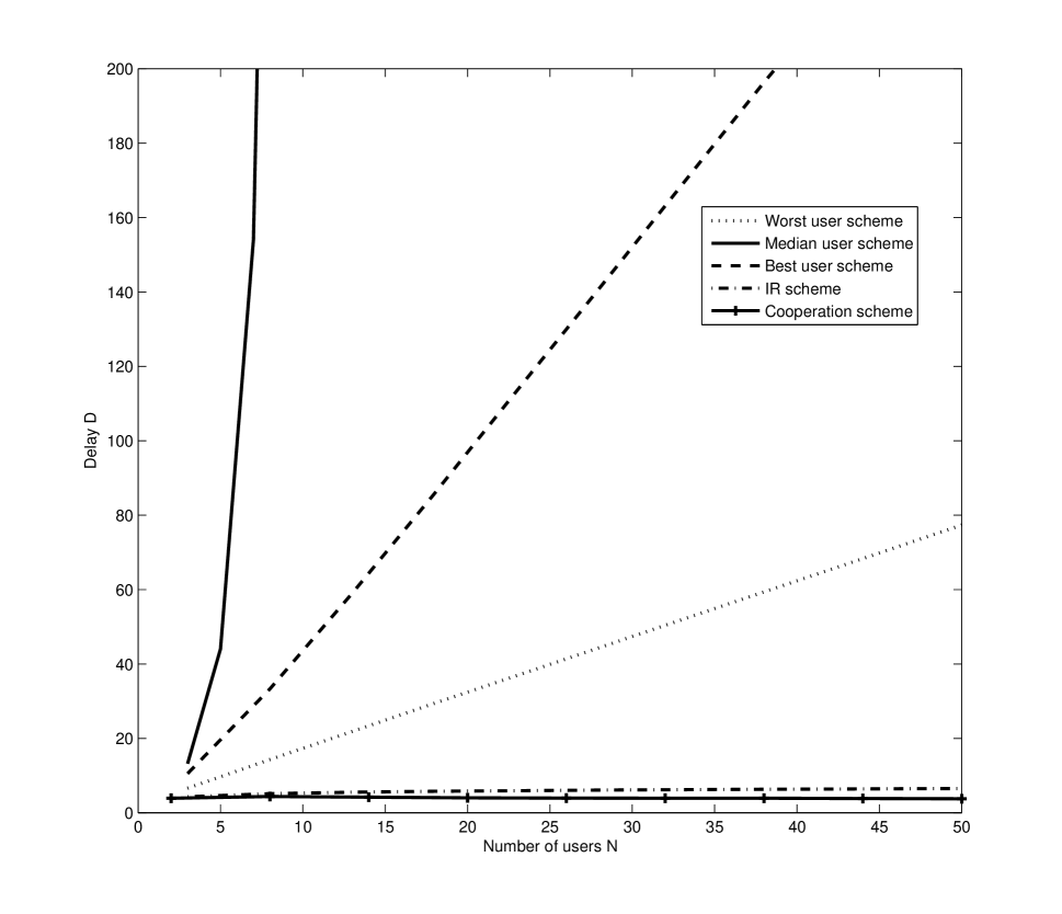
Figure 4: Comparison of the delay of the proposed schemes

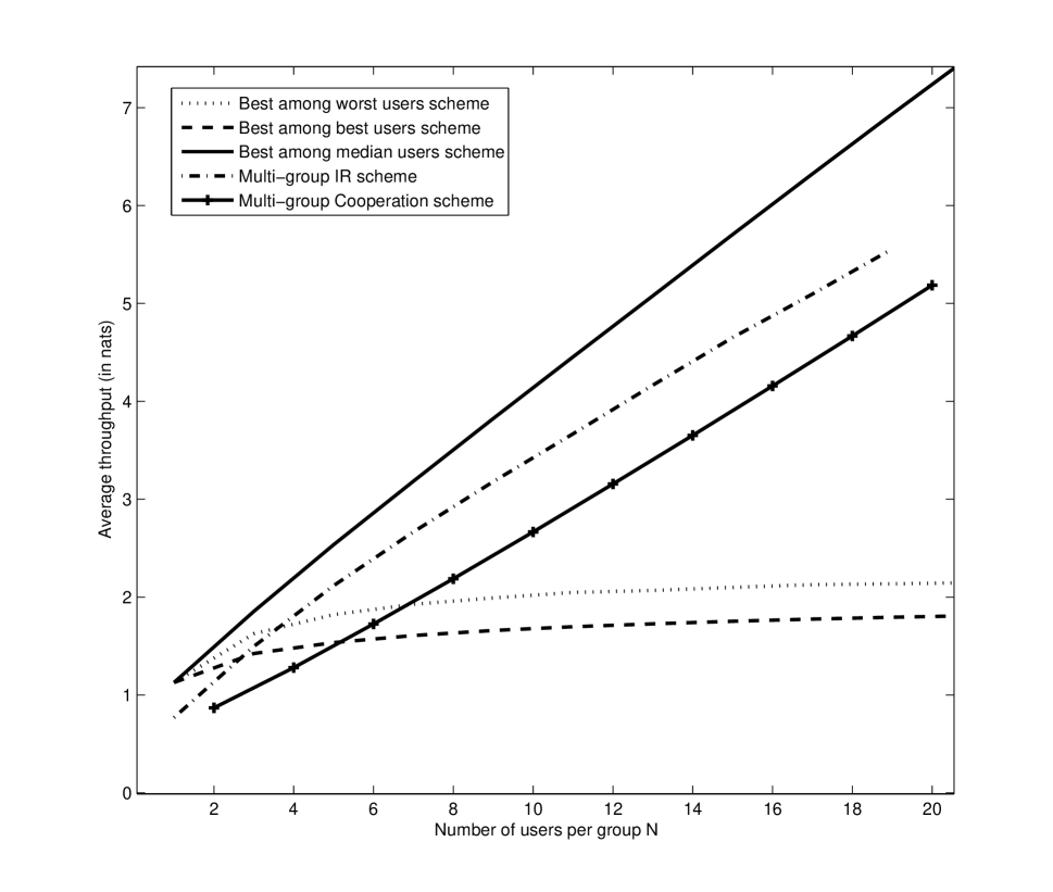
Figure 5: Comparison of the throughput of the proposed schemes for $G=5$ groups

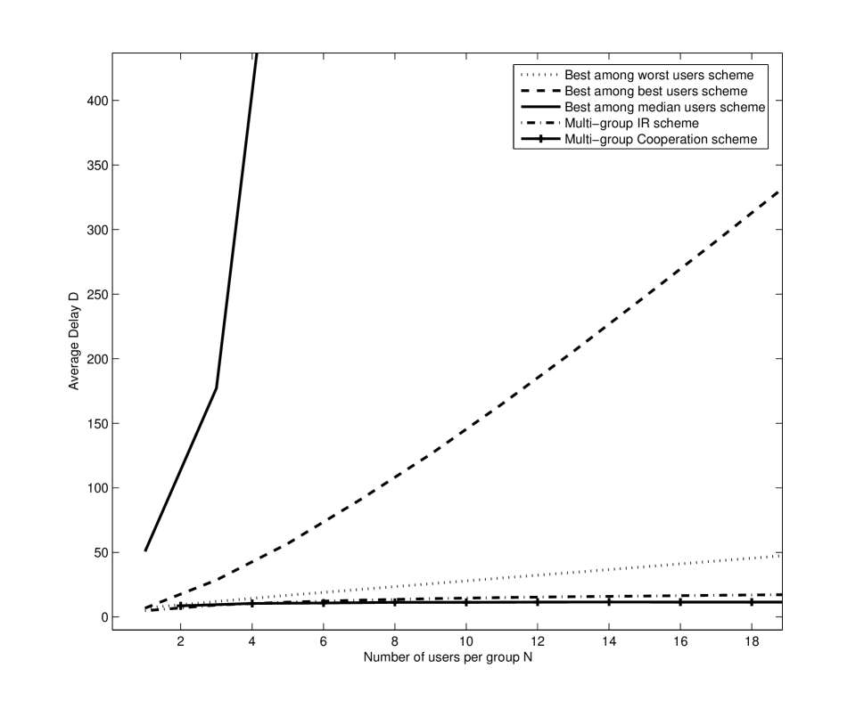
Figure 6: Comparison of the delay of the proposed schemes for $G=5$ groups

Here we present simulation results that validate our theoretical claims. These results were obtained through Monte-Carlo simulations and were averaged over at least 5000 iterations. The power constraint $P$ is taken to be unity. The throughput of the static schedulers, proposed in Section 3.1, is shown in Fig. 2 for different positions of the intended user in the ordered list of SNRs of all users. It is evident from the figure that, as predicted by the analysis, the throughput of the median user scheme is better than that of the best user scheme, which in turn outperforms the worst user scheme. In Fig. 3, we present a throughput-comparison for all the schemes proposed in Section 3 for increasing values of $N$. The corresponding delay-comparison is presented in Fig. 4. The throughput-comparison for the different scheduling schemes in the multi-group scenario is presented in Fig. 5 with $G=5$ groups (the corresponding delay-comparison is presented in Fig. 6). Although the best among worst users scheduler performs better than the best among best users scheme, in terms of throughput, for the range of $N$ values shown in the plot, it should be noted that the latter eventually outperforms the former for large values of $N$ ($N>600$). Except for this case, in all other considered scenarios, we can see that the simulation results follow the same trends predicted by our asymptotic analysis. Finally, we observe that the utility of our asymptotic analysis is manifested in its accurate predictions even with the relatively small number of users used in our simulations (i.e., in the order of $N=10$).

7 Conclusions

In this paper, we have used a cross layer design approach to shed more light on the throughput-delay tradeoff in the cellular multicast channel. Towards this end, we proposed three classes of scheduling algorithms with progressively increasing complexity, and analyzed the throughput-delay tradeoff achieved by each class. We first considered the class of low-complexity static scheduling schemes with memoryless decoding. We showed that a special case of this scheduling strategy, i.e., the median user scheduler, achieves the optimal scaling law of the throughput at the expense of an exponentially increasing delay with the number of users. We then proposed an incremental redundancy multicast scheme that achieves a superior throughput-delay tradeoff, at the expense of increased encoding/decoding complexity. We further proposed a cooperation scheme that achieves the optimal scaling laws of both throughput and delay at the expense of a high RF and computational complexity. We then generalized our schemes to the multi-group scenario and characterized their ability to exploit the multi-group diversity offered by the wireless channel. Finally, we presented simulation results that establish the accuracy of the predictions of our asymptotic analysis in systems with low to moderate number of users.

Appendix A Proof of Theorem 3

The channel gain $|h_{\pi(N-\frac{N}{\alpha}+1)}|^{2}$ has the distribution function $F(x)$ given by

$$F(x)=\sum_{k=(N-\frac{N}{\alpha}+1)}^{N}{N\choose k}(1-e^{-x})^{k}e^{-(N-k)x},\quad x\geq 0.$$

Hence the average throughput of the proposed scheme is given by

$$R_{tot}=\frac{N}{\alpha}\int_{0}^{\infty}\log(1+xP){\mathrm{d}}F(x).$$

Integrating by parts and simplifying, we obtain the average throughput as stated in equation (4) of the theorem.

We now calculate the average delay of the proposed scheme. We consider each coherence interval of length $T_{c}$ as a time slot. We first calculate the probability distribution of the service time $X$ required for transmitting a packet (of size $S$) when the base station always services the same queue. The service time $X$ is defined as

$$X=kT_{c},\qquad k\in\{1,2,\ldots\},$$ (28)

where $k$ is such that

$$T_{c}\left(\sum_{i=1}^{k-1}R_{\alpha}^{i}\right)<S\leq T_{c}\left(\sum_{i=1}^{k}R_{\alpha}^{i}\right).$$ (29)

Here $R_{\alpha}^{i}$ represents the service rate in the $i^{th}$ time slot as given in (3). The probability distribution of $X$ is given by

$$\textrm{Pr}(X=kT_{c})=\textrm{Pr}\left(\sum_{i=1}^{k-1}R_{\alpha}^{i}<\frac{S}{T_{c}}\leq\sum_{i=1}^{k}R_{\alpha}^{i}\right).$$

We let $C=(S/T_{c})$ in the sequel. Using the exponential server assumption in (2) for the service rates $\{R_{\alpha}^{i}\}$, we have (for $k\geq 1$)

$$\textrm{Pr}(X=kT_{c})=\int_{0}^{C}\left(f_{\left(R_{\alpha}^{1}+R_{\alpha}^{2}+\ldots+R_{\alpha}^{(k-1)}\right)}(y)dy\right)\textrm{Pr}(R_{\alpha}^{k}>C-y)$$

$$=\int_{0}^{C}\frac{e^{-\mu y}\mu^{k-1}y^{k-2}}{(k-2)!}e^{-\mu(C-y)}dy.$$

$$\Rightarrow\textrm{Pr}(X=kT_{c})=\frac{e^{-\mu C}(\mu C)^{k-1}}{(k-1)!},\qquad k\in\{1,2,\ldots\}.$$ (30)

Now the average service time $\bar{X}$ is given by

$$\bar{X}=\sum_{k=1}^{\infty}kT_{c}\textrm{Pr}(X=kT_{c})=\sum_{k=1}^{\infty}kT_{c}\left(\frac{e^{-\mu C}(\mu C)^{k-1}}{(k-1)!}\right).$$

$$\Rightarrow\bar{X}=(1+\mu C)T_{c}=T_{c}+\mu S.$$

Since $G=1$ for the single group scenario, the assumption in (1) reduces to

$$T_{c}=\Theta\left(\frac{1}{\log\log N}\right).$$

From the results in [19], we know that

$$E[R_{\alpha}]\leq E[R_{N}]=\Theta(\log\log N).$$

Hence

$$\mu=\frac{1}{E[R_{\alpha}]}=\Omega\left(\frac{1}{\log\log N}\right),\quad\forall 1\leq\alpha\leq N.$$

Thus for all possible values of the parameter $\alpha$, we have

$$\bar{X}=T_{c}+\mu S=\Theta(\mu S)=\Theta\left(\frac{1}{E[R_{\alpha}]}\right).$$

Hence it is clear that the assumption on $T_{c}$ in (1) ensures that the average service time $\bar{X}$ is not dominated by the scaling behaviour of $T_{c}$.

We now focus on one set of $\alpha$ coupled queues. Any packet that arrives into this set enters all the $\alpha$ queues within the set and moreover, the base station services only one of the ${N\choose N/\alpha}$ available queues in any time slot. Note that $\bar{X}$ was calculated assuming that the base station always services the same queue. We are interested in determining the delay involved in successfully transmitting a particular packet from all the $\alpha$ coupled queues in the set. The actual delay, as defined in Section 2, is the time between the start of transmission of a packet and the instant when the packet reaches all the $N$ users in the system. In our analysis, we assume that the packet of interest is at the head of all the $\alpha$ queues in the set during the start of transmission. This assumption thus yields a lower bound on the actual delay.

We characterize the delay based on the observation that our queuing problem is equivalent to the well-known “coupon collector” problem. This observation was made earlier in [14] where the authors characterized the delay of the throughput-optimal broadcast scheme. They assumed that the server (base station) offers a constant service rate which is independent of the instantaneous channel gains. In our analysis, however, we have incorporated the effects of rate adaptation. Let $X_{1},X_{2},\cdots,X_{\alpha}$ denote the service times (assuming continuous service), with distribution as given in (30), required for transmitting a packet from each of the $\alpha$ queues in the set. Then the delay of the proposed scheduling scheme is directly proportional to the minimum number of trials required to ensure that the first queue is served at least $(X_{1}/T_{c})$ times by the base station, the second queue is served at least $(X_{2}/T_{c})$ times and so on …

We lower bound the average delay by calculating the minimum number of trials $N_{t}$ required to ensure that all the $\alpha$ queues are served at least $(X_{min}/T_{c})$ times by the base station, where $X_{min}=\min\{X_{1},X_{2},\cdots,X_{\alpha}\}$. We determine the average number of such required trials $E[N_{t}|X_{min}]$ using the results derived in [14]. Since the base station services only one of the ${N\choose N/\alpha}$ queues in any time slot and the users are symmetric, there is an equal probability that the base station services any one of the queues. Since we need to consider only one set of $\alpha$ coupled queues for determining the delay, we consider all the other queues in the system jointly as one “dummy” queue called the $(\alpha+1)^{th}$ queue. Now the probabilities $\{p_{j}\}$ of the server choosing the $j^{th}$ queue is given by

$$p_{1}=\cdots=p_{\alpha}=\frac{1}{{N\choose N/\alpha}}\quad\textrm{and}\quad p_{\alpha+1}=P_{e}=1-\frac{\alpha}{{N\choose N/\alpha}}.$$

These probabilities $\{p_{j}\}$ remain constant through all time slots and are not functions of the instantaneous service rates $\{R_{\alpha}^{i}\}$ provided by the base station. The Moment Generating Function (MGF) of the number of trials required is given by [14]

$$F_{N_{t}|X_{min}}(z)=\sum_{i=0}^{\infty}z^{i}\textrm{Pr}(N_{t}>i)=\sum_{i=0}^{\infty}z^{i}b_{i},$$

where $b_{i}$ is the probability of failure of sending a packet to all the users in $i$ channel uses. The value of $b_{i}$ is equal to the polynomial

$$\left(\frac{x_{1}}{{N\choose N/\alpha}}+\cdots+\frac{x_{\alpha}}{{N\choose N/\alpha}}+P_{e}x_{\alpha+1}\right)^{i}$$

evaluated at $x_{1}=\cdots=x_{\alpha+1}=1$ after removing the terms that have all exponents of $x_{1},\cdots,x_{\alpha}$ greater than or equal to $(X_{min}/T_{c})$ (denoted by the operator $\{.\}$). Thus the MGF of the number of trials required is given by

$$F_{N_{t}|X_{min}}(z)=\sum_{i=0}^{\infty}\frac{z^{i}}{\left[{N\choose N/\alpha}\right]^{i}}\left\{\left(x_{1}+\cdots+x_{\alpha}+P_{e}{N\choose N/\alpha}x_{\alpha+1}\right)^{i}\right\}$$

evaluated at $x_{1}=\cdots=x_{\alpha+1}=1$. But we know that

$$\frac{i!z^{i}}{\left[{N\choose N/\alpha}\right]^{i}}=\frac{{N\choose N/\alpha}}{z}\int_{0}^{\infty}e^{-\frac{{N\choose N/\alpha}t}{z}}t^{i}dt.$$

Using this identity and simplifying, we get

$$F_{N_{t}|X_{min}}(z)=\frac{{N\choose N/\alpha}}{z}\int_{0}^{\infty}e^{-\frac{{N\choose N/\alpha}t}{z}}\left(e^{{N\choose N/\alpha}t}\left[1-\left(1-S_{\left(\frac{X_{min}}{T_{c}}\right)}(t)e^{-t}\right)^{\alpha}\right]\right)dt,$$

where

$$S_{m}(t)=\sum_{i=0}^{m-1}\frac{t^{i}}{i!}.$$

Hence the average number of trials required $E[N_{t}|X_{min}]$ is given by [14]

$$E[N_{t}|X_{min}]=F_{N_{t}|X_{min}}(1)={N\choose N/\alpha}\int_{0}^{\infty}\left[1-\left(1-S_{\left(\frac{X_{min}}{T_{c}}\right)}(t)e^{-t}\right)^{\alpha}\right]dt={N\choose N/\alpha}E\left[\max_{1\leq i\leq\alpha}Y_{i}\right],$$

where the $Y_{i}$’s are i.i.d random variables that follow a Chi-square distribution with $(2X_{min}/T_{c})$ degrees of freedom. From the results in [14], it can be seen that for such a sequence of random variables $\{Y_{i}\}$,

$$E\left[\max_{1\leq i\leq\alpha}Y_{i}\right]=\max\left\{\Theta(\log\alpha),\Theta\left(\frac{X_{min}}{T_{c}}\right)\right\}.$$ (31)

Using this result, the average number of trials required is given by

$$E[N_{t}|X_{min}]=\max\left\{\Theta\left({N\choose N/\alpha}\log\alpha\right),\Theta\left({N\choose N/\alpha}\frac{X_{min}}{T_{c}}\right)\right\}.$$

Thus the average delay of the general static scheduling scheme can be lower bounded by

$$D\geq E_{X_{min}}\left[E[N_{t}|X_{min}]T_{c}\right]\quad=E_{X_{min}}\left[\max\left\{\Theta\left({N\choose N/\alpha}T_{c}\log\alpha\right),\Theta\left({N\choose N/\alpha}X_{min}\right)\right\}\right].$$

Since $E\left[\max\{Z_{1},Z_{2}\}\right]\geq\max\left\{E[Z_{1}],E[Z_{2}]\right\}$, we have

$$D=\max\left\{\Omega\left({N\choose N/\alpha}T_{c}\log\alpha\right),\Omega\left({N\choose N/\alpha}E[X_{min}]\right)\right\}.$$

$$\Rightarrow D=\max\left\{\Omega\left({N\choose N/\alpha}\frac{\log\alpha}{\log\log N}\right),\Omega\left({N\choose N/\alpha}E[X_{min}]\right)\right\}.$$ (32)

Moreover, when $E[X_{min}]=\Theta\left(\bar{X}\right)$, it can be easily seen that the expression on the right in (32) gives the exact scaling of the average delay $D$, instead of just being a lower bound for it.

Appendix B Proof of Lemma 4

The average throughput of the worst user scheme is given by

$$R_{tot}=N\int_{0}^{\infty}\log(1+xP)Ne^{-Nx}{\mathrm{d}}x=-Ne^{\left(\frac{N}{P}\right)}Ei\left(-\frac{N}{P}\right).$$ (33)

For large values of $x$, we have

$$Ei(-x)=\int_{-\infty}^{-x}\frac{e^{t}}{t}{\mathrm{d}}t=-\frac{e^{-x}}{x}\left(1+\epsilon\right),$$

where $\epsilon\to 0$ as $x\to\infty$. Using this in (33), we get

$$R_{tot}=P(1+\epsilon)=\Theta(1).$$

Letting $\alpha=1$ in (5) of Theorem 3, we get the average delay as

$$D=\max\left\{\Omega\left(\frac{1}{\log\log N}\right),\Omega\left(E[X_{min}]\right)\right\}.$$ (34)

Since the base station maintains only a single queue for the worst user scheme, we have

$$E[X_{min}]=\bar{X}=\Theta\left(\frac{1}{E[R_{1}]}\right).$$

The average service rate $E[R_{1}]$ is given by

$$E[R_{1}]=\int_{0}^{\infty}\log(1+xP)Ne^{-Nx}{\mathrm{d}}x=-e^{\left(\frac{N}{P}\right)}Ei\left(-\frac{N}{P}\right)=\Theta\left(\frac{1}{N}\right).$$

Since $E[X_{min}]=\bar{X}$, the expression on the right in (34) gives the exact scaling of $D$. Thus the average delay of the worst user scheme scales as $D=\Theta(N)$.

Appendix C Proof of Lemma 5

By letting $\alpha=N$ in (4) of Theorem 3, the average throughput of the best user scheme is found to be

$$R_{tot}=\sum_{i=1}^{N}{N\choose i}(-1)^{i}e^{\left(\frac{i}{P}\right)}Ei\left(\frac{-i}{P}\right).$$ (35)

It has been shown in [19] that the throughput in (35) scales as

$$R_{tot}=\Theta(\log\log N)$$ (36)

with the number of users $N$. Hence the average service rate is given by

$$E[R_{N}]=R_{tot}=\Theta\left(\log\log N\right).$$

Letting $\alpha=N$ in (5) of Theorem 3, we get the average delay as

$$D=\max\left\{\Omega\left(\frac{N\log N}{\log\log N}\right),\Omega\left(NE[X_{min}]\right)\right\}.$$ (37)

Now

$$E[X_{min}]=E\left[\min_{i=1}^{N}X_{i}\right]\leq\bar{X}=\Theta\left(\frac{1}{E[R_{N}]}\right).$$

Hence

$$E[X_{min}]=O\left(\frac{1}{\log\log N}\right).$$

Thus, from (37), the average delay of the best user scheme scales as

$$D=\Omega\left(\frac{N\log N}{\log\log N}\right).$$

Appendix D Proof of Lemma 6

The average throughput of the median user scheme can be derived by letting $\alpha=2$ in (4) of Theorem 3. From the results on central order statistics in [20] (Theorem 8.5.1), we know that the sample median of $N$ i.i.d. exponential random variables converges in distribution to a normal random variable with mean $\theta$ and variance $(1/N)$, where $\theta=\log 2$ is the median of the underlying exponential distribution. Hence

$$\left(|h_{\pi(\frac{N}{2}+1)}|^{2}-\theta\right)\sqrt{N}\to W\quad\textrm{in distribution},$$

where $W$ is a standard normal random variable. Using Chebyshev’s inequality, we get $\forall\epsilon>0$

$$\textrm{Pr}\left(\left||h_{\pi(\frac{N}{2}+1)}|^{2}-\theta\right|>\epsilon\right)=\textrm{Pr}\left(\sqrt{N}\left||h_{\pi(\frac{N}{2}+1)}|^{2}-\theta\right|>\epsilon\sqrt{N}\right)<\frac{E[W^{2}]+\delta}{N\epsilon^{2}}\to 0\quad\textrm{as $N\to\infty$}.$$

$$\Rightarrow|h_{\pi(\frac{N}{2}+1)}|^{2}\to\theta\quad\textrm{in probability}.$$

Since the $\log(.)$ function is continuous, we have

$$\log\left(1+|h_{\pi(\frac{N}{2}+1)}|^{2}P\right)\to\log(1+\theta P)\quad\textrm{in probability}.$$ (38)

We now derive a lower bound on the average throughput. We recall the following property of positive random variables. Let $(X_{n})$ be a set of positive random variables converging to a constant $A$ in probability. Hence $\forall\epsilon>0$,

$$\textrm{Pr}\left(|X_{n}-A|\geq\epsilon\right)<\delta,$$

for some small $\delta>0$. Now

$$E[X_{n}]=\int_{0}^{\infty}tf_{X_{n}}(t){\mathrm{d}}t\quad\geq\int_{A-\epsilon}^{A+\epsilon}tf_{X_{n}}(t){\mathrm{d}}t\quad\geq(A-\epsilon)(1-\delta).$$

Taking the limit as $n\to\infty$, we get

$$\lim_{n\to\infty}E[X_{n}]\geq A.$$ (39)

Using this property in (38), we get

$$\lim_{N\to\infty}E\left[\log\left(1+|h_{\pi(\frac{N}{2}+1)}|^{2}P\right)\right]\geq\log(1+\theta P)=\Theta(1).$$

$$\Rightarrow R_{tot}=\left(\frac{N}{2}\right)E\left[\log\left(1+|h_{\pi(\frac{N}{2}+1)}|^{2}P\right)\right]=\Omega(N).$$ (40)

An upper bound on the average throughput of any scheduling scheme is given by

$$R_{tot}\leq E\left[\sum_{i=1}^{N}\log\left(1+|h_{i}|^{2}P\right)\right]=NE\left[\log\left(1+|h_{1}|^{2}P\right)\right].$$

Hence

$$R_{tot}=O(N).$$ (41)

Combining this with the lower bound in (40), we get

$$R_{tot}=\Theta(N).$$

Thus it is clear that the throughput of the proposed median user scheme is scaling law optimal. Letting $\alpha=2$ in (5) of Theorem 3, we get the average delay as

$$D=\max\left\{\Omega\left({N\choose N/2}\frac{1}{\log\log N}\right),\Omega\left({N\choose N/2}E[X_{min}]\right)\right\}.$$ (42)

Now, since $X_{min}=\min\{X_{1},X_{2}\}$, we have

$$E[X_{min}]=\Theta\left(\bar{X}\right)=\Theta\left(\frac{1}{E[R_{2}]}\right).$$

The average service rate $E[R_{2}]$ is given by

$$E[R_{2}]=E\left[\log\left(1+|h_{\pi(\frac{N}{2}+1)}|^{2}P\right)\right]=\Theta(1).$$ (43)

Since $E[X_{min}]=\Theta\left(\bar{X}\right)$, the expression on the right in (42) gives the exact scaling of $D$. Thus the average delay of the median user scheme scales as

$$D=\Theta\left({N\choose N/2}\right).$$

Using Stirling’s formula, we obtain the scaling of the average delay as given in (11).

Appendix E Proof of Theorem 7

Let $A_{i}$ denote the event that a packet is successfully decoded by all the $N$ users in the system in $i$ transmission attempts. Following the notation in [18], we define

$$q(m)=\textrm{Pr}(\overline{A_{1}},\ldots,\overline{A_{m-1}},A_{m})=p(m-1)-p(m),$$

where

$$p(m)=\textrm{Pr}(\overline{A_{1}},\ldots,\overline{A_{m-1}},\overline{A_{m}})=1-\sum_{l=1}^{m}q(l),$$

with $p(0)=1$. The rate $\bar{R}$ is defined as $\bar{R}=(b/L)$. We define the random variable $\tau$ to be the number of transmission attempts made between the instant when the codeword is generated and the instant when its transmission is stopped (Transmission is stopped either when the packet is successfully decoded by all the $N$ users or the number of transmission attempts exceeds the rate constraint $M$). The probability distribution of $\tau$ is given by

$$f_{\tau}(m)=\left\{\begin{array}[]{l}0,\quad m=0\\ q(m),\quad 1\leq m\leq M-1\\ q(M)+p(M),\quad m=M\end{array}\right.$$

We define the random reward ${\mathcal{R}}$ as follows: ${\mathcal{R}}=N\bar{R}$ if transmission stops because of successful decoding and ${\mathcal{R}}=0$ if transmission stops because of the rate constraint violation. Hence

$$E[{\mathcal{R}}]=N\bar{R}\sum_{m=1}^{M}q(m)=N\bar{R}[1-p(M)].$$

The mean inter-renewal time is given by

$$E[\tau]=\sum_{m=1}^{M}mf_{\tau}(m)=\sum_{m=1}^{M}mq(m)+Mp(M)=\sum_{m=1}^{M}m[p(m-1)-p(m)]+Mp(M)=\sum_{m=0}^{M-1}p(m).$$

Applying the renewal-reward theorem, we obtain the average throughput of the proposed scheme as

$$R_{tot}=\frac{E[{\mathcal{R}}]}{E[\tau]},\quad\textrm{with probability $1$}.$$

Hence

$$R_{tot}=\frac{N\bar{R}\left[1-p(M)\right]}{1+\sum_{m=1}^{M-1}p(m)}.$$

The average delay $D$ of the scheme is given by the mean inter-renewal time. Hence

$$D=E[\tau]=1+\sum_{m=1}^{M-1}p(m).$$

The unconstrained throughput and delay of this scheme are obtained by letting $M\to\infty$ and are given by

$$R_{tot}=\frac{N\bar{R}}{\sum_{m=0}^{\infty}p(m)},$$ (44)

and

$$D=\sum_{m=0}^{\infty}p(m).$$ (45)

From the earlier definitions, we have

$$p(m)=\textrm{Pr}(\overline{A_{1}},\ldots,\overline{A_{m-1}},\overline{A_{m}})=\textrm{Pr}(\overline{A_{m}})=\textrm{Pr}\left(\min_{i=1}^{N}\sum_{k=1}^{m}I(X;Y_{ik})\leq\bar{R}\right).$$

$$\Rightarrow p(m)=1-\textrm{Pr}\left(\min_{i=1}^{N}\sum_{k=1}^{m}I(X;Y_{ik})>\bar{R}\right)=1-\left[1-\textrm{Pr}\left(\sum_{k=1}^{m}I(X;Y_{1k})\leq\bar{R}\right)\right]^{N}.$$ (46)

Now for a Gaussian input distribution, we have

$$\sum_{k=1}^{m}I(X;Y_{1k})=\sum_{k=1}^{m}\log(1+|h_{k}|^{2}).$$

We know that

$$\log\left(1+\sum_{k=1}^{m}|h_{k}|^{2}\right)\leq\sum_{k=1}^{m}\log(1+|h_{k}|^{2})\leq\sum_{k=1}^{m}|h_{k}|^{2}.$$

Hence

$$\textrm{Pr}\left(\sum_{k=1}^{m}|h_{k}|^{2}\leq(e^{\bar{R}}-1)\right)\geq\textrm{Pr}\left(\sum_{k=1}^{m}\log(1+|h_{k}|^{2})\leq\bar{R}\right)\geq\textrm{Pr}\left(\sum_{k=1}^{m}|h_{k}|^{2}\leq\bar{R}\right).$$

Since both $\bar{R}$ and $(e^{\bar{R}}-1)$ are constants, substituting both the lower and upper bounds in (46) will yield the same scaling with $N$. So we consider only the lower bound on $p(m)$. Let

$$s(m)=1-\left[1-\textrm{Pr}\left(\sum_{k=1}^{m}|h_{k}|^{2}\leq\bar{R}\right)\right]^{N}.$$

Hence

$$\sum_{m=0}^{\infty}p(m)=\Theta\left(\sum_{m=0}^{\infty}s(m)\right)\quad\textrm{w.r.t $N$}.$$

The random variable $\sum_{k=1}^{m}|h_{k}|^{2}$ has a $2m$-dimensional Chi-square distribution with the density and distribution functions given by

$$f(x)=\frac{e^{-x}x^{m-1}}{(m-1)!},\quad x\geq 0$$

and

$$F(x)=1-e^{-x}\left(\sum_{l=0}^{m-1}\frac{x^{l}}{l!}\right),\quad x\geq 0.$$

Hence

$$s(m)=1-\left[e^{-\bar{R}}\left(\sum_{l=0}^{m-1}\frac{\bar{R}^{l}}{l!}\right)\right]^{N}.$$

From Taylor’s theorem, we know that (for some $0<\theta<1$)

$$e^{\bar{R}}=\sum_{l=0}^{m-1}\frac{\bar{R}^{l}}{l!}+\frac{e^{\theta\bar{R}}{\bar{R}}^{m}}{m!}\quad\Rightarrow\sum_{l=0}^{m-1}\frac{\bar{R}^{l}}{l!}=e^{\bar{R}}-\frac{e^{\theta\bar{R}}{\bar{R}}^{m}}{m!}.$$

$$\Rightarrow s(m)=1-\left(1-\frac{e^{-(1-\theta)\bar{R}}\bar{R}^{m}}{m!}\right)^{N}.$$

To find the scaling of $\sum_{m=0}^{\infty}s(m)$ w.r.t $N$, we first derive a lower bound by finding the value of $m$ until which $s(m)\to 1$ as $N\to\infty$. Now

$$s(m)\to 1\quad\Rightarrow\left(1-\frac{e^{-(1-\theta)\bar{R}}\bar{R}^{m}}{m!}\right)^{N}\to 0.$$

$$\Rightarrow\frac{e^{-(1-\theta)\bar{R}}\bar{R}^{m}}{m!}>\Theta\left(\frac{1}{N}\right).$$

Using Stirling’s approximation, we have

$$\frac{e^{-(1-\theta)\bar{R}}\bar{R}^{m}}{\sqrt{2\pi m}e^{-m}m^{m}}>\frac{k}{N},\quad\forall\quad\textrm{constant $k$}.$$

Taking log on both sides, we get

$$(1-\theta)\bar{R}-m+m\log\left(\frac{m}{\bar{R}}\right)+\frac{1}{2}\log(2\pi m)<\log N-\log k,\quad\forall k.$$

For large $N$, this equation can be reduced to

$$m\log m<\log N.$$ (47)

This equation is satisfied by all values of $m$ such that

$$m<\Theta\left(\frac{\log N}{\log\log N}\right).$$

Since $s(m)\to 1$ as $N\to\infty$ for all values of $m$ that satisfy the above equation, the sum of $s(m)$’s can be lower bounded as

$$\sum_{m=0}^{\infty}s(m)\geq\Theta\left(\frac{\log N}{\log\log N}\right).$$ (48)

Similarly an upper bound on $\sum_{m=0}^{\infty}s(m)$ can be derived by finding the value of $m$ from which $s(m)\to 0$ as $N\to\infty$. Following the same procedure as before, we find that $s(m)\to 0$ when

$$m>\Theta\left(\frac{\log N}{\log\log N}\right).$$

This yields the following upper bound

$$\sum_{m=0}^{\infty}s(m)\leq\Theta\left(\frac{\log N}{\log\log N}\right).$$

Combining this with the lower bound in (48), we get

$$\sum_{m=0}^{\infty}s(m)=\Theta\left(\frac{\log N}{\log\log N}\right).$$

Thus the average delay is given by

$$D=\sum_{m=0}^{\infty}p(m)=\Theta\left(\sum_{m=0}^{\infty}s(m)\right)=\Theta\left(\frac{\log N}{\log\log N}\right).$$

The average throughput of the incremental redundancy scheme is then given by

$$R_{tot}=\frac{N\bar{R}}{\sum_{m=0}^{\infty}p(m)}=\frac{N\bar{R}}{D}=\Theta\left(\frac{N\log\log N}{\log N}\right).$$

Appendix F Proof of Theorem 8

The first stage of the cooperation scheme is the median user scheme. Hence it is clear from (10) that

$$E[R_{s1}]=E\left[\log\left(1+|h_{\pi(\frac{N}{2}+1)}|^{2}P\right)\right]=\Theta(1).$$

As noted earlier, the cooperative transmission by the users in the second stage is equivalent to the transmission of packets from a transmitter equipped with $(N/2)$ transmit antennas to the worst user in a group of $(N/2)$ users. Hence the average transmission rate during the cooperative stage is given by

$$E[R_{s2}]=E\left[\min_{i=1,...,(N/2)}\log\left(1+\frac{|h_{1i}|^{2}+\cdots+|h_{(N/2)i}|^{2}}{(N/2)}P\right)\right],$$

where the $|h_{ki}|^{2}$’s are i.i.d and exponentially distributed and represent the inter-user fading coefficients.

$$\Rightarrow E[R_{s2}]=E\left[\log\left(1+\min_{i=1,...,M}\frac{|\chi^{i}_{2M}|^{2}}{M}P\right)\right],$$ (49)

where $M=(N/2)$ and $|\chi^{i}_{2M}|^{2}$’s are Chi-square random variables with $2M$ degrees of freedom whose distribution function is given by

$$F(x)=1-e^{-x}\left(\sum_{j=0}^{M-1}\frac{x^{j}}{j!}\right),\quad x\geq 0.$$

Using the results on extreme order statistics in [20] (Theorems 8.3.2-8.3.6), it can be shown that the random variable

$$\frac{\min_{i=1}^{M}|\chi^{i}_{2M}|^{2}}{b_{M}}\quad\to\quad W\quad\textrm{in distribution as $M\to\infty$},$$

where $W$ is a Weibull type random variable and $b_{M}$ satisfies $F(b_{M})=\frac{1}{M}$. Now

$$F(b_{M})=\frac{1}{M}\quad\Rightarrow 1-e^{-b_{M}}\left(\sum_{j=0}^{M-1}\frac{b_{M}^{j}}{j!}\right)=\frac{1}{M}.$$

Using Taylor’s theorem, we get for some $0<\beta_{M}<1$

$$1-e^{-b_{M}}\left(e^{b_{M}}-\frac{e^{\beta_{M}b_{M}}b_{M}^{M}}{M!}\right)=\frac{1}{M}\quad\Rightarrow\frac{e^{-(1-\beta_{M})b_{M}}b_{M}^{M}}{M!}=\frac{1}{M}.$$

Using Stirling’s approximation, we have

$$\frac{e^{-(1-\beta_{M})b_{M}}b_{M}^{M}}{\sqrt{2\pi M}M^{M}e^{-M}}=\frac{1}{M}.$$

Taking $\log(.)$ on both sides, we get

$$(1-\beta_{M})b_{M}-M\log b_{M}=M-\left(M-\frac{1}{2}\right)\log M+C.$$

Since $\beta_{M}\to 0$ as $M\to\infty$, we get $b_{M}=\Theta(M)$. Thus

$$\frac{\min_{i=1}^{M}|\chi^{i}_{2M}|^{2}}{M}\to kW\quad\textrm{in distribution, for some constant $k>0$}.$$

Since the $\log(.)$ function is continuous, we have

$$\log\left(1+\frac{\min_{i=1}^{M}|\chi^{i}_{2M}|^{2}}{M}P\right)\to\log(1+kWP)\quad\textrm{in distribution, as $M\to\infty$}.$$

Now, we know

$$\log\left(1+\frac{\min_{i=1}^{M}|\chi^{i}_{2M}|^{2}}{M}P\right)\leq\frac{\left(\min_{i=1}^{M}|\chi^{i}_{2M}|^{2}\right)P}{M}\leq\frac{|\chi^{1}_{2M}|^{2}P}{M}.$$

Since

$$E\left[\left(\frac{|\chi^{1}_{2M}|^{2}P}{M}\right)^{2}\right]=\frac{E[(|\chi^{1}_{2M}|^{2})^{2}]P^{2}}{M^{2}}=\left(\frac{M^{2}+M}{M^{2}}\right)P^{2}=\left(1+\frac{1}{M}\right)P^{2}\leq 2P^{2}<\infty\quad\forall M,$$

$$\Rightarrow\left\{\frac{|\chi^{1}_{2M}|^{2}P}{M};M\geq 1\right\}\quad\textrm{is uniformly integrable.}$$

$$\Rightarrow\left\{\log\left(1+\frac{\min_{i=1}^{M}|\chi^{i}_{2M}|^{2}}{M}P\right);M\geq 1\right\}\quad\textrm{is uniformly integrable.}$$

It is shown in [21] that if a sequence of random variables $(X_{n})$ is uniformly integrable and $X_{n}\to X$ in distribution as $n\to\infty$, then $EX_{n}\to EX$ as $n\to\infty$. Thus

$$E\left[\log\left(1+\frac{\min_{i=1}^{M}|\chi^{i}_{2M}|^{2}}{M}P\right)\right]\to E[\log(1+kWP)]=\Theta(1).$$

Hence the average transmission rate of the second stage is given by $E[R_{s2}]=\Theta(1)$ w.r.t $N$. Since both $E[R_{s1}]$ and $E[R_{s2}]$ do not scale with $N$ and since the minimum is taken over only two positive quantities, we have

$$E\left[\min\{R_{s1},R_{s2}\}\right]=\Theta\left(E[R_{s1}]\right)=\Theta(1).$$

Thus the average throughput of the cooperation scheme is given by

$$R_{tot}=\left(\frac{N}{2}\right)E\left[\min\{R_{s1},R_{s2}\}\ \right]=\Theta(N).$$

We now determine the average delay of the cooperation scheme. We note that the base station needs to maintain only a single queue that caters to all the $N$ users in the system. The information transmitted by the base station in the first half of each time slot reaches all the $N$ users at the end of that time slot. Hence the average delay is equal to the average service time required for transmitting a packet of size $S$ from the queue. Following the steps in Appendix A, the average delay $D$ for transmitting a packet in the cooperation scheme is given by

$$D=T_{c}+\mu S=\Theta\left(\frac{S}{E[\min\{R_{s1},R_{s2}\}]}\right)=\Theta(1).$$

Appendix G Proof of Theorem 9

We first extend the proof of the general static scheduling scheme given in Appendix A to the multi-group scenario and then consider the three special cases. The average throughput $R_{tot}$ of the general multi-group scheduling scheme is given by

$$R_{tot}=\left(\frac{N}{\alpha}\right)E[R_{\alpha}],$$

where $R_{\alpha}$ represents the transmission rate to each of the intended $(N/\alpha)$ users and is given by

$$R_{\alpha}=\log\left(1+|h_{bg}|^{2}P\right),$$

where the distribution of $|h_{bg}|^{2}$ is given by

$$F_{bg}(x)=\left(\sum_{k=(N-\frac{N}{\alpha}+1)}^{N}{N\choose k}\left(1-e^{-x}\right)^{k}e^{-(N-k)x}\right)^{G},\forall x\geq 0.$$ (50)

Hence the average throughput is given by

$$R_{tot}=\frac{N}{\alpha}\int_{0}^{\infty}\log(1+xP){\mathrm{d}}F_{bg}(x).$$ (51)

Integrating by parts and simplifying, we obtain the average throughput of the proposed scheme.

For implementing the general multi-group static scheduling scheme, the base station needs to maintain $G{N\choose N/\alpha}$ queues, one for each combination of $(N/\alpha)$ users in each of the $G$ groups. These queues can be divided into $G$ sets, one for each of the groups. Within each set corresponding to a particular group, the queues can be further divided into subsets with $\alpha$ coupled queues in each subset such that the combinations of users served by the $\alpha$ queues within a subset are mutually exclusive and collectively exhaustive (i.e., every user in the particular group is served by exactly one of the $\alpha$ queues). We consider one such subset of $\alpha$ queues corresponding to any one of the $G$ groups. Any packet that arrives into the subset enters all the $\alpha$ queues since it needs to be transmitted to all the users within the group. At any instant of time, the base station services only one of the $G{N\choose N/\alpha}$ queues.

As before, we first calculate the average service time $\bar{X}$ required for transmitting a packet by assuming that the base station always services the same queue. Following the steps in Appendix A, the average service time $\bar{X}$ is given by

$$\bar{X}=T_{c}+\mu S=\Theta\left(\frac{S}{E[R_{\alpha}]}\right).$$

We again use the results in [14] to derive a lower bound on the actual delay by considering the minimum number of trials $N_{t}$ required to ensure that all the $\alpha$ queues are served at least $(X_{min}/T_{c})$ times by the base station. As before, we consider only $(\alpha+1)$ queues with the $(\alpha+1)^{th}$ queue being the “dummy” queue representing all the queues in all other subsets in the system. Now the probabilities $\{p_{i}\}$ of the server choosing the $i^{th}$ queue are given by

$$p_{1}=\cdots=p_{\alpha}=\frac{1}{G{N\choose N/\alpha}}\quad\textrm{and}\quad p_{\alpha+1}=1-\frac{\alpha}{G{N\choose N/\alpha}}.$$

Proceeding as in Appendix A, the MGF of the number of trials required is given by

$$F_{N_{t}|X_{min}}(z)=\frac{G{N\choose N/\alpha}}{z}\int_{0}^{\infty}e^{-\frac{G{N\choose N/\alpha}t}{z}}\left(e^{G{N\choose N/\alpha}t}\left[1-\left(1-S_{\left(\frac{X_{min}}{T_{c}}\right)}(t)e^{-t}\right)^{\alpha}\right]\right)dt.$$

The average number of trials required $E[N_{t}|X_{min}]$ is given by

$$E[N_{t}|X_{min}]=F_{N_{t}|X_{min}}(1)=G{N\choose N/\alpha}\int_{0}^{\infty}\left[1-\left(1-S_{\left(\frac{X_{min}}{T_{c}}\right)}(t)e^{-t}\right)^{\alpha}\right]dt=G{N\choose N/\alpha}E\left[\max_{1\leq i\leq\alpha}Y_{i}\right],$$

where the $Y_{i}$’s are i.i.d random variables that follow a Chi-square distribution with $(2X_{min}/T_{c})$ degrees of freedom. Using the result in (31), we get

$$E[N_{t}|X_{min}]=\max\left\{\Theta\left(G{N\choose N/\alpha}\log\alpha\right),\Theta\left(G{N\choose N/\alpha}\frac{X_{min}}{T_{c}}\right)\right\}.$$

Thus the average delay of the proposed scheme can be lower bounded as

$$D\geq E_{X_{min}}\left[E[N_{t}|X_{min}]T_{c}\right]=E_{X_{min}}\left[\max\left\{\Theta\left(G{N\choose N/\alpha}T_{c}\log\alpha\right),\Theta\left(G{N\choose N/\alpha}X_{min}\right)\right\}\right].$$

$$\Rightarrow D=\max\left\{\Omega\left({N\choose N/\alpha}\frac{G\log\alpha}{\log\log NG}\right),\Omega\left(G{N\choose N/\alpha}E[X_{min}]\right)\right\}.$$ (52)

Moreover, when $E[X_{min}]=\Theta\left(\bar{X}\right)$, the expression on the right in (52) gives the exact scaling of the average delay $D$, instead of just being a lower bound for it.

G.1 Best among worst users scheme ($\alpha=1$)

Letting $\alpha=1$ in (51) and simplifying, we get the average throughput to be

$$R_{tot}=N\left[\sum_{k=1}^{G}{G\choose k}(-1)^{k}e^{\left(\frac{Nk}{P}\right)}Ei\left(-\frac{Nk}{P}\right)\right].$$ (53)

For large values of $x$, we have

$$Ei(-x)=\int_{-\infty}^{-x}\frac{e^{t}}{t}{\mathrm{d}}t=-\frac{e^{-x}}{x}\left(1+\epsilon\right),$$

where $\epsilon\to 0$ as $x\to\infty$. Using this in (53), we get

$$R_{tot}=P\left[\sum_{k=1}^{G}{G\choose k}\frac{(-1)^{k+1}}{k}\right](1+\epsilon).$$

It can be shown using the results in [22] that

$$R_{tot}=P\left[\sum_{k=1}^{G}\frac{1}{k}\right](1+\epsilon)=\Theta(\log G).$$

The average service rate is given by

$$E[R_{1}]=\sum_{k=1}^{G}{G\choose k}(-1)^{k}e^{\left(\frac{Nk}{P}\right)}Ei\left(-\frac{Nk}{P}\right)=\Theta\left(\frac{\log G}{N}\right).$$

Letting $\alpha=1$ in (52) and using the fact that

$$E[X_{min}]=\bar{X}=\Theta\left(\frac{1}{E[R_{1}]}\right),$$

we get the average delay as

$$D=\Theta\left(\frac{NG}{\log G}\right).$$

G.2 Best among best users scheme ($\alpha=N$)

Letting $\alpha=N$ in (51) and simplifying, we get the average throughput to be

$$R_{tot}=\sum_{k=1}^{NG}{NG\choose k}(-1)^{k}e^{\left(\frac{k}{P}\right)}Ei\left(-\frac{k}{P}\right).$$ (54)

It has been shown in [19] that the throughput in (54) scales as

$$R_{tot}=\Theta(\log\log NG).$$ (55)

Hence the average service rate is given by

$$E[R_{N}]=R_{tot}=\Theta\left(\log\log NG\right).$$

Letting $\alpha=N$ in (52) and using the fact that

$$E[X_{min}]\leq\bar{X}=\Theta\left(\frac{1}{E[R_{N}]}\right),$$

we get the average delay as

$$D=\Omega\left(\frac{NG\log N}{\log\log NG}\right).$$

G.3 Best among median users scheme ($\alpha=2$)

The average throughput of the best among median users scheme can be derived by letting $\alpha=2$ in (51). It is given by

$$R_{tot}=\left(\frac{N}{2}\right)E\left[\log\left(1+\max_{g=1}^{G}|h_{\pi(\frac{N}{2}+1)}^{g}|^{2}P\right)\right].$$

We now determine bounds on the asymptotic scaling of $R_{tot}$ as $N$ and $G$ grow to infinity. To get a lower bound on the throughput, we use the fact that $\max\{X_{1},\cdots,X_{n}\}\geq X_{1}$ and obtain

$$R_{tot}\geq\left(\frac{N}{2}\right)E\left[\log\left(1+|h_{\pi(\frac{N}{2}+1)}^{1}|^{2}P\right)\right].$$

The expression on the right is clearly the throughput of the median user scheduler described in Section 3.1. Hence, from Lemma 6, we get

$$R_{tot}=\Omega(N).$$

We derive an upper bound on the throughput by using the fact that for continuous unimodal distributions

$$\left|\textrm{Median}-\textrm{Mean}\right|<\textrm{Standard Deviation}.$$

Hence

$$|h_{\pi(\frac{N}{2}+1)}|^{2}<\frac{|h_{1}|^{2}+\cdots+|h_{N}|^{2}}{N}+\sqrt{\left(\frac{|h_{1}|^{4}+\cdots+|h_{N}|^{4}}{N}\right)-\left(\frac{|h_{1}|^{2}+\cdots+|h_{N}|^{2}}{N}\right)^{2}}.$$

$$\Rightarrow E\left[\max_{g=1}^{G}|h_{\pi(\frac{N}{2}+1)}^{g}|^{2}\right]<E\left[\max_{g=1}^{G}\left\{\frac{|h_{1}^{g}|^{2}+\cdots+|h_{N}^{g}|^{2}}{N}+\sqrt{\frac{|h_{1}^{g}|^{4}+\cdots+|h_{N}^{g}|^{4}}{N}}\right\}\right].$$

Using Jensen’s inequality and the fact that $\max_{i=1}^{n}\{X_{i}+Y_{i}\}\leq\max_{i=1}^{n}\{X_{i}\}+max_{i=1}^{n}\{Y_{i}\}$, we get

$$E\left[\max_{g=1}^{G}|h_{\pi(\frac{N}{2}+1)}^{g}|^{2}\right]<E\left[\max_{g=1}^{G}\left\{\frac{|h_{1}^{g}|^{2}+\cdots+|h_{N}^{g}|^{2}}{N}\right\}\right]+\sqrt{E\left[\max_{g=1}^{G}\left\{\frac{|h_{1}^{g}|^{4}+\cdots+|h_{N}^{g}|^{4}}{N}\right\}\right]}$$

$$<\frac{1}{N}\sum_{i=1}^{N}E\left[\max_{g=1}^{G}|h_{i}^{g}|^{2}\right]+\sqrt{\frac{1}{N}\sum_{i=1}^{N}E\left[\max_{g=1}^{G}|h_{i}^{g}|^{4}\right]}=E\left[\max_{g=1}^{G}|h_{1}^{g}|^{2}\right]+\sqrt{E\left[\left(\max_{g=1}^{G}|h_{1}^{g}|^{2}\right)^{2}\right]}.$$

It is known that for a sequence of exponential random variables $\{X_{i}\}$ with unit mean [20],

$$E\left[\max_{i=1}^{G}X_{i}\right]=\Theta(\log G)\quad\textrm{and}\quad E\left[\left(\max_{i=1}^{G}X_{i}\right)^{2}\right]=\Theta\left((\log G)^{2}\right).$$

Thus

$$E\left[\max_{g=1}^{G}|h_{\pi(\frac{N}{2}+1)}^{g}|^{2}\right]=O(\log G).$$

Now applying Jensen’s inequality, we get the upper bound on the average throughput as

$$R_{tot}=\left(\frac{N}{2}\right)E\left[\log\left(1+\max_{g=1}^{G}|h_{\pi(\frac{N}{2}+1)}^{g}|^{2}P\right)\right]\leq\left(\frac{N}{2}\right)\log\left(1+E\left[\max_{g=1}^{G}|h_{\pi(\frac{N}{2}+1)}^{g}|^{2}\right]P\right).$$

$$\Rightarrow R_{tot}=O(N\log\log G).$$

Thus the average throughput of the best among median users scheme can be bounded as

$$\Omega(N)=R_{tot}=O(N\log\log G).$$ (56)

The average service rate $E[R_{2}]$ is then bounded by

$$\Omega(1)=E[R_{2}]=O(\log\log G).$$

Letting $\alpha=2$ in (52) and using the fact that

$$E[X_{min}]=\Theta\left(\bar{X}\right)=\Theta\left(\frac{1}{E[R_{2}]}\right),$$

the average delay can be bounded as

$$\Omega\left({N\choose N/2}\frac{G}{\log\log G}\right)=D=O\left({N\choose N/2}G\right).$$

Using Stirling’s formula, we obtain bounds on the average delay as stated in (21).

Appendix H Proof of Theorem 10

The average throughput of the multi-group cooperation scheme is given by

$$R_{tot}=E\left[\max_{g=1}^{G}\left\{\left(\frac{N}{2}\right)\min\{R_{s1}^{g},R_{s2}^{g}\}\right\}\right].$$

Since $E[\max\{X_{1},\cdots,X_{n}\}]\geq E[X_{1}]$, we have

$$R_{tot}\geq E\left[\left(\frac{N}{2}\right)\min\{R_{s1}^{1},R_{s2}^{1}\}\right].$$

The expression on the right is the average throughput of the single group cooperation scheme described in Section 3.3. Using the results of Theorem 8, we have

$$R_{tot}=\Omega(N).$$

The average throughput can be upper bounded by using the fact that

$$E\left[\max_{g=1}^{G}\left\{\left(\frac{N}{2}\right)\min\{R_{s1}^{g},R_{s2}^{g}\}\right\}\right]\leq E\left[\max_{g=1}^{G}\frac{NR_{s1}^{g}}{2}\right]=\left(\frac{N}{2}\right)E\left[\log\left(1+\max_{g=1}^{G}|h_{\pi(\frac{N}{2}+1)}^{g}|^{2}P\right)\right].$$

The expression on the right is the average throughput of the best among median users scheme proposed earlier. Using the results of Theorem 9, we get

$$R_{tot}=O(N\log\log G).$$

$$\Rightarrow\Omega(N)=R_{tot}=O\left(N\log\log G\right).$$

We now determine the average delay of the multi-group cooperation scheme. To implement this scheme, the base station needs to maintain $G$ queues, one for each group. At the beginning of each time slot, the base station selects a group according to condition (22). Since we consider a symmetric scenario, the probability that the base station chooses any particular group is $(1/G)$. The information transmitted by the base station in the first half of each time slot reaches all the $N$ users in the selected group at the end of that time slot. Hence the average delay for transmitting a packet in the multi-group cooperation scheme is given by

$$D=G(T_{c}+\mu S)=\Theta\left(\frac{G}{E[R]}\right),$$

where $R_{tot}=(NE[R])/2$. Hence the average delay of the multi-group cooperation scheme can be bounded as

$$\Omega\left(\frac{G}{\log\log G}\right)=D=O(G).$$

Appendix I Proof of Lemma 11

From the results on extreme order statistics in [20], we know that

$$\frac{|\chi_{min}|^{2}}{b_{N}}\to W\quad\textrm{in distribution},$$

where $W$ has a Weibull type distribution and $b_{N}$ satisfies $F(b_{N})=\frac{1}{N}$, which implies

$$1-e^{-Lb_{N}}\left(\sum_{k=0}^{L-1}\frac{(Lb_{N})^{k}}{k!}\right)=\frac{1}{N}.$$

Using Taylor’s theorem, we get for some $0<\gamma_{N}<1$

$$1-e^{-Lb_{N}}\left(e^{Lb_{N}}-\frac{e^{\gamma_{N}Lb_{N}}(Lb_{N})^{L}}{L!}\right)=\frac{1}{N}\quad\Rightarrow\frac{e^{-(1-\gamma_{N})Lb_{N}}(Lb_{N})^{L}}{L!}=\frac{1}{N}.$$

Taking $\log(.)$ on both sides, we get

$$(1-\gamma_{N})Lb_{N}-L\log b_{N}=\log N+L\log L-\log(L!).$$

Since $|\chi_{min}|^{2}\leq|\chi_{1}|^{2}=\Theta(1)$, we know that $b_{N}=O(1)$ and hence the $\log b_{N}$ term dominates the left hand side of the above expression. Thus we have

$$b_{N}=\Theta\left(N^{-\frac{1}{L}}\right).$$

$$\Rightarrow N^{\frac{1}{L}}|\chi_{min}|^{2}\to kW\quad\textrm{in distribution, for some constant $k>0$.}$$

Since $E\left[|\chi_{min}|^{2}\right]\leq E\left[|\chi_{1}|^{2}\right]<\infty$, we can use the result in Theorem 2.1 of [23] to conclude that

$$N^{\frac{1}{L}}E\left[|\chi_{min}|^{2}\right]\to kE[W]=\Theta(1).$$

$$\Rightarrow E\left[|\chi_{min}|^{2}\right]=\Theta\left(N^{-\frac{1}{L}}\right).$$

The average throughput of the worst user scheme can now be upper bounded using Jensen’s inequality as follows

$$R_{tot}=NE\left[\log\left(1+|\chi_{min}|^{2}P\right)\right]\leq N\log\left(1+E\left[|\chi_{min}|^{2}\right]P\right).$$

$$\Rightarrow R_{tot}=O\left(N^{\left(\frac{L-1}{L}\right)}\right).$$ (57)

We lower bound the average throughput of the worst user scheme as follows

$$R_{tot}=N\int_{0}^{\infty}\log(1+xP){\mathrm{d}}F_{min}(x)\geq N\int_{b_{N}}^{\infty}\log(1+xP){\mathrm{d}}F_{min}(x).$$

$$\Rightarrow R_{tot}\geq N\log\left(1+b_{N}P\right)\left[1-F_{min}(b_{N})\right],$$

where

$$F_{min}(x)=1-(1-F(x))^{N}.$$

Using the fact that $F(b_{N})=\frac{1}{N}$, we get

$$F_{min}(b_{N})=1-(1-F(b_{N}))^{N}=1-\left(1-\frac{1}{N}\right)^{N}=1-e^{N\log\left(1-\frac{1}{N}\right)}.$$

$$\Rightarrow F_{min}(b_{N})=1-e^{-1}\left(1+O\left(\frac{1}{N}\right)\right).$$

$$\Rightarrow R_{tot}\geq N\log\left(1+b_{N}P\right)\left[e^{-1}+O\left(\frac{1}{N}\right)\right]=\Theta\left(N\log\left(1+N^{-\frac{1}{L}}P\right)\right).$$

$$\Rightarrow R_{tot}=\Omega\left(N^{\left(\frac{L-1}{L}\right)}\right).$$

Combining this with the upper bound in (57), we get

$$R_{tot}=\Theta\left(N^{\left(\frac{L-1}{L}\right)}\right).$$

Appendix J Proof of Lemma 12

From the results on extreme order statistics in [20], we know that

$$\frac{|\chi_{max}|^{2}-a_{N}}{b_{N}}\to W\quad\textrm{in distribution},$$

where $W$ has a Gumbel distribution and $a_{N}$ and $b_{N}$ satisfy

$$F(a_{N})=1-\frac{1}{N}\quad\textrm{and}\quad b_{N}=\frac{1}{Nf(a_{N})},$$

where $f(.)$ denotes the probability density function obtained from (25). Now

$$F(a_{N})=1-\frac{1}{N}\quad\Rightarrow\frac{e^{-La_{N}}(La_{N})^{(L-1)}}{(L-1)!}\left(1+O\left(\frac{1}{a_{N}}\right)\right)=\frac{1}{N}.$$

Taking $\log(.)$ on both sides and simplifying, we get

$$La_{N}-(L-1)\log a_{N}=\log N+(L-1)-\frac{1}{2}\log(L-1)+K.$$

$$\Rightarrow a_{N}=\frac{\log N+(L-1)\log\log N}{L}+O(\log\log N).$$

Since

$$f(a_{N})=\frac{Le^{-La_{N}}(La_{N})^{(L-1)}}{(L-1)!}=\Theta\left(\frac{1}{N}\right),$$

we have $b_{N}=C=\Theta(1)$. Thus

$$|\chi_{max}|^{2}-\left(\frac{\log N+(L-1)\log\log N}{L}+O(\log\log N)\right)\to CW\quad\textrm{in distribution}.$$

Using Chebyshev’s inequality, it is easy to show that

$$\frac{|\chi_{max}|^{2}}{\left(\frac{\log N+(L-1)\log\log N}{L}\right)}\to 1\quad\textrm{in probability}.$$

Since any Chi-squared random variable with $2L$ degrees of freedom can be expressed as the sum of $L$ exponential i.i.d random variables, we have

$$|\chi_{max}|^{2}=\max_{i=1}^{N}\left\{\frac{Z_{1}^{i}+\cdots+Z_{L}^{i}}{L}\right\}\leq\max_{i=1}^{N}Z_{1}^{i},$$

where $Z_{j}^{i}$’s are exponential random variables with unit mean. Hence

$$E\left[\frac{|\chi_{max}|^{2}}{\left(\frac{\log N+(L-1)\log\log N}{L}\right)}\right]\leq\frac{E\left[\max_{i=1}^{N}Z_{1}^{i}\right]}{\left(\frac{\log N+(L-1)\log\log N}{L}\right)}\leq\frac{k\log N}{\left(\frac{\log N+(L-1)\log\log N}{L}\right)}\leq kL<\infty.$$

Thus we can apply the Dominated Convergence Theorem to get

$$E\left[\frac{|\chi_{max}|^{2}}{\left(\frac{\log N+(L-1)\log\log N}{L}\right)}\right]\to 1\quad\Rightarrow E\left[|\chi_{max}|^{2}\right]=\Theta\left(\frac{\log N+(L-1)\log\log N}{L}\right).$$

Using Jensen’s inequality, we get

$$R_{tot}=E\left[\log\left(1+|\chi_{max}|^{2}P\right)\right]\leq\log\left(1+E\left[|\chi_{max}|^{2}\right]P\right).$$

$$\Rightarrow R_{tot}=O\left(\log\left(1+\frac{\log N+(L-1)\log\log N}{L}\right)\right).$$ (58)

We can lower bound the average throughput of the best user scheme as follows

$$R_{tot}=\int_{0}^{\infty}\log(1+xP){\mathrm{d}}F_{max}(x)\geq\int_{a_{N}}^{\infty}\log(1+xP){\mathrm{d}}F_{max}(x).$$

$$\Rightarrow R_{tot}\geq\log\left(1+a_{N}P\right)\left[1-F_{max}(a_{N})\right],$$

where

$$F_{max}(x)=(F(x))^{N}.$$

Using the fact that $F(a_{N})=1-\frac{1}{N}$, we get

$$F_{max}(a_{N})=(F(a_{N}))^{N}=\left(1-\frac{1}{N}\right)^{N}=e^{-1}\left(1+O\left(\frac{1}{N}\right)\right).$$

$$\Rightarrow R_{tot}\geq\log\left(1+a_{N}P\right)\left[1-e^{-1}+O\left(\frac{1}{N}\right)\right]=\Theta\left(\log\left(1+a_{N}P\right)\right).$$

$$\Rightarrow R_{tot}=\Omega\left(\log\left(1+\frac{\log N+(L-1)\log\log N}{L}\right)\right).$$

Combining this with the upper bound in (58), we get

$$R_{tot}=\Theta\left(\log\left(1+\frac{\log N+(L-1)\log\log N}{L}\right)\right).$$

Figure 1: A queuing model for a system with $N=6$ users and $\alpha=3$

References

- [1] R. Berry and R. Gallager, “Communication over fading channels with delay constraints,” IEEE Transactions on Information Theory, vol. 48, pp. 1135–1149, May 2002.
- [2] D. Rajan, A. Sabharwal, and B. Aazhang, “Delay bounded packet scheduling of bursty sources over wireless channels,” IEEE Transactions on Information Theory, vol. 50, pp. 125–144, January 2004.
- [3] E. M. Yeh and A. S. Cohen, “Information theory, queueing, and resource allocation in multi-user fading communications,” in 38th Annual Conference on Information Sciences and Systems, March 2004.
- [4] J. Zhang and D. Zheng, “Ad hoc networking over fading channels: Multi-channel diversity, mimo signaling, and opportunistic medium access control,” in 41st Allerton Conference on Communications, Control, and Computing, October 2003.
- [5] P. Liu, R. Berry, and M. Honig, “Delay-sensitive packet scheduling in wireless networks,” in IEEE WCNC 2003, March 2003.
- [6] S. Shakkottai and A. Stolyar, “Scheduling for multiple flows sharing a time-varying channel: The exponential rule,” American Mathematical Society Translations, Series 2, vol. 207, 2002.
- [7] P. Chaporkar and S. Sarkar, “On-line optimal wireless multicast,” in 2nd Workshop On Modeling and Optimization in Mobile, Ad Hoc and Wireless Networks, (Cambridge, England), pp. 282–291, March 2004.
- [8] C. Wu and Y. Tay, “Amris: A multicast protocol for ad hoc wireless networks,” in IEEE MILCOM 99, (Atlantic City, NJ), November 1999.
- [9] J. Garcia-Luna-Aceves and E. Madruga, “The core-assisted mesh protocol,” IEEE Journal on Selected Areas in Communications, vol. 17, pp. 1380–1394, August 1999.
- [10] R. Knopp and P. Humblet, “Information capacity and power control in single cell multiuser communications,” in IEEE International Computer Conference (ICC’95), (Seattle, WA), June 1995.
- [11] A. Sendonaris, E. Erkip, and B. Aazhang, “User cooperation diversity-part i: System description,” IEEE Transactions on Communications, vol. 51, pp. 1927–1938, November 2003.
- [12] P. K. Gopala and H. E. Gamal, “Opportunistic multicasting,” in Asilomar Conference on Signals, Systems and Computers, November 2004.
- [13] T. Cover and J. Thomas, Elements of Information Theory. New York: John Wiley Sons, Inc., 1991.
- [14] M. Sharif and B. Hassibi, “Delay analysis of throughput optimal scheduling in broadcast fading channels,” Submitted to IEEE Transactions on Information Theory, 2004.
- [15] D. J. Newman and L. Shepp, “The double dixie cup problem,” Amer. Math. Monthly, vol. 67, pp. 58–61, January 1960.
- [16] W. Feller, An introduction to probability theory and its applications. John Wiley and Sons, Inc., 1967.
- [17] N. L. Johnson and S. Kotz, Urn models and their application. John Wiley and Sons, Inc., 1977.
- [18] G. Caire and D. Tuninetti, “The throughput of hybrid-arq protocols for the gaussian collision channel,” IEEE Transactions on Information Theory, vol. 47, July 2001.
- [19] M. Sharif and B. Hassibi, “On the capacity of mimo broadcast channel with partial side information,” To appear in IEEE Transactions on Information Theory, 2004.
- [20] B. C. Arnold, N. Balakrishnan, and H. N. Nagaraja, A first course in order statistics. New York: John Wiley Sons, Inc., 1992.
- [21] R. Durrett, Probability: Theory and Examples. California: Duxbury Press, Inc., 1996.
- [22] I. S. Gradshteyn and I. M. Ryzhik, Table of Integrals, Series, and Products. Academic Press, Inc., 1980.
- [23] J. Pickands, “Moment convergence of sample extremes,” The Annals of Mathematical Statistics, vol. 39, no. 3, pp. 881–889, 1968.