An Efficient Approximation Algorithm for Point Pattern Matching Under Noise

Abstract

Point pattern matching problems are of fundamental importance in various areas including computer vision and structural bioinformatics. In this paper, we study one of the more general problems, known as LCP (largest common point set problem): Let $P$ and $Q$ be two point sets in $\mathbb{R}^{3}$, and let $\epsilon\geq 0$ be a tolerance parameter, the problem is to find a rigid motion $\mu$ that maximizes the cardinality of subset $I$ of $Q$, such that the Hausdorff distance $\mathsf{dist}(P,\mu(I))\leq\epsilon$. We denote the size of the optimal solution to the above problem by $\mathsf{LCP}(P,Q)$. The problem is called exact-LCP for $\epsilon=0$, and tolerant-LCP when $\epsilon>0$ and the minimum interpoint distance is greater than $2\epsilon$. A $\beta$-distance-approximation algorithm for tolerant-LCP finds a subset $I\subseteq Q$ such that $|I|\geq\mathsf{LCP}(P,Q)$ and $\mathsf{dist}(P,\mu(I))\leq\beta\epsilon$ for some $\beta\geq 1$.

This paper has three main contributions. (1) We introduce a new algorithm, called Diheda , which gives the fastest known deterministic $4$-distance-approximation algorithm for tolerant-LCP. (2) For the exact-LCP, when the matched set is required to be large, we give a simple sampling strategy that improves the running times of all known deterministic algorithms, yielding the fastest known deterministic algorithm for this problem. (3) We use expander graphs to speed-up the Diheda algorithm for tolerant-LCP when the size of the matched set is required to be large, at the expense of approximation in the matched set size. Our algorithms also work when the transformation $\mu$ is allowed to be scaling transformation.

Keywords. Point Pattern Matching, Largest Common Point Set

1 Introduction

The general problem of finding large similar common substructures in two point sets arises in many areas ranging from computer vision to structural bioinformatics. In this paper, we study one of the more general problems, known as the largest common point set problem (LCP), which has several variants to be discussed below.

Problem Statement.

Given two point sets in $\mathbb{R}^{3}$, $P=\{p_{1},\ldots,p_{m}\}$ and $Q=\{q_{1},\ldots,q_{n}\}$, and an error parameter $\epsilon\geq 0$, we want to find a rigid motion $\mu$ that maximizes the cardinality of subset $I\subseteq Q$, such that $\mathsf{dist}(P,\mu(I))\leq\epsilon$. For an optimal set $I$, denote $|I|$ by $\mathsf{LCP}(P,Q)$. There are two commonly used distance measures between point sets: Hausdorff distance and bottleneck distance. The Hausdorff distance $\mathsf{dist}(P,Q)$ between two point sets $P$ and $Q$ is given by $\max_{q\in Q}\min_{p\in P}||pq||$. The bottleneck distance $\mathsf{dist}(P,Q)$ between two point sets $P$ and $Q$ is given by $\min_{f}\max_{q\in Q}||f(q)-q||$, where $f:Q\rightarrow P$ is an injection. Thus we get two versions of the LCP depending on which distance is used.

Another distinction that is made is between the exact-LCP and the threshold-LCP. In the former we have $\epsilon=0$ and in the latter we have $\epsilon>0$. The exact-LCP is computationally easier than the threshold-LCP; however, it is not useful when the data suffers from round-off and sampling errors, and when we wish to measure the resemblance between two point sets and do not expect exact matches. These problems are better modeled by the threshold-LCP, which turns out to be harder, and various kinds of approximation algorithms have been considered for it in the literature (see below). A special kind of threshold-LCP in which one assumes that the minimum interpoint distance is greater than the error parameter $2\epsilon$ is called tolerant-LCP. tolerant-LCP more accurately captures many problems arising in practice, and it appears that it is algorithmically easier than threshold-LCP. Notice that for the tolerant-LCP, the Hausdorff and bottleneck distances are essentially the same in the sense that the problem has a solution of Hausdorff distance $\leq\epsilon$ if and only if the solution is of bottleneck distance $\leq\epsilon$. Thus, for the tolerant-LCP, there is no need to specify which distance is in use.

In practice, it is often the case that the size of the solution set $I$ to the LCP is required to be at least a certain fraction of the minimum of the sizes of the two point sets: $|I|\geq\frac{1}{\alpha}\min(|P|,|Q|),$ where $\alpha$ is a positive constant. This version of the LCP is known as the $\alpha$-LCP. A special case of the LCP which requires matching the entire set $Q$ is called Pattern Matching (PM) problem. Again, we have exact-PM, threshold-PM, and tolerant-PM versions.

In this paper, we focus on approximation algorithms for tolerant-LCP and tolerant-$\alpha$-LCP. There are two natural notions of approximation. (1) Distance approximation: The algorithm finds a transformation that brings a set $I\subseteq Q$ of size at least $\mathsf{LCP}(P,Q)$ within distance $\epsilon^{\prime}$ for some constant $\epsilon^{\prime}>\epsilon$. (2) Size-approximation: The algorithm guarantees that $|I|\geq(1-\delta)\mathsf{LCP}(P,Q)$, for constant $\delta\in[0,1)$.

Previous work.

The LCP has been extensively investigated in computer vision (e.g. [31]), computational geometry (e.g. [8]), and also finds applications in computational structural biology (e.g. [33]). For the exact-LCP problem, there are four simple and popular algorithms: alignment (e.g. [26, 5]), pose clustering (e.g. [31]), geometric hashing (e.g. [30]) and generalized Hough transform (GHT) (e.g. [22]). These algorithms are often confused with one another in the literature. For convenience of the reader, we include brief descriptions of these algorithms in the appendix. Among these four algorithms, the most efficient algorithm is GHT.

Exact algorithms for tolerant-LCP.

As we mentioned above, the tolerant-LCP (or more generally, threshold-LCP) is a better model of many situations that arise in practice. However, it turns out that it is considerably more difficult to solve the tolerant-LCP than the exact-LCP. Intuitively, a fundamental difference between the two problems lies in the fact that for the exact-LCP the set of rigid motions, that may potentially correspond to the solution, is discrete and can be easily enumerated. Indeed, the algorithms for the exact-LCP are all based on the (explicit or implicit) enumeration of rigid motions that can be obtained by matching triplets to triplets. On the other hand, for the tolerant-LCP this set is continuous, and hence the direct enumeration strategies do not work. Nevertheless, the optimal rigid motions can be characterized by a set of high degree polynomial equations as in [9]. A similar characterization was made by Alt and Guibas in [7] for the 2D tolerant-PM problem and by the authors in [14] for the 3D tolerant-PM. All known algorithms for the threshold-LCP use these characterizations and involve solving systems of high degree equations which leads to “numerical instability problem” [7]. Note that exact-LCP and the exact solution for tolerant-LCP are two distinct problems. (Readers are cautioned not to confuse these two problems as in Gavrilov et al. [18].) Ambühl et al. [9] gave an algorithm for tolerant-LCP with running time $O(m^{16}n^{16}\sqrt{m+n})$. The algorithm in [14] for threshold-PM can be adapted to solve the tolerant-LCP in $O(m^{6}n^{6}(m+n)^{2.5})$ time. Both algorithms are for bottleneck distances. These algorithms can be modified to solve threshold-LCP under Hausdorff distance with a better running time by replacing the maximum bipartite graph matching algorithm which runs in $O(n^{2.5})$ with the $O(n\log n)$ time algorithm for nearest neighbor search. Both of these algorithms are for the general threshold-LCP, but to the best of our knowledge, these algorithms are the only known exact algorithms for the tolerant-LCP also.

Approximation algorithms for tolerant-LCP.

Like threshold-LCP, the exact algorithm for threshold-PM is difficult, even in 2D (see [7]). Two types of approximation algorithms were studied. First, Goodrich et al [19] showed that there is a small discrete set of rigid motions which contains a rigid motion approximating (in distance) the optimal rigid motion for the threshold-PM problem, and thus the threshold-PM problem can be solved approximately by an enumeration strategy. Based on this idea and the alignment approach of enumerating all possible such discrete rigid motions, Akutsu [4], and Biswas and Chakraborty [11, 10] gave distance-approximation algorithms with running time $O(m^{4}n^{4}\sqrt{m+n})$ for the threshold-LCP under bottleneck distance, which can be modified to give $O(m^{3}n^{4}\log{m})$ time algorithm for the tolerant-LCP. Second, Heffernan and Schirra [23] introduced approximate decision algorithms to approximate the minimum Hausdorff distance between two point sets. Given $\epsilon>0$, their algorithm answers correctly (YES/NO) if $\epsilon$ is not too close to the optimal value $\epsilon^{*}$ (which is the minimum Hausdorff distance between the two point sets) and DON’T KNOW if the answer is too close to the optimal value. Notice that this approximation framework can not be “similarly” adopted to the LCP problem because in the LCP case there are two parameters – size and distance – to be optimized. This appears to be mistaken by Indyk et al. in [25, 18] where their approximation algorithm for tolerant-LCP is not well defined. Cardoze and Schulman [12] gave an approximation algorithm (with possible false positives) but the transformations are restricted to translations for the LCP problem. Given $\alpha$, let $\epsilon_{min}(\alpha)$ denote the smallest $\epsilon$ for which $\alpha$-LCP exists; given $\epsilon$, let $\alpha_{min}(\epsilon)$ denote the smallest $\alpha$ for which $\alpha$-LCP exists. Biswas and Chakraborty [11, 10] combined the idea from Heffernan and Schirra and the algorithm of Akutsu [4] to give a size-approximation algorithm which returns $\alpha_{u}>\alpha_{l}$ such that $\min\{\alpha:\epsilon>8\epsilon(\alpha)\}\geq\alpha_{u}\geq\alpha_{min}(\epsilon)$ and $\alpha_{min}(\epsilon)>\alpha_{l}\geq\max\{\alpha:\epsilon<\frac{1}{8}\epsilon_{min}(\alpha)\}$. However, all these approximation algorithms still take high running time of $\tilde{O}(m^{3}n^{4})$ (the notation $\tilde{O}$ hides poly log factors in $m$ and $n$).

Heuristics for tolerant-LCP.

In practice, the tolerant-LCP is solved heuristically by using the geometric hashing and GHT algorithms for which rigorous analyses are only known for the exact-LCP. For example, the algorithms in [17, 31] are for tolerant-LCP but the analyses are for exact-LCP only. Because of its practical performance, the exact version of GHT was carefully analyzed by Akutsu et al. [5], and a randomized version of the exact version of geometric hashing in 2D was given by Irani and Raghavan [26]. The tolerant version of GHT (and geometric hashing) is based on the corresponding exact version by replacing the exact matching with the approximate matching which requires a distance measure to compare the keys. We can no longer identify the optimal rigid motion by the maximum votes as in the exact case. Instead, the tolerant version of GHT clusters the rigid motions (which are points in a six-dimensional space) and heuristically approximates the optimal rigid motion by a rigid motion in the largest cluster. Thus besides not giving any guarantees about the solution, this heuristic requires clustering in six dimensions, which is computationally expensive.

Other Related Work.

There is some closely related work that aims at computing the minimum Hausdorff distance for PM (see, e.g., [13] and references therein). Also, the problems we are considering can be thought of as the point pattern matching problem under uniform distortion. Recently, there has been some work on point pattern matching under non-uniform distortion [28, 6].

Our results.

There are three results in this paper. First, we introduce a new distance-approximation algorithm for tolerant-LCP algorithm, called Diheda (because our algorithm is based on Dihedral Angle comparisons).

Theorem 1.1

Let $P,Q\in\mathbb{R}^{3}$ of size $m$ and $n$, with $m\geq n$, and $\epsilon>0$. Suppose that interpoint distances in $P$ and in $Q$ be $>2\epsilon$ (this is the condition for tolerant-LCP). Diheda (see Algorithm  1) finds a rigid motion $\mu$ and a subset $I$ of $Q$ such that

• $|I|\geq\mathsf{LCP}(P,Q)$ and

• $\mathsf{dist}(P,\mu(I))\leq 4\epsilon$

in $O(m^{3}n^{3}\log{m})$ time.

Diheda is simple and more efficient than the known distance-approximation algorithms (which are alignment-based) for tolerant-LCP. The running time of Diheda is $O(m^{3}n^{3}\log{m})$ in the worst case. For general input, we expect the algorithm to be much faster because it is simpler and more efficient than the previous heuristics that are known to be fast in practice. This is because our clustering step is simple (sorting linearly ordered data) while the clustering step in those heuristics requires clustering high-dimensional data.

Second, based on a combinatorial observation, we improve the algorithms for exact-$\alpha$-LCP by a linear factor for pose clustering or GHT and a quadratic factor for alignment or geometric hashing. This also corrects a mistake by Irani and Raghavan [26].

Finally, we achieve a similar speed-up for Diheda using a sampling approach based on expander graphs at the expense of approximation in the matched set size. We remark that this result is mainly of theoretical interest because of the large constant factor involved. Expander graphs have been used before in geometric optimization for fast deterministic algorithms [2, 27]; however, the way we use these graphs appears to be new. Our results also hold when we extend the set of transformations to scaling; for simplicity we restrict ourselves to rigid motions in this paper.

Outline.

The paper is organized as follows. The rest of this section contains some preliminaries. In Section 2 we introduce our new distance-approximation algorithm for tolerant-LCP. In Section 3 we show how a simple deterministic sampling strategy based on the pigeonhole principle yields speed-ups for the exact-$\alpha$-LCP algorithms. In Section 4 we show how to use expander graphs to further speed up the Diheda algorithm for tolerant-$\alpha$-LCP at the expense of approximation in the matched set size. Section 5 is the conclusion. In the appendix, we recall and compare the existing four basic algorithms for exact-LCP: pose clustering, alignment, GHT and geometric hashing.

Terminology and Notation.

For a transformation $\mu$, denote by $I_{\mu}$ the set of points in $\mu(Q)$ that are within distance $\epsilon$ of some point in $P$. We call $I_{\mu}$ the matched set of $\mu$ and say that $\mu$ is an $|I_{\mu}|$-matching. We call the transformation $\mu$ that maximizes $|I_{\mu}|$ the maximum matching transformation. A basis is a minimal (for containment relation) ordered tuple of points which is required to uniquely define a rigid motion. For example, in 2D every ordered pair is a basis; while in 3D, every non-collinear triplet is a basis. In Figure 1, a rigid motion in 3D is specified by mapping a basis $(q_{1},q_{2},q_{3})$ to another basis $(p_{1},p_{2},p_{3})$.

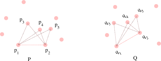
Figure 1: In this example, the rigid motion is obtained by matching $C_{Q}=\{q_{1},q_{2},\ldots,q_{5}\}$ in $Q$ to $C_{P}=\{p_{1},p_{2},\ldots,p_{5}\}$ in $P$. We have $\mathsf{LCP}(P,Q)=|C_{P}|=|C_{Q}|=5$. The corresponding 5-matching transformation $\mu$ can be discovered by matching $(q_{1},q_{2})$ to $(p_{1},p_{2})$, the rigid motions $\mu_{i}$ that transform $(q_{1},q_{2},q_{i})$ to $(p_{1},p_{2},p_{i})$ for $i=3,4,5$ are all the same and thus $\mu=\mu_{3}=\mu_{4}=\mu_{5}$ will get 3 votes, which is the maximum.

We call a key used to represent an ordered tuple $S$ a rigid motion invariant key if it satisfies the following: (1) the key remains the same for all $\mu(S)$ where $\mu$ is any rigid motion, and (2) for any two ordered tuples $S$ and $S^{\prime}$ with the same rigid motion invariant key there is a unique rigid motion $\mu$ such that $\mu(S)=S^{\prime}$. For example, as rigid motion preserves orientation and distances among points, given a non-degenerate triangle $\Delta$, the 3 side lengths of $\Delta$ together with the orientation (the sign of the determinant of the ordered triplet) form a rigid motion invariant key for $\Delta$ in $\mathbb{R}^{3}$. Henceforth, for simplicity of exposition, in the description of our algorithms we will omit the orientation part of the key.

2 Diheda

In this section, we introduce a new distance-approximation algorithm, called Diheda , for tolerant-LCP. The algorithm is based on a simple geometric observation. It can be seen as an improvement of a known GHT-based heuristic such that the output has theoretical guarantees.

2.1 Review of GHT

First, we review the idea of the pair-based version of GHT for exact-LCP. See the appendix or  [5, 31] for more details. For each congruent pair, say $(p_{1},p_{2})$ in $P$ and $(q_{1},q_{2})$ in $Q$, and for each of the remaining points $p\in P$ and $q\in Q$, if $(q_{1},q_{2},q)$ is congruent to $(p_{1},p_{2},p)$, compute the rigid motion $\mu$ that matches $(q_{1},q_{2},q)$ to $(p_{1},p_{2},p)$. We then cast one vote for $\mu$. The rigid motion that receives the maximum number of votes corresponds to the maximum matching transformation sought. See Figure 1 for an example.

2.2 Comparable rigid motions by dihedral angles

For the exact-LCP, one only needs to compare rigid motions by equality (for voting). For the tolerant-LCP, one needs to measure how close two rigid motions are. In $\mathbb{R}^{3}$, each rigid motion can be described by 6 parameters (3 for translations and 3 for rotations). How to define a distance measure between rigid motions? We will show below that the rigid motions considered in our algorithm are related to each other in a simple way that enables a natural notion of distance between the rigid motions.

Observation.

In the pair-based version of GHT as described above, the rigid motions to be compared have a special property: the rigid motions transform a common pair — they all match $(q_{1},q_{2})$ to $(p_{1},p_{2})$ in Figure 1. Two such transformations no longer differ in all 6 parameters but differ in only one parameter. To see this, we first recall that a dihedral angle is the angle between two intersecting planes; see Figure 2 for an example.

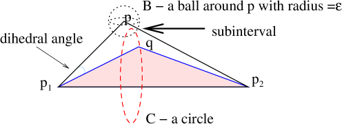
Figure 2: The dihedral angle is the angle between planes formed by $(p_{1},p_{2},q)$ and $(p_{1},p_{2},p)$. The rotation angles of transformations that rotate $q$ about $\stackrel{{\scriptstyle\longrightarrow}}{{p_{1}p_{2}}}$ to within $\epsilon$ of $p$ form a subinterval of $[0,2\pi)$.

In general, we can decompose the rigid motion for matching $(q_{1},q_{2},q_{3})$ to $(p_{1},p_{2},p_{3})$ into two parts: first, we transform $(q_{1},q_{2})$ to $(p_{1},p_{2})$ by a transformation $\phi_{1}$; then we rotate the point $\phi_{1}(q_{3})$ about $\stackrel{{\scriptstyle\longrightarrow}}{{p_{1}p_{2}}}$ by an angle $\theta$, where $\theta$ is the dihedral angle between the planes $(p_{1},p_{2},p_{3})$ and $(\phi_{1}(q_{1}),\phi_{1}(q_{2}),\phi_{1}(q_{3}))$. This will bring $q_{3}$ to coincide with $p_{3}$. Thus, we have the following lemma:

Lemma 2.1

Let $(p_{1},p_{2},p_{3})$ and $(q_{1},q_{2},q_{3})$ be two congruent non-collinear triplets, and let $\phi_{1}$ be a rigid motion that takes $q_{i}$ to $p_{i}$ for $i=1,2$. Let $\phi_{2}$ be the rotation about $\stackrel{{\scriptstyle\longrightarrow}}{{p_{1}p_{2}}}$ by an angle $\theta$, where $\theta$ is the dihedral angle between the planes $(p_{1},p_{2},p_{3})$ and $(\phi_{1}(q_{1}),\phi_{1}(q_{2}),\phi_{1}(q_{3}))$. Then the unique rigid motion that takes $(p_{1},p_{2},p_{3})$ to $(q_{1},q_{2},q_{3})$ is equal to $\phi_{2}\circ\phi_{1}$.

We now state another lemma that will be useful in the description and proof of correctness of Diheda . Let $(p_{1},p_{2},p)$ and $q$ be four points as shown in Figure 2. Consider the rotations about $\stackrel{{\scriptstyle\longrightarrow}}{{p_{1}p_{2}}}$ that take $q$ to within $\epsilon$ of $p$. The rotation angles of these transformations form a subinterval of $[0,2\pi)$. This is because a circle $C$ (corresponding to the trajectory of $p$) intersects with the sphere $B$ (around $p$ with radius $\epsilon$) at at most two points (corresponding to a subinterval of $[0,2\pi)$), as shown in Figure 2. That is, we have the following lemma:

Lemma 2.2

Let $p_{1},p_{2},p,q\in\mathbb{R}^{3}$ be four points (not necessarily non-collinear), then the rotation angles of transformations that rotate $q$ about $\stackrel{{\scriptstyle\longrightarrow}}{{p_{1}p_{2}}}$ to within $\epsilon$ of $p$ form a subinterval of $[0,2\pi)$.

2.3 Approximating the optimal rigid motion by the “diametric” rigid motion

For a point set $S\subset\mathbb{R}^{3}$, we call a pair of points $\{p,q\}\in S^{2}$ diameter-pair if $||p-q||=\mathsf{diameter}{(S)}$. A rigid motion of $Q$ that takes $q_{1}$ to $p_{1}$ and $q_{2}$ on the line $p_{1}p_{2}$ and closest possible to $p_{2}$ is called a $(p_{1},p_{2},q_{1},q_{2})$-rigid motion. Based on an idea similar to the one behind Lemma 2.4 in Goodrich et al. [19], we have the following lemma:

Lemma 2.3

Let $\mu$ be a rigid motion such that each point of $\mu(S)$, where $S\subseteq Q$, is within distance $\epsilon$ of a point in $P$. Let $\{q_{1},q_{2}\}$ be a diameter-pair of $S$. Let $p_{i}\in P$ be the closest point to $\mu(q_{i})$ for $i=1,2.$ Then we have a $(p_{1},p_{2},q_{1},q_{2})$-rigid motion $\mu^{\prime}$ of $Q$ such that each point of $\mu^{\prime}(S)$ is within $4\epsilon$ of a point in $P$.

Proof Sketch. Translate $\mu(q_{1})$ to $p_{1}$; this translation shifts each point by at most $\epsilon$. Next, rotate about $p_{1}$ such that $\mu(q_{2})$ is closest to $p_{2}$ (which implies $\mu^{\prime}(q_{1}),\mu^{\prime}(q_{2})$ and $p_{2}$ are collinear). Since $\{q_{1},q_{2}\}$ is a diameter-pair, this rotation moves each point by at most $2\epsilon$. Thus, each point is at most $\epsilon+\epsilon+2\epsilon=4\epsilon$ from its matched point.        

2.4 Approximation algorithm for tolerant-LCP

We first describe the idea of our algorithm Diheda . Input is two point sets in $\mathbb{R}^{3}$, $P=\{p_{1},\ldots,p_{m}\}$ and $Q=\{q_{1},\ldots,q_{n}\}$ with $m\geq n$, and $\epsilon\geq 0$. Suppose that the optimal rigid motion $\mu_{0}$ was achieved by matching a set $I_{\mu_{0}}=\{q_{1},q_{2},\ldots,q_{k}\}\subseteq Q$ to $J_{\mu_{0}}=\{p_{1},p_{2},\ldots,p_{k}\}\subseteq P$. WLOG, assume that $\{q_{1},q_{2}\}$ is the diameter pair of $I_{\mu_{0}}$. Then by Lemma 2.3, there exists a $(p_{1},p_{2},q_{1},q_{2})$-rigid motion $\mu$ of $Q$ such that $\mu(I_{\mu_{0}})$ is within $4\epsilon$ of a point in $P$. Since we do not know the matched set, we do not know a diameter-pair for the matched set either. Therefore, we exhaustively go through each possible pair. Namely, for each pair $(q_{1},q_{2})\in Q$ and each pair $(p_{1},p_{2})\in P$, if they are approximately congruent then we find a $(p_{1},p_{2},q_{1},q_{2})$-rigid motion $\mu$ of $Q$ that matches as many remaining points as possible. Note that $(p_{1},p_{2},q_{1},q_{2})$-rigid motions are determined up to a rotation about the line $p_{1}p_{2}$. By Lemma 2.2, the rotation angles that bring $\mu(q_{i})$ to within $4\epsilon$ of $p_{i}$ form a subinterval of $[0,2\pi)$. And the number of non-empty intersection subintervals corresponds to the size of the matched set. Thus, to find $\mu$, for each pair $(p,q)\in P\setminus\{p_{1},p_{2}\}\times Q\setminus\{q_{1},q_{2}\}$, we compute the dihedral angle interval according to Lemma 2.2. The rigid motion $\mu$ sought corresponds to an angle $\phi$ that lies in the maximum number of dihedral intervals. The details of the algorithm are described in Algorithm 1.

Algorithm 1 Diheda

1:

2:procedure Preprocessing

3:

4:for each pair $(p_{1},p_{2})$ of $P$ do

5:

6:Compute and insert the key of $||p_{1}p_{2}||$ into a dictionary ${\cal{D}}_{1}$;

7:end for

8:

9:for each triplet $(p_{1},p_{2},p_{3})$ of $P$ do

10:

11:Compute and insert the rigid motion invariant key for $(p_{1},p_{2},p_{3})$ into a dictionary ${\cal{D}}_{2}$;

12:end for

13:end procedure

14:

15:procedure Recognition

16:

17:for each pair $(q_{1},q_{2})$ of ${Q\choose 2}$  do $\triangleright$ This can be reduced by the edge set of an expander of $Q$.

18:

19:if $[||q_{1}q_{2}||-2\epsilon,||q_{1}q_{2}||+2\epsilon]$ exists in ${\cal{D}}_{1}$ then

20:

21:Initialize an empty dictionary ${\cal{D}}_{3}$ of pairs;

22:

23:for each remaining point $q\in Q$ do

24:

25:Compute and search the range $[||q_{1}q_{2}||-2\epsilon,||q_{1}q_{2}||+2\epsilon]\times[||qq_{1}||-2\epsilon,||qq_{1}||+2\epsilon]\times[||qq_{2}||-2\epsilon,||qq_{2}||+2\epsilon]$ of $(q_{1},q_{2},q)$ in ${\cal{D}}_{2}$; $\triangleright$ e.g. using a kd-tree.

26:

27:for each entry $(p_{1},p_{2},p)$ found do

28:

29:If $(p_{1},p_{2})$ exists in ${\cal{D}}_{3}$, increase its vote; otherwise insert $(p_{1},p_{2})$ into ${\cal{D}}_{3}$ with one vote;

30:

31:Append the matched pair $(q,p)$ to the list associated with $(p_{1},p_{2})$;

32:end for

33:end for

34:end if$\triangleright$ Compute the maximum transformation that matches $(q_{1},q_{2})$ to $(p_{1},p_{2})$.

35:

36:for each pair $(p_{1},p_{2})$ in the dictionary ${\cal{D}}_{3}$ do

37:

38:Compute a transformation $\phi$ that brings $q_{1}$ to $p_{1}$ and $q_{2}$ closest to $p_{2}$;

39:

40:For each matched pair $(q,p)$ of the associated list of $(p_{1},p_{2})$, compute an interval of dihedral angles such that $\phi(q)$ is within $4\epsilon$ of $p$;

41:

42:Sort all the intervals of dihedral angles; and find a dihedral angle $\psi$ that occurs in the largest number $V$ of intervals;

43:

44:Compute the transformation $\mu$ by the composition of $\phi$ and the rotation about $p_{1}p_{2}$ by angle $\psi$; $\triangleright$ $\mu$ brings $V+2$ points of $Q$ to within $4\epsilon$ of some matched points in $P$.

45:

46:Keep the maximum matched set size and the corresponding transformation;

47:end for

48:end for

49:end procedure

Time Complexity. For each triplet in $Q$, using kd-tree for range query, it takes $O(m^{3\cdot(1-\frac{1}{3})}+m^{3}+m^{3}\log{m^{2}})=O(m^{3}\log{m})$ for lines 11–20. For each pair $(q_{1},q_{2})$ and $(p_{1},p_{2})$, we spend time $O(mn)$ to find the subintervals for the dihedral angles, and time $O(mn\log{m})$ to sort these subintervals and do the scan to find an angle that lies in the maximum number of subintervals. Thus the total time is $O(m^{3}n^{3}\log{m})$.

3 Improvement by pigeonhole principle

In this section we show how a simple deterministic sampling strategy based on the pigeonhole principle yields speed-ups for the four basic algorithms for exact-$\alpha$-LCP. Specifically, we get a linear speed-up for pose clustering and GHT, and quadratic speed-up for alignment and geometric hashing. It appears to have been erroneously concluded previously that no such improvements were possible deterministically [26].

In pose clustering or GHT, suppose we know a pair $(q_{1},q_{2})$ in $Q$ that is in the sought matched set, then the transformation sought will be the one receiving the maximum number of votes among the transformations computed for $(q_{1},q_{2})$. Thus if we have chosen a pair $(q_{1},q_{2})$ that lies in the matched set, then the maximum matching transformation will be found. We are interested in the question “can we find a pair in the matched set without exhaustive enumeration”? The answer is yes: we only need to try a linear number of pairs $(q_{1},q_{2})$ to find the maximum matching transformation or conclude that there is none that matches at least $\frac{n}{\alpha}$ points.

We are given a set $Q=\{q_{1},\ldots,q_{n}\}$, and let $I\subseteq Q$ be an unknown set of size $\geq\frac{n}{\alpha}$ for some constant $\alpha>1$. We need to discover a pair $(p,q)$ with $p,q\in I$ by using queries of the following type. A query consist of a pair $(a,b)$ with $a,b\in Q$. If we have $a,b\in I$, the answer to the query is YES, otherwise the answer is NO. Thus our goal is to devise a deterministic query scheme such that as few queries are needed as possible in the worst case (over the choice of $I$) before a query is answered YES. Similarly, one can ask the question about querying triplets to discover a triplet entirely in $I$.

Theorem 3.1

For an unknown set $I\subseteq Q$ with $|I|\geq\frac{n}{\alpha}$ and $|Q|=n$ using queries as described above,

(1) it suffices to query $O(\alpha n)$ pairs to discover a pair in $I$;

(2) it suffices to query $O(\alpha^{2}n)$ triplets to discover a triplet in $I$.

Proof.  The proof is based on the pigeonhole principle. To prove (1), we assume for simplicity that $\alpha$ and $n\over\alpha$ are both integers. Partition the set $Q$ into $\frac{n}{\alpha}$ subsets of size $\alpha$ each. Since the size of $I$ is more than $\frac{n}{\alpha}$, by the pigeonhole principle, there is a pair of points in $I$ that lies in one of the above chosen subsets. Thus querying all pairs in these subsets will discover $I$. This gives that $\frac{n}{\alpha}{\alpha\choose 2}\sim\alpha n$ queries are sufficient to discover $I$.

Similarly, to prove (2), partition $Q$ into $n\over{2\alpha}$ subsets $P_{1},\ldots,P_{n\over{2\alpha}}$ of size $2\alpha$ each (we assume, as before, that $2\alpha$ and $n\over{2\alpha}$ are both integers). Now we test all triplets that lie in the $P_{i}$’s. Any set $I\subseteq Q$ that intersects with each of the $P_{i}$’s in at most $2$ points has size $\leq{n\over\alpha}$. Hence if $|I|>{n\over\alpha}$ then it must intersect with one of the sets above in at least $3$ points. Thus testing the triplets from the $P_{i}$’s is sufficient to discover $I$. The number of triplets tested is $\frac{n}{2\alpha}{2\alpha\choose 3}\sim\alpha^{2}n$.        

Remark: It can be shown that the schemes in the proof above are the best possible in requiring the smallest number of queries (up to constant factors).

In alignment and geometric hashing algorithms if we have chosen a triplet $(q_{1},q_{2},q_{3})$ from the maximum matching set $I\subseteq Q$ then we will discover $I$. The question, as before, is how many triplets in $Q$ need to be queried to discover a set $I$ of size $>{n\over\alpha}$. By Theorem 3.1 (2), we only need to query $O(\alpha^{2}n)$ triplets. Thus the running times of both alignment and geometric hashing are improved by a factor of $\Theta(n^{2})$.

See Table 1 for the time complexity comparison of deterministic algorithms for exact-$\alpha$-LCP in $\mathbb{R}^{3}$.

Finally, our approximation algorithm for tolerant-LCP adapts naturally for exact-$\alpha$-LCP with pigeonhole sampling. We analyze the running time of our algorithm for exact-$\alpha$-LCP with the pigeonhole sampling of pairs. In the exact case, each exact matched pair of points $(q,p)$ corresponds to a single dihedral angle. We thus find the dihedral angle that occurs the maximum number of times by sorting all the dihedral angles. For a fixed pair $(q_{1},q_{2})$ and a point $q$ in $Q$ the number of triplets $((p_{1},p_{2}),p_{3})$ in $P$ that match $((q_{1},q_{2}),q_{3})$ is bounded above by $3H_{2}(m)$, where $H_{2}(m)$ is the maximum possible number of the congruent triangles in a point set of size $m$ in $R^{3}$. Total time spent for pair $(q_{1},q_{2})$ then is $O(nH_{2})$. Since we use $O(\alpha n)$ pairs, the overall running time is $O(\alpha n^{2}H_{2})$. Agarwal and Sharir [1] show that $H_{2}(m)\leq m^{5\over 3}g(m)$, where $g(m)$ is a very slowly growing function of $m$ of inverse-Ackermann type.

Algorithm	Original running time	Improved running time
Pose Clustering (e.g. [31])	$O(m^{3}n^{3}S(m))$	$O(m^{3}n^{2}S(m))$
Alignment (e.g. [5])	$O(m^{3}+m\lambda^{3,2}(m,n))S(m)$	$O(m^{3}n^{2}S(m))$
GHT (e.g. [5])	$O(m^{3}S(m)+\lambda^{3,2}(m,n)S(\lambda^{3,2}(m,n)))$	$O(m^{3}S(m)+n^{2}H_{2}(m))$
Geometric hashing (e.g. [30])	$O(m^{4}S(m)+n^{4}H_{3}(m))$	$O(m^{4}S(m)+n^{2}H_{3}(m))$
This paper		$O(m^{3}S(m)+n^{2}H_{2}(m))$

Table 1: Time complexity comparison of deterministic algorithms for exact-$\alpha$-LCP in $\mathbb{R}^{3}$. $S(x)$ is the query time for the dictionary of size $x$, which can be taken to be $O(\log x)$ or smaller; $H_{2}(m)$ is the maximum number of triangles spanned by $m$ points in $\mathbb{R}^{3}$ that are congruent to a given triangle, we have $H_{2}(m)\leq m^{5\over 3}g(m)$, where $g(m)$ is a very slowly growing inverse-Ackermann type function of $m$ [1], and can be treated as constant for all practical purposes; $H_{3}(m)$ is the maximum number of tetrahedrons spanned by $n$ points in $\mathbb{R}^{3}$ that are congruent to a given tetrahedron, we have $H_{3}(m)=O(m^{2+\delta})$ for any $\delta>0$ [1]; $\lambda^{3,2}(m,n)=\tilde{O}(\min\{m^{1.8}n^{3},m^{1.95}n^{2.68}+m^{1.8875}n^{2.8}\})$[5].

As is often the case for algorithms for LCP, analysis involves determining quantities such as $H_{2}(m)$, which is a difficult problem. In the above table we have tried to give references for the first four algorithms including the tightest analyses rather than the original sources. Note that our algorithm is simpler than the others in the first column which involve checking for congruent simplices in a dictionary.

4 Expander-based sampling

While for the exact-$\alpha$-LCP the simple pigeonhole sampling served us well, for the tolerant-$\alpha$-LCP we do not know any such simple scheme for choosing pairs. The reason is that now we not only need to guarantee that each large set contain some sampled pairs, but also that each large set contain a sampled pair with large length (diameter-pair) as needed for the application of Lemma 2.3 in the Diheda algorithm. Our approach is based on expander graphs (see, e.g., [3]). Informally, expander graphs have linear number of edges but the edges are “well-spread” in the sense that there is an edge between any two sufficiently large disjoint subsets of vertices. Let $G$ be an expander graph with $Q$ as its vertex set. We show that for each $S\subseteq Q$, if $|S|$ is not too small, then there is an edge $(u,v)$ in $G$ such that $(u,v)\in S^{2}$ and $||uv||$ approximates the diameter of $S$.

By choosing the pairs for the Diheda algorithm from the edge set of $G$ (the rest of the algorithm is same as before), we obtain a bicriteria – distance and size – approximation algorithm as stated in Theorem 4.4 below. We first give a few definitions and recall a result about expander graphs that we will need to prove the correctness of our algorithm.

Definition 4.1

Let $S$ be a finite set of points of $\mathbb{R}^{r}$ for $r\geq 1$, and let $0\leq k\leq n$. Define $\mathsf{diameter}(S,k)=\min_{T:|T|=k}\mathsf{diameter}(S\setminus T).$

That is, $\mathsf{diameter}(S,k)$ is the minimum of the diameter of the sets obtained by deleting $k$ points from $S$. Clearly, $\mathsf{diameter}(S,0)=\mathsf{diameter}(S)$.

Let $U$ and $V$ be two disjoint subsets of vertices of a graph $G$. Denote by $e(U,V)$ the set of edges in $G$ with one end in $U$ and the other in $V$. We will make use of the following well-known theorem about the eigenvalues of graphs (see, e.g. [29], for the proof and related background).

Theorem 4.2

Let $G$ be a $d$-regular graph on $n$ vertices. Let $d=\lambda_{1}\geq\lambda_{2}\geq\ldots\geq\lambda_{n}$ be the eigenvalues of the adjacency matrix of $G$. Denote $\lambda=\max_{2\leq i\leq n}|\lambda_{i}|.$ Then for every two disjoint subsets $U,W\subset V$,

$$\left||e(U,W)|-\frac{d|U||W|}{n}\right|\leq\lambda\sqrt{|U||W|}.$$ (1)

Corollary 4.3

Let $U,W\subset V$ be two disjoint sets with $|U|=|W|>\frac{\lambda n}{d}$. Then $G$ has an edge in $U\times W$.

Proof.  It follows from (1) that if $\frac{d|U||W|}{n}>\lambda\sqrt{|U||W|}$ then $|e(U,W)|>0$, and since $|e(U,W)|$ is integral, $|e(U,W)|\geq 1$. But the above condition is clearly true if we take $U$ and $W$ as in the statement of Corollary 4.3.        

There are efficient constructions of graph families known with $\lambda<2\sqrt{d}$ (see, e.g., [3]). Let us call such graphs good expander graphs. We can now state our main result for this section.

Theorem 4.4

For an $\alpha$-LCP instance $(P,Q)$ with $\mathsf{LCP}(P,Q)>\frac{n}{\alpha}$, the Diheda algorithm with expander-based sampling using a good expander graph of degree $d>2500\alpha^{2}$ finds a rigid motion $\mu$ in time $O(m^{3}n^{2}\log{m})$ such that there is a subset $I$ satisfying the following criteria:

(1) size-approximation criterion: $|I|\geq\mathsf{LCP}(P,Q)-\frac{50}{\sqrt{d}}n$;

(2) distance-approximation criterion: each point of $\mu(I)$ is within distance $6\epsilon$ from a point in $P$.

Thus by choosing $d$ large enough we can get as good size-approximation as desired. The constants in the above theorem have been chosen for simplicity of the proof and can be improved slightly.

For the proof we first need a lemma showing that choosing the query pairs from a graph with small $\lambda(G)$ (the second largest eigenvalue of $G$) gives a long (in a well-defined sense) edge in every not too small subset of vertices.

Lemma 4.5

Let $G$ be a $d$-regular graph with vertex set $Q\subset\mathbb{R}^{3}$, and $|Q|=n$. Let $S\subseteq Q$ be such that $|S|>\frac{25\lambda(G)n}{d}$. Then there is an edge $\{s_{1},s_{2}\}\in E(G)\cap S^{2}$ such that $||s_{1}s_{2}||\geq{\mathsf{diameter}(S,\frac{25\lambda(G)}{d}n)\over 2}$.

Proof.  For a positive constant $c$ to be chosen later, remove $cn$ pairs from $S$ as follows. First remove a diameter pair, then from the remaining points remove a diameter pair, and so on. Let $T$ be the set of points in the removed pairs and $T^{p}$ the set of removed pairs. The remaining set $S\setminus T$ has diameter $\geq\mathsf{diameter}(S,2cn)$ by the definition of $\mathsf{diameter}(S,2cn)$, and hence each of the removed pairs has length $\geq\mathsf{diameter}(S,2cn)$. For $B,C\subset S$ let $||B,C||=\min_{b\in B,c\in C}||bc||$.

Claim 1

The set $T$ defined above can be partitioned into three sets $B$, $C$, $E$, such that $|B|,|C|\geq\frac{cn}{6}$, and $||B,C||\geq{\mathsf{diameter}(S,2cn)\over 2}$.

Proof.  Fix a Cartesian coordinate system and consider the projections of the pairs in $T^{p}$ on the $x$-, $y$- ,and $z$-axes. It is easy to see that for at least one of these axes, at least $cn\over 3$ pairs have projections of length $\geq{\mathsf{diameter}(S,2cn)\over\sqrt{3}}$. Suppose without loss of generality that this is the case for the $x$-axis, and denote the set of projections of pairs on the $x$-axis with length $\geq{\mathsf{diameter}(S,2cn)\over\sqrt{3}}$ by $T_{x}^{p}$, and the set of points in the pairs in $T_{x}^{p}$ by $T_{x}$. We have $|T_{x}|\geq 2cn/3$. Now consider a sliding window $W$ on the $x$-axis of length ${\mathsf{diameter}(S,2cn)\over 2}$, initially at $-\infty$, and slide it to $+\infty$. At any position of $W$, each pair in $T_{x}^{p}$ has at most $1$ point in $W$, as the length of any pair is more than the length of $W$. Thus at any position, $W$ contains $\leq{|T_{x}^{p}|}=|T_{x}|/2$ points. It is now easy to see by a standard continuity argument that there is a position of $W$, call it $\bar{W}$, where there are $\geq{|T_{x}|\over 4}\geq{cn\over 6}$ points of $T_{x}$ both to the left and to the right of $\bar{W}$.

Now, $B$ is defined to be the set of points in $T$ whose projection is in $T_{x}$ and is to the left of $\bar{W}$; similarly $C$ is the set of points in $T$ whose projection is in $T_{x}$ and is to the right of $\bar{W}$. Clearly any two points, one from $B$ and the other from $C$, are ${\mathsf{diameter}(S,2cn)\over 2}$-apart.        

Coming back to the proof of Lemma 4.5, the property that we need from the query-graph is that for any two disjoint sets $B,C\subset S$ of size $\delta|S|$, where $\delta$ is a small positive constant, the query-graph should have an edge in $B\times C$.

By Corollary 4.3 if $|B|\geq{cn\over 6}>\frac{\lambda n}{d}$, and $|C|\geq{cn\over 6}>\frac{\lambda n}{d}$, that is, if $c>{6\lambda\over d}$, then $G$ has an edge in $B\times C$. Taking $c=\frac{12.5\lambda}{d}$ completes the proof of Lemma 4.5.        

Proof of Theorem 4.4. If we take $G$ to be a good expander graph then Lemma 4.5 gives that $G$ has an edge of length $\geq{\mathsf{diameter}(S,\frac{50}{\sqrt{d}}n)\over 2}$. Let $S$ also be a solution to tolerant-LCP for input $(P,Q)$ with error parameter $\epsilon>0$. We have that one of the sampled pairs has length at least ${\mathsf{diameter}(S,\frac{50}{\sqrt{d}}n)\over 2}$. Thus applying an appropriate variant (replacing the diameter pair by the sampled pair with large length as guaranteed by Lemma 4.5) of Lemma 2.3, we get a rigid motion $\mu$ such that there is a subset $I$ satisfying the following:

(1) $|I|\geq|S|-\frac{50}{\sqrt{d}}n$ for any $d>2500\alpha^{2}$;

(2) Each point of $I$ is within $6\epsilon(=\epsilon+\epsilon+4\epsilon)$ of a point in $M$.        

5 Discussion

We have presented a new practical algorithm for point pattern matching. Our Diheda algorithm is the fastest known distance-approximation algorithm for tolerant-LCP, and is simple compared to other known distance-approximation algorithms and heuristics which involve 6-dimensional clustering. Our analysis of Diheda is not tight, and perhaps better bounds can be obtained if the interpoint distance is greater than $\epsilon$ by a sufficiently large constant factor.

Our technique of pigeonhole sampling yields speed-ups for all four popular algorithms and also the fastest known deterministic algorithm for the exact-LCP. Again, our algorithms are simpler than the previous best algorithms. Akutsu et al. [5] give a tighter analysis for GHT in terms of the function $\lambda^{3,2}(m,n)$. Our analysis of Diheda (and GHT) with pigeonhole sampling was based on $H_{2}(m)$. Presumably, a better analysis similar to the idea in [5] is possible.

Point pattern matching is of fundamental importance for computer vision and structural bioinformatics. Indeed, this investigation stemmed from research in structural bioinformatics. Current software, which uses either geometric hashing or generalized Hough transform, can immediately benefit from this work. We have implemented a randomized version of Diheda for molecular common substructure detection and the results were reported in  [16].

Acknowledgment. We thank S. Muthukrishnan and Ali Shokoufandeh for the helpful comments and advice.

Appendix

Appendix A Voting Algorithms for Exact-LCP

In this appendix, we review and compare four popular algorithms for exact-LCP: pose clustering, alignment, generalized Hough transform(GHT), and geometric hashing. These algorithms are all based on a voting idea and are sometimes confused in the literature. Please see Algorithms 2, 3, 4, 5) for a full description of the algorithms in their generic form independent of the search data structure used. In particular, geometric hashing algorithms need not use a hash-table as a search data structure. We describe all the algorithms in terms of a dictionary of objects (which are either transformations or a set of points and can be ordered lexicographically). Denote the query time for this dictionary by $S(x)+O(k)$ where $x$ is the size of the dictionary, and $k$ is the size of the output depending on the query. For example, if the dictionary is implemented by a search tree we have $S(x)=O(\log x)$.

Pose clustering and alignment are the basic methods. GHT and geometric hashing can be regarded as their respective efficient implementations. Efficiency is achieved by preprocessing of the point sets using their rigid motion invariant keys which speeds-up the searches.

In pose clustering, for each pair of triplets $(q_{1},q_{2},q_{3})\in Q$ and $(p_{1},p_{2},p_{3})\in P$, we check if they are congruent. If they are then we compute the rigid motion $\mu$ such that $\mu(q_{1},q_{2},q_{3})=(p_{1},p_{2},p_{3})$. We then cast one vote for $\mu$. The rigid motion which receives the maximum number of votes corresponds to the maximum matching transformation sought. The running time of pose clustering is $O(m^{3}n^{3}S(m^{3}n^{3}))$ as the size of the dictionary of transformations can be as large as $O(m^{3}n^{3})$.

In alignment, for each pair of triplets $(q_{1},q_{2},q_{3})\in Q$ and $(p_{1},p_{2},p_{3})\in P$ we check if they are congruent. If they are then we compute the rigid motion $\mu$ such that $\mu(q_{1},q_{2},q_{3})=(p_{1},p_{2},p_{3})$. Then we count the number of points in $\mu(Q)$ that coincide with points in $P$. This number gives the number of votes the rigid motion $\mu$ gets. The rigid motion which receives the maximum number of votes corresponds to the maximum matching transformation sought. The running time is $O(m^{3}n^{4}S(m))$.

The difference between pose clustering and alignment is the voting space: in pose clustering voting is done for transformations while in alignment it is for bases (triplets of points). In both pose clustering and alignment algorithms, each possible triplet in $Q$ is compared with each possible triplet in $P$. However, by representing each triplet with its rigid motion invariant key, only triplets with the same key (rigid motion invariant) are needed to be compared. This provides an efficient implementation. For example, the GHT algorithm is an efficient implementation of pose clustering. Here we preprocess $P$ by storing the triplets of points with the rigid motion invariant keys in a dictionary. Now for each triplet $(q_{1},q_{2},q_{3})$ in $Q$ we find congruent triplets in $P$ by searching for the rigid motion invariant key for $(q_{1},q_{2},q_{3})$. The rest of the algorithm is the same as pose clustering. Similarly the geometric hashing algorithm is an efficient implementation of the alignment method.

GHT is faster than geometric hashing, however geometric hashing has the advantage that algorithm can stop as soon as it has found a good match. Depending on the application this gives geometric hashing advantage over GHT.

As observed by Olson [31] and Akutsu et al. [5], pose clustering and GHT can be further improved. This is because a $k$-matching transformation can be identified by matching $(k-2)$ bases which match a common pair. We call this version of the generalized Hough transform the pair-based version; it is described below in Algorithm 6. Although the worst case time complexity of the pair-based version and the original version are the same, this will serve as a basis for our new scheme, called Diheda . The pair-based version also allows efficient random sampling of pairs [31, 5].

Algorithm 2 Pose Clustering

1:

2:procedure Pose Clustering($P,Q$)

3:

4:Initialize an empty dictionary $\cal{D}$ of rigid motions;

5:

6:for each triplet $(q_{1},q_{2},q_{3})$ of $Q$ do

7:

8:for each triplet $(p_{1},p_{2},p_{3})$ of $P$ do

9:

10:if $(q_{1},q_{2},q_{3})$ is congruent to $(p_{1},p_{2},p_{3})$, then

11:

12:Compute the rigid motion $\mu$ which matches $(q_{1},q_{2},q_{3})$ to $(p_{1},p_{2},p_{3})$ ;

13:

14:Search $\mu$ in the dictionary $\cal{D}$;

15:

16:If found, increase the votes of $\mu$; otherwise insert $\mu$ with one vote.

17:end if

18:end for

19:end for

20:

21:Return the maximum vote rigid motion in $\cal{D}$;

22:end procedure

Algorithm 3 Alignment

1:

2:procedure Alignment($P,Q$)

3:

4:for each triplet $(q_{1},q_{2},q_{3})$ of $Q$ do

5:

6:for each triplet $(p_{1},p_{2},p_{3})$ of $P$ do

7:

8:If $(q_{1},q_{2},q_{3})$ is congruent to $(p_{1},p_{2},p_{3})$, compute the rigid motion $\mu$;

9:

10:Vote = 0; $\triangleright$ Vote is a local counter for the transformation $\mu$.

11:

12:for each remaining point $q\in Q$ and $p\in P$  do

13:

14:If $\mu(q)=p$, then increase Vote by 1;

15:end for

16:

17:Keep the maximum vote and its associated transformation;

18:end for

19:end for

20:

21:Return the maximum vote transformation.

22:end procedure

Algorithm 4 The original version of generalized Hough transform.

1:

2:procedure Preprocessing

3:

4:for each triplet $(p_{1},p_{2},p_{3})$ of $P$ do

5:

6:Compute and insert the rigid motion invariant key for $(p_{1},p_{2},p_{3})$ into a dictionary ${\cal{D}}_{1}$;

7:end for

8:end procedure

9:

10:procedure Recognition

11:

12:Initialize an empty dictionary ${\cal{D}}_{2}$ of rigid motions;

13:

14:for each triplet $(q_{1},q_{2},q_{3})$ of $Q$ do

15:

16:Compute and search the rigid motion invariant key for $(q_{1},q_{2},q_{3})$ in the dictionary ${\cal{D}}_{1}$;

17:

18:for each entry $(p_{1},p_{2},p_{3})$ found, do

19:

20:Compute the rigid motion $\mu$ which matches $(q_{1},q_{2},q_{3})$ to $(p_{1},p_{2},p_{3})$;

21:

22:Search $\mu$ in the dictionary ${\cal{D}}_{2}$;

23:

24:If found, increase the votes of $\mu$; otherwise insert $\mu$ with one vote into ${\cal{D}}_{2}$;

25:end for

26:end for

27:

28:Return the maximum vote rigid motion in ${\cal{D}}_{2}$;

29:end procedure

Algorithm 5 Geometric Hashing

1:

2:procedure Preprocessing

3:

4:for each triplet $(p_{1},p_{2},p_{3})$ of $P$ do

5:

6:for each of the remaining point $p$ of $P$ do

7:

8:Compute and insert the rigid motion invariant key for $\{(p_{1},p_{2},p_{3}),p\}$ into a dictionary ${\cal{D}}_{1}$;

9:end for

10:end for

11:end procedure

12:

13:procedure Recognition

14:

15:for each triplet $(q_{1},q_{2},q_{3})$ of $Q$ do

16:

17:Build an empty dictionary ${\cal{D}}_{2}$ (of triplets of $P$);

18:

19:for each of the remaining point $q$ of $Q$ do

20:

21:Compute and search the rigid motion invariant key for $\{(q_{1},q_{2},q_{3}),q\}$ in the dictionary ${\cal{D}}_{1}$;

22:

23:for each entry $\{(p_{1},p_{2},p_{3}),p\}$ found do

24:

25:If $(p_{1},p_{2},p_{3})$ exists in ${\cal{D}}_{2}$, then increase its vote by one; otherwise insert $(p_{1},p_{2},p_{3})$ into ${\cal{D}}_{2}$ with vote one.

26:end for

27:end for

28:

29:Keep the maximum vote and compute the corresponding transformation from its associated triplet;

30:end for

31:end procedure

Algorithm 6 The pair-based version of generalized Hough transform.

1:

2:procedure Preprocessing

3:

4:for each pair $(p_{1},p_{2})$ of $P$ do

5:

6:for each remaining point $p$ of $P$ do

7:

8:Compute and insert the rigid motion invariant key for $\{(p_{1},p_{2}),p\}$ into a dictionary $\cal{D}$;

9:end for

10:end for

11:end procedure

12:

13:procedure Recognition

14:

15:for each pair $(q_{1},q_{2})$ of $Q$ do

16:

17:Initialize an empty dictionary ${\cal{D}}_{2}$ of rigid motions;

18:

19:for each remaining point $q$ of $Q$ do

20:

21:Compute and search the rigid motion invariant key for $\{(q_{1},q_{2}),q\}$ in the dictionary $\cal{D}$;

22:

23:for each entry $\{(p_{1},p_{2}),p\}$ found, do

24:

25:Compute the rigid motion $\mu$ which matches $\{(q_{1},q_{2}),q\}$ to $\{(p_{1},p_{2}),p\}$.

26:

27:Search $\mu$ in the dictionary ${\cal{D}}_{2}$;

28:

29:If found, increase the votes of $\mu$; otherwise insert $\mu$ with one vote into ${\cal{D}}_{2}$;

30:end for

31:end for

32:

33:Keep the rigid motion for $(q_{1},q_{2})$ that receives the maximum number of votes.

34:end for

35:

36:Return the rigid motion that receives the maximum number of votes among all pairs.

37:end procedure

References

- [1] P. K. Agarwal and M. Sharir, The number of congruent simplices in a point set, Discrete Comput. Geom. 28 no. 2 (2002) 123–150.
- [2] M. Ajtai, N. Megiddo, A Deterministic Poly(log log N)-Time N-Processor Algorithm for Linear Programming in Fixed Dimension, in: Proc. 24th ACM Symp. on Theory of Computing (1992), 327–338.
- [3] N. Alon and J. Spencer, The Probabilistic Method, (Wiley-Interscience, 2000)
- [4] T. Akutsu, Protein structure alignment using dynamic programming and iterative improvement, IEICE Transactions on Information and Systems 12 (1996) 1629–1636.
- [5] T. Akutsu, H. Tamaki, T. Tokuyama, Distribution of Distances and Triangles in a Point Set and Algorithms for Computing the Largest Common Point Sets, Discrete & Computational Geometry 20 no.3 (1998) 307–331.
- [6] T. Akutsu, K. Kanaya, A. Ohyama, A. Fujiyama, Point matching under non-uniform distortion, Discrete Applied Mathematics, 127(1) (2003) 5–21.
- [7] H. Alt and L.J. Guibas, Discrete Geometric Shapes: Matching, Interpolation, and Approximation, in: J.-R. Sack, J. Urrutia, eds., Handbook of Computational Geometry, (Elsevier Science Publishers B.V. North-Holland, Amsterdam, 1999) 121–153.
- [8] H. Alt, K. Mehlhorn, H. Wagener, E. Welzl, Congruence, Similarity, and Symmetries of Geometric Objects, Discrete & Computational Geometry 3 (1988) 237–256.
- [9] C. Ambühl, S. Chakraborty, B. Gärtner. Computing Largest Common Point Sets under Approximate Congruence. ESA 2000, Lecture Notes in Computer Science 1879 Springer 2000: 52–63.
- [10] S. Biswas, S. Chakraborty. Fast Algorithms for Determining Protein Structure Similarity. Workshop on Bioinformatics and Computational Biology, at the International Conference on High Performance Computing (HiPC), Hyderabad, India, December 2001.
- [11] S. Chakraborty, S. Biswas. Approximation Algorithms for 3-D Commom Substructure Identification in Drug and Protein Molecules. Workshop on Algorithms and Data Structures (WADS), 1999. Lecture Notes in Computer Science 1663.
- [12] D. Cardoze, L. Schulman. Pattern Matching for Spatial Point Sets. Proc. 39th FOCS 156–165, 1998.
- [13] L.P. Chew, D. Dor, A. Efrat and K. Kedem. Geometric Pattern Matching in d-Dimensional Space, Discrete and Computational Geometry, 21(1999), pp. 257-274.
- [14] V. Choi, N. Goyal. A Combinatorial Shape Matching Algorithm for Rigid Protein Docking. Combinatorial Pattern Matching (CPM) 2004 Lecture Notes in Computer Science 3109 Springer 2004: 285-296.
- [15] V. Choi, N. Goyal. An Efficient Approximation Algorithm for Point Pattern Matching Under Noise. The 7th International Symposium, Latin American Theoretical Informatics (LATIN 2006). Valdivia, Chile, March 19–24, 2006. Lecture Notes in Computer Science, Vol. 3887, 2006, pp 298–310.
- [16] V. Choi, N. Goyal. An Algorithmic Approach to the Identification of Rigid Domains in Proteins. Submitted to Algorithmica’s special issue on algorithms for processing protein structures.
- [17] P. Finn, L. Kavraki, J-C. Latombe, R. Motwani, C. Shelton, S. Venkatasubramanian, A. Yao. RAPID: Randomized Pharmacophore Identification in Drug Design The 13th Symposium on Computational Geometry, 1997. Computational Geometry: Theory and Applications 10 (4), 1998.
- [18] M. Gavrilov, P. Indyk, R. Motwani, S. Venkatasubramanian. Combinatorial and Experimental Methods for Approximate Point Pattern Matching. Algorithmica 38(1): 59–90 (2003).
- [19] M. T. Goodrich, J. S. B. Mitchell, M. W. Orletsky. Approximate Geometric Pattern Matching Under Rigid Motions. IEEE Trans. Pattern Anal. Mach. Intell. 21(4): 371-379 (1999).
- [20] W. E. L. Grimson, D. P. Huttenlocher. On the sensitivity of geometric hashing. In Proceedings of the 3rd International Conference on Computer Vision: 334–338 (1990)
- [21] W. E. L. Grimson, D. P. Huttenlocher. On the sensitivity of Hough transform for object recognition. IEEE Trans. on Pattern Analysis and Machine Intell. 12(3): 1990.
- [22] Y. Hecker and R. Bolle. On geometric hashing and the generalized Hough transform. IEEE Trans. on Systems, Man and Cybernetics, 24, pp. 1328-1338, 1994
- [23] P. J. Heffernan, S. Schirra. Approximate Decision Algorithms for Point Set Congruence, Comput. Geom. 4 (1994) 137–156.
- [24] J. Hopcroft, R. Karp. An algorithm for maximum matchings in bipartite graphs. SIAM J. Comp. 2 (1973) 225–231.
- [25] P. Indyk, R. Motwani, S. Venkatasubramanian. Geometric Matching under Noise: Combinatorial Bounds and Algorithms. SODA, 1999.
- [26] S. Irani, P. Raghavan. Combinatorial and experimental results for randomized point matching algorithms. The 12th Symposium on Computational Geometry, 1996. Comput. Geom. 12(1-2): 17–31 (1999).
- [27] M. Katz, M. Sharir. An expander-based approach to geometric optimization. SIAM J. Comput., Vol. 26, No. 5, 1384–1408, 1997.
- [28] C. Kenyon, Y. Rabani, and A. Sinclair. Low Distortion Maps Between Point Sets. Proceedings of the Thirty-Sixth Annual ACM Symposium on Theory of Computing (STOC), 2004.
-
[29]
M. Krivelevich, B. Sudakov.
Pseudo-random graphs.
Preprint. Available at http://www.math.tau.ac.il/
~krivelev/papers.html - [30] Y. Lamdan, H. J. Wolfson. Geometric Hashing: A general and efficient model-based recognition scheme. In Second International Conference on Computer Vision, 238–249 (1988).
- [31] C. F. Olson. Efficient Pose Clustering Using a Randomized Algorithm. International Journal of Computer Vision 23(2), 131–147 (1997).
- [32] H. J. Wolfson and I. Rigoutsos. Geometric hashing: an overview. IEEE Computational Science and Engineering, Vol 4, 10–21 (1997).
- [33] R. Nussinov, H.J. Wolfson. Efficient Detection of Three - Dimensional Motifs In Biological Macromolecules by Computer Vision Techniques, Proc. of the Nat’l Academy of Sciences, 88 (1991) 10495 – 10499.