MODELLING INVESTMENT IN ARTIFICIAL STOCK MARKETS: ANALYTICAL AND NUMERICAL RESULTS

Abstract

In this article we study the behavior of a group of economic agents in the context of cooperative game theory, interacting according to rules based on the Potts Model with suitable modifications. Each agent can be thought of as belonging to a chain, where agents can only interact with their nearest neighbors (periodic boundary conditions are imposed). Each agent can invest an amount $\sigma_{i}=0,...,q-1$. Using the transfer matrix method we study analytically, among other things, the behavior of the investment as a function of a control parameter (denoted $\beta$) for the cases $q=2$ and $3$. For $q>3$ numerical evaluation of eigenvalues and high precision numerical derivatives are used in order to assess this information.

keywords: Game Theory; statistical mechanics; transfer matrix methods.

I Introduction

Consider a game where N players can invest their money (up to some upper limit) on some public–fund asset. The fund manager, as a rule, doubles the amount of money received and divides it equally among all N investors. Depending on the total amount each player invested, some might end up making a profit while others may lose money. Assume that players have no information whatsoever about their co-players’ moves. The question is: what is the best move a player can make? If we adopt one of the tenets of classical game theory, namely that players are completely rational, then there are two possible solutions to the problem which maximize profit (when all invest the maximum amount possible, thus doubling their initial capital) or minimize losses (no one invests anything). In the real world however people are not rational in the sense of classical game theory and factors as expectations about the behavior of other players or some sort of insider information might play a role when deciding how to invest.

The irrationality of market agents is one of a myriad of factors which account for the high complexity of financial markets and the difficulty in modelling them. Markets may also be affected by political turmoil, unseasonable weather variations and the like. In the past few years models have been introduced in order to throw some light into the behavior of markets, mainly with aims at forecasting long-term behavior see for example Br1993 ; Bl1993 . These models, which have the advantage of being either analytically or numerically treatable and usually use some kind of data input from real markets, are nonetheless unable to take into account the human factor in decision-making scenarios. To circumvent these difficulties a new approach, inspired on the ideias of statistical mechanics has been suggested D1999 , where one extends the set of causal factors in decision–making scenarios from the individual–specific to group determinants of behavior: players’ decisions are not market–mediated but rely on group–level influences.

With these ideias in mind our aim in this work is to extend the model for the game discussed above through the introduction of cooperation, i.e. we allow agents to have partial information on the decision of its immediate neighbors, in a way to be described precisely in what follows. Furthermore, we allow for some kind of randomness, the only thing known a priori being the probability of some decision, and not the decision itself. In this way we hope to describe the average behavior of a large group of agents without entering in the details of a realistic (and certainly very difficult) theory on psychological state of each agent.

Our main interest will be to see how is the average behavior of a (large) group of cooperative economic agents. Each agent, labelled by the index $i$, is allowed to invest an amount $\sigma_{i}$. Before the investment, the agent $i$ exchange information with agent $i+1$ (defined as the neighbor of $i$; this concept is symmetric, i.e., $i$ is also neighbor of $i+1$). Based on that information agents make decisions as to how much they will invest according to some probability distribution parameterized in terms of a two real variables: $J$ and $\beta$. The first measures how strongly people interact with each other (group–level influence) while the later is a measure of how strongly a player might deviate from the group. To model this we choose a suitably defined function which measures the probability of $i$ investing $\sigma_{i}$ given that $i+1$ would like to invest $\sigma_{i+1}$. In a way to be precisely formalized later, $\beta$ allows us to change the expected behavior of each agent.

The paper is organized as follows: In section $2$ we explain the model and make the connection with statistical mechanics. Using the standard transfer matrix techniqueH1987 we analyze in section $3$ some integrable cases ($q=2$ and $q=3$) in order to gain information about how the average investment changes as a function of $\beta$. In section $4$ we numerically evaluate the evolution for $q\geq 4$. We introduce a method for calculating the investment using derivatives of the biggest eigenvalue, which is based on the use of 5 points in a graphic. We finish the paper with some conclusions and perspectives.

II Formulating the problem: the Potts Model

We consider an ensemble of $N$ agents, where each can invest an amount $\sigma_{i}\in\{0,1,\dots,q-1\}$, $q$ a fixed integer. This restriction on $q$ has been made for the sake of clarity. The methods employed can be easily generalized to the case where $\sigma_{i}\in\{d_{0},\ldots,d_{q-1}\}$, the $d_{i}$’s being arbitrary real numbers.

The families of conditional probabilities, i.e. the probability that $i+1$ would invest $\sigma_{i+1}$ given that $i$ invested $\sigma_{i}$ are chosen as

$$P(\sigma_{i+1}|\sigma_{i})=c\exp\left[-\beta\cdot J(\sigma_{i})\cdot\delta_{\sigma_{i},\sigma_{i+1}}\right]\;.$$ (1)

Our motivation for this particular choice comes from physics, where this probability is interpreted as that of two variables (called classical spins) $\sigma_{i}$ and $\sigma_{i+1}$ being equal or having different values. It depends on two physical parameters: $J(\sigma_{i})$ is the so–called interaction strength. This is in most cases a material–dependent quantity and accounts for the different collective properties materials may exhibit (ferromagnetic, antiferromagnetic, etc.). $\beta$ is proportional to the inverse temperature $T^{-1}$ and brings about entropic effects (ordered states for low temperatures and disorder for high temperatures). Being proportional to a temperature, in physical systems $\beta$ is always non negative, and we likewise assume our $\beta\geq 0$.

In general $J$ and $\beta$ can be seen as competing terms: $J$ is associated to the energy cost of a given spin configuration. For $J>0$ ($<0$) a configuration where spins are equal (different) has a higher energy than the opposite configuration, which means that it is energetically more favorable to be non–magnetic (or ferromagnetic); on the other hand, the temperature $\beta^{-1}$ tends to destroy magnetic order. Transposing these ideas to the financial context can say that $J(\sigma_{i})$ measures how strongly people respond to their neighbors’ moves, that is if they are susceptible to the influence of other players or not. In this sense it models distinct profiles of investors, which can go from agressive (does not go along “with the pack”) to conservative (does what others do). $\beta$ is a measure of the strength of individual response and independent of what others do. Social scientists refer to this term as the “individual–specific random” and “unobservable” (from the point of view of the modeler) since it is associated to personal beliefs D1999 .

With the neighbor-to-neighbor interaction rule introduced above we can describe the behavior of the whole group: The first important quantity which needs to be defined is the joint probability density (j.p.d), $P(\sigma_{1},\sigma_{2},...,\sigma_{N})$ of a particular investment configuration $\sigma\equiv(\sigma_{1},\sigma_{2},...,\sigma_{N})$ of a group. The quantity invested is defined through

$$L(\sigma)=\sigma_{1}+\sigma_{2}+...+\sigma_{N}$$ (2)

and we would like to obtain the average value of $L$.

To calculate the j.p.d we may adopt a recursive formulation without any loss of generality: we take the investment of the first agent to be exactly $\sigma_{1}$, i.e., $P(\sigma_{1})=1$ and from that derive the quantity we want. With this “boundary condition” on $P(\sigma_{1})$ we have the following theorem:

Theorem 1

The probability distribution $P(\sigma_{1},\sigma_{2},...,\sigma_{N})$ can be written as a product form

$$P(\sigma_{1},\sigma_{2},...,\sigma_{N})=\prod\limits_{i=1}^{N-1}P(\sigma_{i+1}|\sigma_{i})$$ (3)

with $P(\sigma_{i}|\sigma_{i-1},...,\sigma_{1})=P(\sigma_{i}|\sigma_{i-1})$ for $i=1,...,N$.

Proof. ¿From the definition

$$P(\sigma_{N}|\sigma_{1},\sigma_{2},...,\sigma_{N-1})=\frac{P(\sigma_{1},\sigma_{2},...,\sigma_{N})}{P(\sigma_{1},\sigma_{2},...,\sigma_{N-1})}$$ (4)

Considering the hypothesis $P(\sigma_{N}|\sigma_{1},\sigma_{2},...,\sigma_{N-1})=P(\sigma_{N}|\sigma_{N-1})$ we thus have

$$P(\sigma_{1},\sigma_{2},...,\sigma_{N})=P(\sigma_{1},\sigma_{2},...,\sigma_{N-1})P(\sigma_{N+1}|\sigma_{N})\;.$$ (5)

and applying this recursively:

$$\begin{array}[]{lll}P(\sigma_{1},\sigma_{2},...,\sigma_{N})&=&P(\sigma_{1},\sigma_{2},...,\sigma_{N-1})P(\sigma_{N}|\sigma_{N-1})\\ &&\\ &=&P(\sigma_{1},\sigma_{2},...,\sigma_{N-2})P(\sigma_{N-1}|\sigma_{N-2})P(\sigma_{N}|\sigma_{N-1})\\ &&\\ &=&P(\sigma_{1})\prod\limits_{i=1}^{N-1}P(\sigma_{i+1}|\sigma_{i})=\prod\limits_{i=1}^{N-1}P(\sigma_{i+1}|\sigma_{i})\end{array}$$

   According to equations (1) and (3) we have

$$P(\sigma_{1},\sigma_{2},...,\sigma_{N})=c^{N}\exp\left[-\beta\sum_{i=1}^{N-1}J(\sigma_{i})\cdot\delta_{\sigma_{i},\sigma_{i+1}}\right]$$

where $c^{N}$ is the normalization constant defined before and such that

$$\sum\limits_{\sigma_{1}=d_{0}}^{d_{q-1}}\sum\limits_{\sigma_{2}=d_{0}}^{d_{q-1}}...\sum\limits_{\sigma_{N}=d_{0}}^{d_{q-1}}P(\sigma_{1},\sigma_{2},...,\sigma_{N})=1\qquad.$$

II.1 Investment formulas and the Potts model

The Potts hamiltonian of $N$ interacting spins under the action of a magnetic field $D$ is given by W1973

$$H\left(\sigma\right)=\sum\limits_{\left\langle i,j\right\rangle}J(\sigma_{i})\delta_{\sigma_{i},\sigma_{j}}+D\sum\limits_{i=1}^{N}\sigma_{i}.$$ (6)

The fact that the total investment $L$ (2) is mathematically the same as the magnetization of the Potts hamiltonian (6) means that we may directly transpose the techniques and ideas of statistical mechanics into the financial scenario.

The probability density function for the system to present a specific investment value $L$ is given by

$$P(L)=\left\{\begin{array}[]{lll}Z_{N}^{-1}\exp\left[-\beta H(\sigma)\right]&\;\;\;\;\;{\mbox{if}}&\;\;L=\sum\nolimits_{i=1}^{N}\sigma_{i}\\ &&\\ 0&{\mbox{otherwise}}&\end{array}\right.$$ (7)

where $Z_{N}(\beta)$, the normalization constant, is a sum over all possible configurations

$$Z_{N}(\beta)=\sum\limits_{\sigma_{j}=0,...,q-1}\exp\left[-\beta H\left(\sigma\right)\right].$$ (8)

and is known as the partition function.

Our aim is to describe how the investment depends on $\beta$, given a fixed set of parameters $J(1),J(2),...,J(N)$. For this purpose, let us consider the expected value of $L$ according to the distribution (7), i.e.

$$\left\langle L\left(\sigma\right)\right\rangle=\frac{1}{Z}\sum\limits_{\sigma_{j}=0,...,q-1}\left(\sum\limits_{i=1}^{N}\sigma_{i}\right)\exp\left[-\beta H\left(\sigma\right)\right].$$

For the sake of those not familiar with the methods of statistical mechanics, we briefly discuss how in our analogy between spin systems and economic games quantities of interest can be calculated:

1. The term $D\sum\limits_{i=1}^{N}\sigma_{i}$ is introduced for convenience since investment per capita is calculated through the formulae

   $$l(\beta)=\frac{1}{N}\left\langle L(\beta)\right\rangle=\left.-\frac{1}{\beta N}\frac{\partial}{\partial D}\log Z_{N}(\beta)\right|_{D=0},$$

   which is the analogue in statistical mechanics to the average spontaneous magnetization. It clearly obeys the inequality $0\leq l\leq q-1$.

2. As previously discussed, investment depends essentially on the way how neighbors cooperate, i.e. the distribution $J(0),J(1),...$.$J(q-1)$ defines the kind of profiles investors have.

The first question one might ask would be: what is the behavior of the per capita investment $l(\beta)$ at $\beta=0$ and $\beta\rightarrow\infty$ ? One may describe these limits in a straightforward manner:

Theorem 2

The per capita investment is such that

$l(0)=\frac{q-1}{2};$

$l(\infty)=\sigma_{min}$ if $J_{min}$ satisfies the inequality $J_{min}<J_{k}$ for all $k=0,\ldots,min-1,min+1,\ldots,q-1$.

Proof. The probability of a given state $\sigma=\left\{\sigma_{i}\right\}_{i=1}^{N}$ is

$$P(\sigma)=\frac{e^{-\beta H(\sigma)}}{Z_{N}(\beta)};$$

For $\beta=0$ all states are equiprobable since, from the equation above, the probability does not depend on $\sigma$; hence, the probability of each state is $1/q^{N}$. For simplicity we assume that $q^{N}$ is even, the odd case being left to the reader. The per capita investment can be written as

$$l(0)=\frac{1}{Nq^{N}}\sum_{i=0}^{N(q-1)}(\mbox{number of states with sum $=i$})i$$

We can see that the number of states corresponding to the sum $i$ is the same as the number corresponding to the sum $N(q-1)-i$. Then,

$$l(0)=\frac{1}{Nq^{N}}\sum_{i=0}^{N(q-1)/2}(\mbox{number of states with sum $=i$})N(q-1)=$$

$$\frac{1}{Nq^{N}}N(q-1)\frac{q^{N}}{2}=\frac{q-1}{2}$$

since the number of states with sum between $0$ and $N(q-1)/2$ correspond to $(q^{N})/2$.

For arbitrary values of $\beta$ let us call $\sigma_{M}=\left\{\sigma_{min}\right\}_{i=1}^{N}$. Then, the probability of any state is

$$P(\sigma)=\frac{e^{-\beta H(\sigma)}}{e^{-\beta H(\sigma_{M})}\left(1+\sum\nolimits_{\sigma^{\prime}\neq\sigma_{M}}\frac{e^{-\beta H(\sigma^{\prime})}}{e^{-\beta H(\sigma_{M})}}\right)}$$

In the limit $\beta\rightarrow\infty$, $P(\sigma)=0$ except for the state $\sigma_{M}$, where $P(\sigma_{M})=1.$    Notice that the case where $\min_{i}{J_{i}}$ is reached in more than one point is not covered by the theorem.

In the next section we give a case by case description of investment as a function of $\beta$. To do this we adapt transfer matrix method to our model. Contrary to spin systems, in the present problem nontrivial behavior appears, and this might lead to interesting new possibilities in the scenario of economic games.

III Analytical cases

III.1 The two state model: $q=2$ (Ising Model)

We start by considering the partition function (8)

$$\begin{array}[]{llll}Z&=&\sum\limits_{\sigma_{1}=0,1}\cdot\cdot\cdot\sum\limits_{\sigma_{N}=0,1}\exp\left(-\beta\sum\limits_{i=1}^{N}J(\sigma_{i})\delta_{\sigma_{i},\sigma_{i+1}}-\frac{\beta}{2}D\sum\limits_{i=1}^{N}(\sigma_{i}+\sigma_{i+1})\right)&\\ &&&\\ &=&\sum\limits_{\sigma_{1}=0,1}\cdot\cdot\cdot\sum\limits_{\sigma_{N}=0,1}\prod\limits_{i=1}^{N}\exp\left(-\beta J(\sigma_{i})\delta_{\sigma_{i},\sigma_{i+1}}-\frac{\beta}{2}D(\sigma_{i}+\sigma_{i+1})\right)&\\ &&&\\ &=&Tr\;M^{N}&\end{array}$$ (9)

where $\sigma_{N+1}=\sigma_{1}$ (periodic boundary conditions are assumed) and the transfer matrix $M$ is given by

$$M=\left(\begin{array}[]{cc}\exp\left(-\beta J_{0}\right)&\exp\left(-(\beta/2)D\right)\\ \exp\left(-(\beta/2)D\right)&\exp\left(-\beta J_{1}-\beta D\right)\end{array}\right)$$

It is possible to diagonalize $M$ and write (9) in terms of eigenvalues $\lambda_{1}$ and $\lambda_{2}$ of $M$ in a simple way

$$Z_{N}(\beta,D)=\lambda_{1}^{N}+\lambda_{2}^{N}$$ (10)

These eigenvalues are given by

$$\lambda_{1,2}(\beta)=\frac{1}{2}\left[\left(e^{-\beta J_{0}}+e^{-D\beta-\beta J_{1}}\right)\pm\sqrt{\Theta}\right]$$

with

$$\Theta = 4e^{-D\beta}+e^{-2(\beta J_{0})}+e^{-2\beta(D+J_{1})}-2e^{-\beta(D+J_{0}+J_{1})}$$

$$J_{i} = J(i)\qquad\qquad\qquad\qquad i=0,1\;.$$

One can now write

$$\begin{array}[]{lllll}l(\beta)&=&-\frac{1}{\beta N}\left.\frac{\partial}{\partial D}\log\left({\lambda}_{1}^{N}{+\lambda}_{2}^{N}\right)\right|_{D=0}&&\\ &&&&\\ &=&-\left.\frac{1}{\beta N}\frac{1}{(\lambda_{1}^{N}+\lambda_{2}^{N})}\left(N\lambda_{1}^{N-1}\frac{\partial}{\partial D}\lambda_{1}+N\lambda_{2}^{N-1}\frac{\partial}{\partial D}\lambda_{2}\right)\right|_{D=0}&&\\ &&&&\\ &=&-\left.\frac{1}{\beta}\frac{1}{\lambda_{1}}\frac{1}{(1+(\lambda_{2}/\lambda_{1})^{N})}[\frac{\partial}{\partial D}\lambda_{1}+(\frac{\lambda_{2}}{\lambda_{1}})^{N-1}\frac{\partial}{\partial D}\lambda_{2}]\right|_{D=0}&&\end{array}$$

In the limit of a large group of agents ($N\rightarrow\infty)$ the expression above converges to

$$l(\beta)=-\left.\frac{1}{\beta}\frac{1}{\lambda_{1}}\frac{\partial}{\partial D}\lambda_{1}\right|_{D=0}$$ (11)

An explicit calculation gives

$$l(\beta,J_{0},J_{1})=\frac{-e^{\beta(J_{1}-J_{0})}+2e^{2\beta J_{1}}+1+\sqrt{\Delta}}{4e^{2\beta J_{1}}-2e^{\beta(J_{1}-J_{0})}+e^{2\beta(J_{1}-J_{0})}+e^{\beta(J_{1}-J_{0})}\sqrt{\Delta}+\sqrt{\Delta}+1}$$

where

$$\Delta(\beta,J_{0},J_{1})=4e^{2\beta J_{1}}-2e^{\beta J_{1}}e^{-\beta J_{0}}+e^{-2\beta J_{0}}e^{2\beta J_{1}}+1\;.$$ (12)

A few remarks can be drawn from these equations:

1. With the explicit expressions of the eigenvalues one can easily show that

   $$l(\beta=0)=\frac{1}{2}$$

   independently of the values of $J_{0}$ and $J_{1}$ (as expected from the last theorem).

2. When $J_{0}=J_{1}$ one has $\Delta=4e^{2\beta J_{0}}$ and

$$l(\beta)=1/2\;\;\mbox{for all}\;\;\beta\in\mathbb{R}$$

The other important limit $l(\beta\rightarrow\infty)$ has an explicit $J_{i}$ dependence that can be summarized below:

$$l(\beta\rightarrow\infty)=\left\{\begin{array}[]{ccccc}\frac{1}{2}&&{\mbox{if}}J_{0}>J_{1}>0&{\mbox{or}}&J_{1}>J_{0}>0\\ &&&&\\ 1&&{\mbox{if}}J_{1}<J_{0}<0&{\mbox{or}}&J_{1}<0\;\;{\mbox{and}}\;\;J_{0}>0\\ &&&&\\ 0&&{\mbox{if}}J_{0}<J_{1}<0&{\mbox{or}}&J_{1}>0\;\;{\mbox{and}}\;\;J_{0}<0\end{array}\right.$$

This result follows from the expression for $l(\beta,J_{0},J_{1})$ above. At this point we would like to make an important comment on the mean value of $J_{i}$. More specifically we are interested in the positivity or negativity of $J_{i}$ for this tells us to what extent agents are cooperating and the probability of their making investments.For example, if $J_{0}>0$ and $J_{1}<0$, the probability of two neighbors investing the same $\sigma_{i}=1$ is greater than the cojoint investment of $\sigma_{i}=0$.

Figure 1: Investment as function of $\beta$. Case $J_{0}/J_{1}>0$, $q=2$.

This behavior can be better seen in Figs. 1 and 2. The first one depicts investment as a function of $\beta$ for the ratio $J_{0}/J_{1}>0$. In the second figure the sign of this ratio is reversed. These clearly show how investment behavior (how agents cooperate) is drastically modified as a function of the profit and depends not only on cash flow (cash receipts minus cash payments over a given period of time).

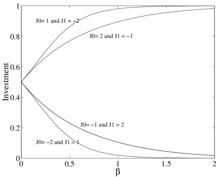
Figure 2: Investment as function of $\beta$ to $q=2$, case $J_{0}/J_{1}<0$

III.2 The three state model: $q=3$

In this case we have the following transfer matrix:

$$M=\left(\begin{array}[]{ccc}e^{-\beta J_{0}}&e^{-\beta D/2}&e^{-\beta D}\\ e^{-\beta D/2}&e^{-\beta(J_{1}+D)}&e^{-3\beta D/2}\\ e^{-\beta D}&e^{-3\beta D/2}&e^{-\beta(J_{2}+2D)}\end{array}\right)$$

The problem of computing eigenvalues is analytically tractable for general values of set $\{J_{0},J_{1},J_{2}\}$ but the expressions obtained are generally very difficult and do not improve our understanding of the problem. However some interesting sub-cases can be considered:

III.2.1 Case 1: $J_{0}=J_{1}=0$ and $J_{2}=J$

In this case by making the change of variables

$$x=e^{-\beta J}\;\;{\mbox{and}}\;\;y=e^{-\beta D/2}$$

we arrive at

$$M=\left(\begin{array}[]{ccc}1&y&y^{2}\\ y&y^{2}&y^{3}\\ y^{2}&y^{3}&xy^{4}\end{array}\right)$$ (13)

One may clearly see that in this matrix the second row is obtained from the first through multiplication by $y$. Hence det$M=0$ and therefore $M$ admits $0$ as an eigenvalue. One may thus compute analytically the other eigenvalues by solving the equation

$$\lambda^{2}-(1+y^{2}+xy^{4})\lambda+(x-1)(y^{4}+y^{6})=0,$$

where the largest eigenvalue is

$$\lambda=\frac{1}{2}\left(1+y^{2}+xy^{4}+\sqrt{\Delta}\right)$$

Here we have

$$\Delta=2y^{2}+5y^{4}+4y^{6}-2xy^{4}-2xy^{6}+x^{2}y^{8}+1\Rightarrow\Delta(D=0)=12-4x+x^{2}$$

and so

$$\begin{array}[]{lllll}l(\beta)&=&-\left.\frac{1}{\beta\lambda}\frac{\partial\lambda}{\partial y}\frac{\partial y}{\partial D}\right|_{D=0}&&\\ &&&&\\ &=&\frac{1}{\left(2+x+\sqrt{12-4x+x^{2}}\right)}\left[1+2x+\frac{12-5x+2x^{2}}{\sqrt{12-4x+x^{2}}}\right]&&\\ &&&&\\ &=&\frac{1}{\left(2+e^{-\beta J}+\sqrt{12-4e^{-\beta J}+e^{-2\beta J}}\right)}\left[1+2e^{-\beta J}+\frac{12-5e^{-\beta J}+2e^{-2\beta J}}{\sqrt{12-4e^{-\beta J}+e^{-2\beta J}}}\right]&&\end{array}$$

One may observe that two cases follow from theorem 3.1: $\beta=0$ and $\beta\to\infty$ when $J<0$. We have $l(0)=1$ and if $J<0$, $l(\beta\rightarrow\infty)=2$. But with the expression for $l$ we can also obtain results beyond the range of the theorem, for example, when $J>0$. In this case $l(\beta\rightarrow\infty)=\frac{1}{2+\sqrt{12}}\left[1+\sqrt{12}\right]$ $=\allowbreak 0.816\,97\cdots$ .

III.2.2 Case 2: $J_{0}=J_{2}=0$ and $J_{1}=J$

In this case we have

$$M=\left(\begin{array}[]{ccc}1&y&y^{2}\\ y&xy^{2}&y^{3}\\ y^{2}&y^{3}&y^{4}\end{array}\right)$$

The discussion is analogous to that of section (III.2.1). The largest eingenvalue is given by

$$\lambda=\frac{1}{2}\left[(y^{4}+xy^{2}+1)+\sqrt{\Delta}\right],$$

with

$$\Delta=4y^{2}+2y^{4}+4y^{6}+y^{8}-2xy^{2}-2xy^{6}+x^{2}y^{4}+1\;.$$

A straighforward calculation gives

$$l(\beta)=1$$

Thus the investment is independent of the parameter $J_{1}$ when $J_{0}=J_{2}=0.$

III.2.3 Case 3: $J_{0}=J$ and $J_{1}=J_{2}=0$

Now $M$ takes the form

$$M=\left(\begin{array}[]{ccc}x&y&y^{2}\\ y&y^{2}&y^{3}\\ y^{2}&y^{3}&y^{4}\end{array}\right)$$

As before we have

$$\lambda=\frac{1}{2}\left[x+y^{2}+y^{4}+\sqrt{\Delta}\right]$$

with

$$\Delta=x^{2}+4y^{2}+5y^{4}+2y^{6}+y^{8}-2xy^{2}-2xy^{4}=x^{2}+12-2x-2x=12+x^{2}-4x$$

For $l(\beta)$ we have the following expression

$$l(\beta)=\frac{1}{\left[e^{-\beta J}+2+\sqrt{12-4e^{-\beta J}+e^{-2\beta J}}\right]}\left(3+\frac{\left(12-3e^{-\beta J}\right)}{\sqrt{12-4e^{-\beta J}+e^{-2\beta J}}}\right)$$

The case $J>0$ is not covered by theorem 3.1. From the expression above we obtain

$$l(\beta\rightarrow\infty)=\frac{3+\sqrt{12}}{2+\sqrt{12}}$$

The only cases where one has analytical solutions are for $q<4$. For other values of $q$ one has to employ numerical methods in order to gain some information, as we discuss in the next section.

IV Numerical analysis

For those cases which are not analytically treatable we can employ an algorithm that combines a routine of numerical derivation with eigenvalues computing. To see how the method work, we first consider the following matrix, written as a function of $\xi$:

$$M(\xi)=\left(\begin{array}[]{ccccc}e^{-\beta\ J_{0}}&e^{-\beta\ \xi/2}&e^{-\beta\xi}&\cdots&e^{-\beta\xi(q-1)/2)}\\ e^{-\beta\xi/2}&e^{-\beta\ (J_{1}+\xi)}&e^{-3\beta\xi/2}&\cdots&e^{-\beta\xi q/2}\\ e^{-\beta\xi}&e^{-3\beta\xi/2)}&e^{-\beta\ (J_{2}+2\xi)}&\cdots&e^{-\beta\xi(q+1)/2}\\ \vdots&\vdots&\vdots&\ddots&\vdots\\ e^{-\beta\xi(q-1)/2}&e^{-\beta\xi q/2}&e^{-\beta\xi(q+1)/2}&\cdots&e^{-\beta\ (J_{q-1}+(q-1)\xi)}\end{array}\right)$$

Let $\lambda_{\xi}$ be the largest eigenvalue corresponding to matrix $M(\xi)$ and $\lambda_{-\xi}$ the one from $M(-\xi)$. If $\xi<<1$ one has:

$$\left.\frac{\partial\lambda}{\partial\xi}\right|_{D=0}=\frac{\lambda_{\xi}-\lambda_{-\xi}}{2\xi}+\sum\limits_{k=1}^{\infty}\frac{\xi^{(2k+1)}\lambda^{(2k+1)}(0)}{2(2k+1)!}$$

since

$$\begin{array}[]{ccc}\lambda_{{}_{\xi}}&=&\lambda_{0}+\lambda_{0}^{\prime}\xi+\frac{\xi^{2}}{2}\lambda_{0}^{\prime\prime}+\frac{\xi^{3}}{3!}\lambda_{0}^{\prime\prime\prime}+...\\ &&\\ \lambda_{{}_{-\xi}}&=&\lambda_{0}-\lambda_{0}^{\prime}\xi+\frac{\xi^{2}}{2}\lambda_{0}^{\prime\prime}-\frac{\xi^{3}}{3!}\lambda_{0}^{\prime\prime\prime}+...\end{array}$$ (14)

A numerical estimate to order ($\ O(\xi^{2})\$) is

$$\Delta^{(1)}\lambda(\xi)=\frac{\lambda_{\xi}-\lambda_{-\xi}}{2\xi}.$$

A more refined numerical estimate can be obtained using not only two but four points $\lambda_{\xi}$, $\lambda_{-\xi},$ $\lambda_{2\xi}$ and $\lambda_{-2\xi}$.

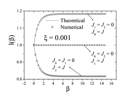
Figure 3: Investment as function of $\beta$ to $q=3$. A comparison of the numerical result with analitical results.

Theorem 3

Consider a function $\lambda\in C^{\infty}(\mathbb{R})$. A numerical approximation to order $O(\xi^{4})$ of $\lambda^{\prime}(D)$ is given by

$$\Delta^{(2)}\lambda(\xi)=-\frac{1}{3}\Delta^{(1)}\lambda(2\xi)+\frac{4}{3}\Delta^{(1)}(\xi)$$

Proof. Considering a Taylor expansion

$$\lambda_{2\xi}=\lambda_{0}+2\xi\lambda_{0}^{\prime}+4\xi^{2}\frac{\lambda_{0}^{\prime\prime}}{2!}+8\xi^{3}\frac{\lambda_{0}^{(3)}}{3!}+16\xi^{4}\frac{\lambda_{0}^{(4)}}{4!}+....$$ (15)

and

$$\lambda_{2\xi}=\lambda_{0}-2\xi\lambda_{0}^{\prime}+4\xi^{2}\frac{\lambda_{0}^{\prime\prime}}{2!}-8\xi^{3}\frac{\lambda_{0}^{(3)}}{3!}+16\xi^{4}\frac{\lambda_{0}^{(4)}}{4!}+....$$ (16)

Combining the equations (14), (15) and (16), we obtain

$$8\lambda_{\xi}-\lambda_{2\xi}+\lambda_{-2\xi}-8\lambda_{-\xi}=12\xi\lambda_{0}^{\prime}-\frac{2}{5}\xi^{5}\lambda_{0}^{(5)}$$

So

$$\lambda_{0}^{\prime}=\left[\frac{\lambda_{2\xi}-\lambda_{-2\xi}}{4\xi}\right]-\frac{4}{3}\left[\frac{\lambda_{\xi}-\lambda_{-\xi}}{2\xi}\right]+O(\xi^{4})$$

which gives us

$$\Delta^{(2)}\lambda(\xi)=-\frac{1}{3}\Delta^{(1)}\lambda(2\xi)+\frac{4}{3}\Delta^{(1)}(\xi)\qquad$$

  

To assess the applicability and performance of the method, we applied it to the integrable $q=3$ case with numerical results using 4–point derivative. In Fig. $3$ we show how the numerical results compare with the analytical ones. By using a higher number of points we observe a significant difference on the results (see Fig. $4$) over selected regions, as compared to a lesser number.

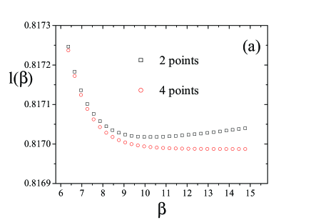
Figure 4: Comparative numerical derivates for $q=3$, using three points and five points. (a) $J_{0}=J_{1}=0$ and $J_{2}=J$; (b) $J_{1}=J_{2}=0$ and $J_{0}=J$; (c) $J_{0}=J_{2}=0$ and $J_{1}=J$.

IV.1 Numerical analysis for $q>3$ considering distinct profiles of agents

In this section we analyze some numerical results for $q>3$. We consider three possible profiles:

1. aggressive or risk-prone agents: in this case the probability of an agent’s investment increase as a function of invested value. We modelled this through

   $$J(\sigma_{i})=-(\sigma_{i}+1)\ <0,$$

   where $\sigma_{i}=0,...,q-1$.

2. conservative agents: the probability of investment decreases as function of invested value. In this situation

   $$J(\sigma_{i})=-(q-\sigma_{i})\ <0,$$

   where $\sigma_{i}=0,...,q-1$.

3. random agents: the probability of the investment is randomly chosen for each agent, such that

   $$J(\sigma_{i})=\left\lfloor\mathop{\mathrm{r}and}[0,1]\cdot q\right\rfloor$$

   where$\ \mathop{\mathrm{r}and}[0,1]$ is a random number uniformly generated in the interval $[0,1]$.

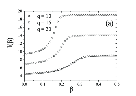
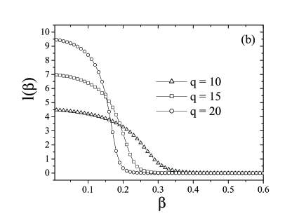
Figure 5: Numerical results for the behavior of investiment as function of $\beta$ for $q=10$, $q=15$ and $q=20$ for two diferent profiles: (a) agressive and (b) conservative.

We generated plots with $q=10,15,20$ for three different profiles. In Fig. 5, we show the risk–prone (a) and conservative (b) profiles. From (a) we conclude that all agents are inclined to invest the maximum quantity for $\beta\rightarrow\infty$ since greater quantities are privileged by the probability distribution. Differently, for (b) as $\beta\rightarrow\infty\$, the investment of each agent goes to $0$. We then may conclude that conservative agents lead to the situation of complete stagnation as $\beta\rightarrow\infty\$, independent of the number possibilities in the investment $q$. On the other hand, risk prone agents lead the market to invest the maximum at this limit.

An alternative profile seems to be more appropriate: The random profile (3) was also explored in an experiment using $12$ seeds (12 different random choices of the string $J(\sigma_{i})$, $i=1...N$) and $q=15$ as depicted in Fig. $6$ ). This figure represents the average over the 12 seeds. The behavior of seeds are not similar in the sense that they may yield different values of investment at $\beta\rightarrow\infty$.

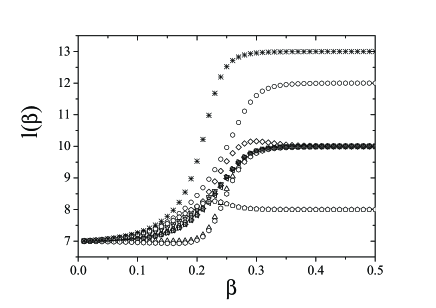
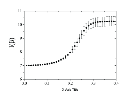
Figure 6: (a) Plot for 12 different seeds for $q=15$; (b) mean value over the seeds.

V Summary and conclusions

We have studied the investment behavior of a group of agents as a function of a parameter that mimics the mean profit obtained by agents. Our results illustrated different situations based on possible investors’ profiles. In a model where $q$ represents the number of possible investment amounts, we obtained analytical results for $q=2$ and $3$. For larger values of $q$ we performed a series of numerical simulations by combining exact diagonalization algorithms with numerical derivatives.

Our results indicate that the behavior of each investor is key to determining the dynamics of the market. As recent results in the context of agents’ simulation show SAAS2004 , pure mathematical models can capture some of the intrincacies of real markets when they, as pointed out in D1999 , try to include real people’s idiosyncrasies (beliefs, sentiments, etc.) that are known to play a significant role (not to mention other important influences as seasonable changes in production, political turmoil, and the like). Even though our model is still mathematical, in the sense that it is based on a well known model of statistical mechanics and we identify behavior in terms of known physical quantities, we believe that our ideas might help indicate a way towards a more realistic market modelling.

Aknowledgments

The authors thank A. C. Bazzan for enlightening discussions

References

- (1) R. da Silva, A. C. Bazzan, A. Baraviera, S. R. Dahmen, “Emerging Collective Behavior in a Simple Artificial Financial Market”, to be published in: Proc. IV Int. Joint Conference on Autonomous Agents and Multi-Agent Systems (AAMAS), Utrecht (2005)
- (2) A. Dragulescu, V. M. Yakovenko, Eur. Phys. J. B17, 723-729 (2000)
- (3) W. Brock, Stud. Econ. 8, 3-55 (1993)
- (4) L. Blume, Games Econ. Behav. 5, 387-424 (1993)
- (5) S. N. Durlauf, Proc. Natl. Acad. Sci. USA 96, 10582-10584 (1999)
- (6) F. W. Wu, Rev. Mod. Phys. 54, 235 (1982)
- (7) R. Mantegna, H. E. Stanley, “An Introduction to Econophysics”, Cambridge Univ. Press, Cambridge, (2000)
- (8) K. Huang, “Statistical Mechanics”, John Wiley, New York, (1987)