Current address.]

Evidence for Macroscopic Quantum Tunneling of Phase Slips in Long One-Dimensional Superconducting Al Wires

Abstract

Quantum phase slips have received much attention due to their relevance to superfluids in reduced dimensions and to models of cosmic string production in the Early Universe. Their establishment in one-dimensional superconductors has remained controversial. Here we study the nonlinear voltage-current characteristics and linear resistance in long superconducting Al wires with lateral dimensions $\sim$ 5 nm.We find that, in a magnetic field and at temperatures well below the superconducting transition, the observed behaviors can be described by the non-classical, macroscopic quantum tunneling of phase slips, and are inconsistent with the thermal-activation of phase slips.

What is the resistance of a superconductor below its superconducting transition temperature? For a three-dimensional superconductor, the answer is the obvious one – zero. But in one-dimension (1D), by which we mean very thin very long wires, quantum fluctuations destroy the zero resistance state. Phase slips – small superconducting regions that become normal, allowing the phase of the order parameter to rapidly change by $2\pi$ – give rise to residual resistance and can even quench superconductivity completely. The tiny cross-section of 1D nanowires reduces the free energy barrier arising from a loss of condensation energy for the creation of phase slips. Thermal activation of phase slips (TAPS) across this barrier is responsible for the residual resistance just below $T_{c}$ (LAMH picture) Langer and Ambegaokar (1967). On the other hand, macroscopic quantum tunneling of phase slips (QTPS) as the source of residual resistance at low temperatures has remained controversial despite intense experimental effort Giordano (1988); Duan (1995); Bezryadin et al. (2000); Lau et al. (2001); Tian et al. (2005); Savolainen et al. (2004); Rogachev et al. (2005). The observation of macroscopic quantum tunneling is of significance not only for 1D superconductivity, but also for understanding the decoherence of quantum systems due to interaction with their environment. Here we clearly establish the presence of QTPS in superconducting (SC) Al nanowires, showing the dramatic effect they have on the voltage-current (V-I) characteristics of the wire.

Phase slips in 1D SC nanowires have traditionally been studied by measuring the linear resistance as a function of the temperature through the normal-superconducting (N-S) transition. Any resistance in excess to that predicted by thermal activation is attributed to macroscopic tunneling of phase slips Giordano (1988); Duan (1995); Bezryadin et al. (2000); Lau et al. (2001); Tian et al. (2005); Savolainen et al. (2004). However, this attribution can be flawed because of weak links in the wire resulting from inhomogeneities Duan (1995); Savolainen et al. (2004). Moreover, the fitting of the excess residual resistance to quantum-phase-slip expressions Giordano (1988); Lau et al. (2001); Savolainen et al. (2004); Tian et al. (2005) often necessitated an ad hoc reduction in the free-energy barrier. Recently Rogachev et al. Rogachev et al. (2005) examined the nonlinear V-I dependence of $Mo_{0.79}Ge_{0.21}$ SC nanowires: they found that the deduced residual resistance, spanning 11 orders in magnitude, followed the prediction of classical TAPS alone, thus contradicting previous claims of QTPS behavior based on residual linear resistance by the same group Bezryadin et al. (2000); Lau et al. (2001).

In this Letter, we examine the nonlinear V-I characteristics and linear resistance of long aluminum nanowires, the narrowest one with dimension 5.2 nm x 6.1 nm x 100 $\mu$m (21 x 24 x 400,000 atoms). Our wires are much longer than those of similar cross section reported in the literature ($\sim 0.5\mu$m long)Bezryadin et al. (2000); Lau et al. (2001); Rogachev et al. (2005) and the ratio of the low temperature SC coherence length to the width (or height) is also much larger, thus placing us in a regime distinct from previous works. Specifically, we study the residual resistance deduced from the nonlinear V-I characteristics in the superconducting state below the critical current. Our main finding is that the V-I dependence and residual resistance are inconsistent with the classical LAMH behavior, but instead are well described by quantum expressions, either derived from an extension of the classical model Giordano (1988) or in a recently proposed power-law form Golubev and Zaikin (2001); khl (a, b). The good fits to the different quantum expressions, which closely overlap each other, are corroborated by measured residual linear resistance, achieving full consistency within the quantum scenario using a single set of fitting parameters. Our results demonstrate the importance of non-classical, quantum phase slips in ultranarrow, 1D superconducting aluminum wires.

The nanowires were fabricated by thermally evaporating aluminum onto a narrow, 8 nm-wide, MBE (molecular-beam-epitaxy) grown InP ridge, while at once linking and partially covering the four-terminal Au/Ti measurement pads (Fig. 1(b)). The fabrication is described elsewhereAltomare et al. (2005). Magnetoresistance at 4.2 K (above $T_{c}$) was used to characterize the wires (Table 1). The calculated dirty limit $\xi$ TinkhamBook ($\approx$ 94 nm for s1, $\approx$ 128 nm for s2) far exceeds the lateral dimensions ($\sim 5-9$ nm).

	$L$	$w$	$t$	$R_{N}$	$\rho$	$l_{e}$	$\xi$	$J_{c}$ (0.35 K)
	$\mu$m	nm	nm	$k\Omega$	$\mu\Omega cm$	nm	nm	$10^{5}A/cm^{2}$
s1	10	6.9	9.0	8.3	5.1	7.6	94	12.1
s2	100	5.25	6.09	86	2.8	14.3	128	13.1

Table 1: Parameters for sample s1 and s2, including $L$ (length), $w$ (width), $t$ (thickness), $R_{N}$ (normal state resistance), $\rho$ (resistivity), $l_{e}$ (mean free path), $\xi$ (GL coherence length), and $J_{c}$ (critical current density). $w$, $t$, $\rho$ and $l_{e}$ were deduced based on magnetoresistance measurements Altomare et al. (2005). $\xi$ was calculated using $\xi\!=\!0.85\sqrt{\xi_{0}l_{e}}$ where $\xi_{0}\!=\!1600~{}nm$ is the GL superconducting coherence length in bulk aluminum.

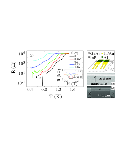
Figure 1: (Color) (a) Linear resistance versus temperature for wire s2 in different magnetic fields; the pad series resistance has been subtractedprl (b). Inset: The pad series resistance increases at magnetic fields beyond the critical field of the pad regions covered by aluminum (T=0.38, 0.80, 0.99, 1.10 K). (b)-(d) Schematic and SEM images of a nominally 8 nm wide Al nanowire (similar to samples s1 and s2): the Al layer does not entirely cover the Au/Ti pads which were measured in series with the superconducting wire.

To investigate the SC behavior, the linear resistance through the N-S transition was measured at a current of 1.6 nA (Fig. 1(a)), while the nonlinear V-I characteristics was measured in both the constant-current (Figs. 2(a)-(b) and 3) and constant-voltage modes below $T_{c}$ prl (a). The linear resistance drops by several orders of magnitude from the normal state resistance ($R_{N}$) through $T_{c}$, but remains finite. In Fig. 1(a) we show the linear resistance versus temperature for wire s2 in different magnetic fields ($H$)prl (b). At a given temperature, the resistance increases with increasing $H$ as superconductivity weakens. In the constant-current mode, finite residual nonlinear voltage is observed in the V-I curves below the critical current jump. Such residual voltage is unobservable in large wires. In the constant-voltage mode, the V-I curves exhibit non-hysteretic voltage steps and S-shaped curves down to $T/T_{c}\approx 0.2$, typical of 1D superconductors Tian et al. (2005); Vodolazov et al. (2003). Evidences for wire homogeneity include: 1) comparable critical current density in wires s1 and s2 2) all V-I traces in the constant-current mode showed a single critical current jump.

To assess the importance of QTPS, we focus on the residual resistance and residual voltage below $T_{c}$ for sample s2; the wider s1 will be used for control as discussed below. The main datasets consist of the nonlinear V-I curves in constant-current mode (Figs. 2(a)-(b) and 3 (black curves)), and the linear resistance versus $T$. This latter resistance is obtained in two ways: (i) from the data in Fig. 1(a) prl (b) (Figs. 2(c)-(d) (black curves)), and (ii) from the fits to the nonlinear V-I curves according to Eqs. (1b) and (3) below ($\boldsymbol{\boldsymbol{\bm{\bigtriangleup}}}$, Figs. 2(e)-(f)). It will be demonstrated through quantitative analysis that this entire set of data is inconsistent with the TAPS scenario, as evidenced by the poor fits to the LAMH expressions (Eqs. (1a) and (1b)) shown in Figs. 2 and 3 (blue curves). Instead the inclusion of the QTPS contributions (Giordano (GIO) model Eqs. (2) and (3)) in the fits is essential in providing a fully consistent description based on a single set of parameters (see red curves in Figs. 2 and 3).

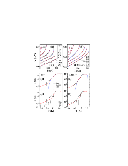
Figure 2: (Color) Nonlinear V-I curves and linear resistance for sample s2 at different magnetic fields ($H$): Black curves–data; red curves–fits to the GIO ($\equiv$GIO + LAMH) expressions for QPS ($\equiv$TAPS + QTPS), and blue curves–fits to the LAMH expressions for TAPS alone. (a)-(b) V-I curves offset for clarity. The fits to QPS are of higher quality compared to TAPS; each fit includes a series resistance term $V_{S}$. These V-I curves can be fitted equally well by a power law form $V=V_{S}+K\cdot(I/I_{k})^{\nu}$ where $12\gtrsim\nu\gtrsim 3.2$ for $0\leq H\leq 1.05$ Tkhl (a, b). (c)-(d) Linear resistance after background subtraction (see Fig. 1(a) and prl (b)). The LAMH fits are poor at low $T$. (e)-(f) The resistance contribution due to phase slips ($R_{QPS}$) extracted in (a)-(b) from fits to the V-I curves using the GIO expressions (discrete points, $\boldsymbol{\boldsymbol{\bm{\bigtriangleup}}}$). $R_{QPS}$ and the linear resistance from (c)-(d) are refitted using the GIO expressions (red) with the same $a_{GIO}(=1.2)$ while disregarding the irrelevant shoulder feature (dashed line).

Thermal activation of phase slips, important at $T\lesssim T_{c}$, is well described by the expressions derived by Langer Ambegaokar, McCumber, Halperin (LAMH)Langer and Ambegaokar (1967); prl (c):

$$R_{LAMH}\!=\!R_{q}\displaystyle{\frac{\Omega}{k_{B}T}}\exp{\left(\displaystyle{-\frac{\Delta F}{k_{B}T}}\right)},$$ (1a)

$$V_{TAPS}\!=\!I_{0}R_{LAMH}\sinh{\left(I/I_{0}\right)},$$ (1b)

where the quantum resistance $R_{q}\!=\!\pi\hbar/2e^{2}$, attempt frequency $\Omega\!=\!(L/\xi)(\Delta F/k_{B}T)^{1/2}(\hbar/\tau_{\scriptscriptstyle GL})$, free energy barrier $\Delta F\!=\!(8\sqrt{2}/3)(H_{th}^{2}/8\pi)A\xi$, and Ginzburg-Landau relaxation time $\tau_{\scriptscriptstyle GL}\!=\!(\pi/8)[\hbar/k_{B}(T-T_{c})]$, $I_{0}\!=\!4ek_{B}T/h$. $L$ is the wire length, $T$ the temperature, $k_{B}$ the Boltzmann constant, $H_{th}$ the thermodynamical critical field, $A$ the wire cross section, and $\xi$ the GL coherence length.

Quantum tunneling of phase slips, which takes place in parallel with thermal activation, is expected to dominate at low $T$. GiordanoGiordano (1988) proposed a quantum form by replacing $kT$ with $(1/a_{GIO})(\hbar/\tau_{GL})$prl (c); GIO :

$$R_{GIO}\!=R_{q}\frac{L}{\xi}\sqrt{a_{GIO}\frac{\Delta F}{\hbar/\tau_{\scriptscriptstyle GL}}}\exp{\left(-a_{GIO}\frac{\Delta F}{\hbar/\tau_{\scriptscriptstyle GL}}\right)}$$ (2)

where $a_{GIO}$ is a numerical constant of order unity and, in analogy with the thermal case, we propose thatprl (c); GIO :

$$V_{QTPS}\!=\!I_{GIO}R_{GIO}\sinh{\left(I/I_{GIO}\right)}$$ (3)

where $I_{GIO}\!=\!2e/(\pi\tau_{\scriptscriptstyle GL}a_{GIO})$. In this quantum case, a resistance similar to the Giordano expression (and numerically equivalent) has been recently derived, on a microscopic basis, by Golubev and Zaikin Golubev and Zaikin (2001) and by Khlebnikov and Pryadko khl (a). In the nonlinear regime, both theories predict a crossover from an exponential dependence to a power-law behavior ($V\propto I^{\nu}$) at low $T$.

To begin the analysis, we first extract the parameters, $T_{c}$ and $\xi$ at each magnetic field and a single $a_{GIO}$, by fitting to the linear $R$ versus $T$ traces in Figs. 2(c)-(d); $T_{c}$ and $a_{GIO}$ are input parameters in the analysis of the V-I curves. Below $T_{c}$, a wire is modeled as a normal and a superconducting wire in parallel, the latter with a resistance produced by the relevant phase slips mechanismLau et al. (2001). To account for the shoulder feature at a resistance $\approx 1/20$ of $R_{N}$, we assume our wire to be composed of segments of two slightly different cross sectional areas, with a fixed ratio of 90% ($\Delta F\!\propto\!A$). The thinner segments corresponding to the smaller cross sectional area have a larger $T_{c}$Savolainen et al. (2004). These segments, with critical temperature (resistance) $T_{c1}$ ($R_{1}$), are responsible for $\gtrsim{}$95% of $R_{N}$. At zero field, the fitting parameters are $T_{c1}(H\!=\!0)$, $T_{c2}(H\!=\!0)$, $\xi(H\!=\!0)$, $R_{1}$, and $a_{GIO}$, while at $H\geq 0.465$ T, only $T_{c1}(H)$, $T_{c2}(H)$, $\xi(H)$ are varied. Fitting using two $\xi$s produced unphysical $\xi$ dependence on $H$ and was discarded. The fits to the GIO (red) and LAMH (blue) theory are presented in Figs. 2(c)-(d). At $H=0$ T both fits reproduced the data over several decades in resistance and are nearly equivalent above $\approx$5 $\Omega$. At higher field the GIO theory better models the data, particularly at low $T$reb_3_1 . The fitting parameters $T_{c1}$ and $\xi$ ($\boldsymbol{\boldsymbol{\bm{\circ}}}$) are presented in Fig. 4 (a)-(b). Their $H$ dependence can be fitted to simple theoretical expressions as shown. The single value of $a_{GIO}\!=\!1.2$ we obtain, of order unity as expected, will be used throughout all the subsequent analysis.

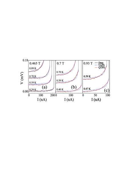
Figure 3: (Color) The nonlinear V-I curves, at $T/T_{c}\lesssim 0.5$ are refitted with $V=V_{QTPS}+V_{S}$ and $V=V_{TAPS}+V_{S}$ (see text).(a)-(c) The data (black), QTPS (red) and TAPS (blue) fits and are shown after subtracting the linear background. Dotted (dashed) line in 3(a) is the fit to the TAPS expression with a 50% reduction (increase) in temperature, respectively.

Despite the success in fitting to the linear resistance, it is not possible to completely rule out weak links as the source of residual resistance. To clearly demonstrate the importance of quantum phase slips, it is necessary to analyze the nonlinear V-I dependence. Generalizing the nonlinear analysis of Rogachev et al.Rogachev et al. (2005) by including QTPS while also accounting for series resistances, the total voltage drop across the superconducting nanowire is $V\!=\!V_{TAPS}+V_{QTPS}+V_{S}$, where  $V_{TAPS}$ and $V_{QTPS}$ are given in Eqs. (1b) and (3), respectivelyprl (c), and $V_{S}\!=\!R_{S}I$. $R_{S}$ is a series resistance which includes the contribution of the pads and other ohmic-like contributions such as proximity effect of the normal pads on the SC wireBoogaard et al. (2004). The fitting parameters are $R_{TAPS}$, $R_{QTPS}$ and $R_{S}$prl (c), while $a_{GIO}(=\!1.2)$ and $T_{c}(H)$, which enters through $\tau_{\scriptscriptstyle GL}$, are taken from the previous fits (Fig. 4(a)). At all temperatures and fields, the fitting curves reproduce the data extremely well, as shown in red in Figs. 2(a)-(b) and 3prl (b). At higher $T$ ($T/T_{c}\gtrsim 0.7$) the contribution from QTPS is negligible compared to TAPS. At low $T$ ($T/T_{c}$ $\lesssim 0.5$) TAPS is expected to be exponentially suppressed (Eq. (1a)) and QTPS should dominate; this expectation is confirmed by the fits which yielded a negligible $R_{TAPS}$ compared to $R_{QTPS}$prl (b).

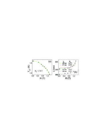
Figure 4: (Color) GIO($\equiv$GIO+LAMH) fitting parameters to the linear resistance curves, including those shown in Fig. 2(c)-(d), plotted versus $H$. (a) $T_{c1}$ ($\boldsymbol{\boldsymbol{\bm{\diamond}}}$) and $T_{c2}$ (not shown) fit well to the pair breaking perturbation theoryTinkhamBook (green). (b) $\xi$ ($\boldsymbol{\boldsymbol{\bm{\circ}}}$) is fitted to both $\xi\!=\!\xi_{c}/\sqrt[4]{1-(H/H_{c})^{2}}$ (magenta) ($\Delta\!\propto\!\sqrt{1-(H/H_{c})^{2}}$ and $\xi\!\propto\!1/\sqrt{\Delta}$TinkhamBook ), and to an ad hoc expression $\xi\!=\!\xi_{c}/\sqrt{1-(H/H_{c})^{2}}$ (green); $\xi_{c}\!\equiv\!\xi(H\!=\!0)$ and  $H_{c}$ is the critical field. $\xi$ is better described by the ad hoc expression. $\xi$ ($\boldsymbol{\boldsymbol{\bm{\bigtriangleup}}}$) derived from the fits to $R_{QPS}$, including those in Fig. 2. (e)-(f), is fitted to theory as before (dashed lines) yielding $\xi_{c}\approx 135~{}nm$, within 5% of the value in Table 1.

To further substantiate the importance of QTPS at low $T$ while at the same time rule out TAPS as a significant cause of phase slips, we directly compare fits of the nonlinear V-I curves using $V=V_{QTPS}+V_{S}$ and $V=V_{TAPS}+V_{S}$. The fitting parameters for QTPS are $R_{QTPS}$, $R_{s}$, and for TAPS they are $R_{TAPS}$, $R_{S}$. The curves are presented in Figs. 3(a)-(c) after subtracting the linear background for several $H>0$ T. Although the two expressions have the same number of parameters, the QTPS fits (red) are of good quality while the TAPS fits (blue) are evidently much poorer. Varying $T$ by $\pm 50\%$ in the TAPS fits still failed to reproduce the data, as shown in Fig. 3(a) for $T=0.59$ K and $H=0.465$ T. Comparing the $\chi$-squares of the fits that include QTPS versus TAPS alone using the statistical F-test yielded strong support for the importance of quantum phase slips with a confidence level $>$99.99%prl (d).

The $R_{QPS}=R_{QTPS}+R_{TAPS}$ extracted from the nonlinear V-I fits enables to exclude contributions to residual resistance that are irrelevant to phase slips, providing a means to check full consistency. In Figs. 2(e)-(f) we plot $R_{QPS}$ ($\boldsymbol{\boldsymbol{\bm{\bigtriangleup}}}$ symbols) for $T\lesssim T_{c}$ and replot the linear resistance through the N-S transition for comparison; we then refit the linear resistance expressions (GIO+LAMH, Eqs. (1a) + (2)) to these data, keeping $a_{GIO}=1.2$ unaltered while varying $T_{c}$ and $\xi$. The discrete $R_{QPS}$ data points versus $T$ no longer exhibit a shoulder feature, and only one $T_{c}$ was needed. Satisfactory agreement is achieved as depicted in Figs. 2(e)-(f) (red). Similar agreement comparable to the $H=0.465$ T trace is obtained at higher $H=0.7$ T, 0.93 T, etc. $T_{c}$ was essentially unchanged compared to $T_{c1}$ in Fig. 4(a) but $\xi$ (Fig. 4(b), $\boldsymbol{\boldsymbol{\bm{\bigtriangleup}}}$) was reduced at higher $H$, compared to the data obtained previously (Fig. 4(b), $\boldsymbol{\boldsymbol{\bm{\circ}}}$). Fitting to the new values yielded $\xi_{c}\equiv\xi(H\!=\!0)\approx 135~{}nm$, within 5% of the calculated value in Table 1. As a final consistency check, analysis of the wider superconducting sample s1Altomare et al. (2005) did not produce any sign of QTPS for $H\lessapprox 0.9$ T. This is sensible because of the larger free-energy barrier.

The consistency achieved in our analysis of the nonlinear V-I curves and residual resistance, supported by the quantitative statistical F-test, demonstrates the importance of quantum phase slips. This helps rule out other scenarios, e.g. TAPS alone or weak links. Furthermore, our results establish that the transport properties of 1D superconducting nanowires at temperatures much below $T_{c}$ are determined primarily by the macroscopic quantum tunneling of phase slips. Our findings pave the way to the study of newly predicted quantum phase transitions in metallic nanowiresSachdev et al. (2004).

F.A. thanks M.E. Rizza for her support. Work supported by NSF DMR-0135931 and DMR-0401648.

References

- Langer and Ambegaokar (1967) J. S. Langer and V. Ambegaokar, Physical Review 164, 498 (1967); D. E. McCumber and B. I. Halperin, Phys. Rev. B 1, 1054 (1970).
- Giordano (1988) N. Giordano, Phys. Rev. Lett. 61, 2137 (1988).
- Duan (1995) J. M. Duan, Phys. Rev. Lett. 74, 5128 (1995).
- Bezryadin et al. (2000) A. Bezryadin et al., Nature 404, 971 (2000).
- Lau et al. (2001) C. N. Lau et al., Phys. Rev. Lett. 87, 217003 (2001).
- Tian et al. (2005) M. L. Tian et al., Phys. Rev. B 71, 104521 (2005).
- Savolainen et al. (2004) M. Savolainen et al., Appl. Phy. A 79, 1769 (2004); M. Zgirski et al., Nano Letters 5, 1029 (2005).
- Rogachev et al. (2005) A. Rogachev et al., Phys. Rev. Lett. 94, 017004 (2005).
- Golubev and Zaikin (2001) D. S. Golubev and A. D. Zaikin, Phys. Rev. B 64, 014504 (2001).
- khl (a) S. Khlebnikov and L. P. Pryadko, Phys. Rev. Lett. 95, 107007 (2005).
- khl (b) EPAPS Document No. (Section 1) summarizes the magnetic field behavior of the exponent.
- Altomare et al. (2005) F. Altomare et al., Appl. Phys. Lett. 86, 172501 (2005).
- (13) Tinkham M., Introduction to Superconductivity, (1996).
- prl (a) Linear resistance measurements were performed with a lockin-amplifier at 23 Hz. Room temperature filters and low temperature RC filters, formed naturally from the sample lead resistances (2-20 ) and capacitances to ground (0.5 nF), helped reduce noise to the nanowires.
- prl (b) See EPAPS Document No. (Section 2) .
- Vodolazov et al. (2003) D. Y. Vodolazov et al., Phys. Rev. Lett. 91, 157001 (2003).
- prl (c) To distinguish the fitting parameters from the theoretical values, we refer to () as the TAPS (QTPS) resistance extracted from fits to the V-I, and to () as the calculated values for TAPS (QTPS).
- (18) In the following, when referring to the GIO theory, we will implicitly include the LAMH contribution as well.
- (19) At sufficiently high -field, the rapid increase in and decrease in reduces the free energy barrier ([6] (Fig. 4(a)-(b)). For a given intermediate temperature the contribution from TAPS can actually become larger.
- Boogaard et al. (2004) G. R. Boogaard et al., Phys. Rev. B 69, 220503(R) (2004).
- prl (b) The establishment of the nanowire electron temperature is in Section 4 of the EPAPS Document No.
- prl (b) For the data central to QTPS shown in Figs. 2(f) and Fig. 3, there were a total of 21 fitting parameters for 1106 data points in the 10 traces, or 53 points per parameter.
- prl (d) See EPAPS Document No. (Section 3) for F-test details.
- Sachdev et al. (2004) S. Sachdev et al., Phys. Rev. Lett. 92, 237003 (2004).