A Decomposition Approach to Multi-Vehicle Cooperative Control

Abstract

We present methods that generate cooperative strategies for multi-vehicle control problems using a decomposition approach. By introducing a set of tasks to be completed by the team of vehicles and a task execution method for each vehicle, we decomposed the problem into a combinatorial component and a continuous component. The continuous component of the problem is captured by task execution, and the combinatorial component is captured by task assignment. In this paper, we present a solver for task assignment that generates near-optimal assignments quickly and can be used in real-time applications. To motivate our methods, we apply them to an adversarial game between two teams of vehicles. One team is governed by simple rules and the other by our algorithms. In our study of this game we found phase transitions, showing that the task assignment problem is most difficult to solve when the capabilities of the adversaries are comparable. Finally, we implement our algorithms in a multi-level architecture with a variable replanning rate at each level to provide feedback on a dynamically changing and uncertain environment.

1 Introduction

Using a team of vehicles to accomplish an objective can be effective for problems involving a set of tasks distributed in space and time. Examples of such problems include multi-target intercept [1], terrain mapping [24], reconnaissance [28], and surveillance [36]. To achieve effective solutions, in general, a vehicle team needs to follow a cooperative policy. The generation of such a policy has been the subject of a rich literature in cooperative control. A sample of the noteworthy work in this field includes a language for modeling and programming cooperative control systems [18], receding horizon control for multi-vehicle systems [9], non-communicative multi-robot coordination [21], hierarchical methods for target assignment and intercept [1], cooperative estimation for reconnaissance problems [28], mixed integer linear programming methods for cooperative control [33, 13], the compilation on multi-robots in dynamics environments [22], and the compilation on cooperative control and optimization [26].

When multi-vehicle teams operate in dynamically changing and uncertain environments, which is often the case, a model predictive approach [23] can be used to provide feedback. This approach involves frequently recomputing the team control policy in real-time. However, because these systems are often hybrid dynamical systems, computing a cooperative policy is often computationally hard. The challenge addressed in this paper is to (1) develop a method to generate near-optimal cooperative policies quickly and (2) to effectively implement the method.

In our previous work on cooperative control [13, 11] we developed mixed integer linear programming methods because of their expressiveness and ease of modeling many types of problems. The drawback is that real-time planning is infeasible because of the computational complexity of the approach. This motivated us to develop a trajectory primitive decomposition approach to the problem. This approach finds near-optimal solutions quickly, allowing real-time implementation, and can be tuned to balance the tradeoff between optimality and computational effort for the particular problem at hand. The drawback, compared to our previous work, is that it is limited to cooperative control problems in which vehicle tasks can be clearly defined and efficient primitives exist.

In this paper, we present our trajectory primitive decomposition approach. We analyze the average case behavior of the approach by solving instances of a cooperative control problem derived from Cornell’s RoboFlag environment. And finally, we implement the approach in a hierarchical architecture with variable replanning rates at each level and test the implementation in a dynamically changing and uncertain RoboFlag environment.

The trajectory primitive decomposition involves the introduction of a set of tasks to be executed by the vehicles, allowing the problem to be separated into a low-level component, called task execution, and a high-level component, called task assignment. The task execution component is formulated as an optimal control problem, which explicitly involves the vehicle dynamics. Given a vehicle and a task, the goal is to find the control inputs necessary to execute the given task in an optimal way. The task assignment component is an NP-hard [14] combinatorial optimization problem. The goal is to assign a sequence of tasks to each vehicle so that the team objective is optimized. Task assignment does not explicitly involve the vehicle dynamics because the task execution component is utilized as a trajectory primitive.

We have developed a branch and bound algorithm to solve the task assignment problem. One of the benefits of this algorithm is that it can be stopped at any time in the solution process and the output is the best feasible assignment found in that time. This is advantageous for real-time applications where control strategies must be generated within a time window. In this case, the best solution found in the time window is used. Another advantage is that the algorithm is complete; given enough time, it will find the optimal solution.

To analyze the average case performance of the branch and bound solver, we generate and solve many instances of the problem. We look at computational complexity, convergence to the optimal assignment, and performance variations with parameter changes. We found that the solver converges to the optimal assignment quickly. However, the solver takes much more time to prove the assignment is optimal. Therefore, if the solver is terminated early, the best feasible assignment found in that time is likely to be a good one. We also found several phase transitions in the task assignment problem, similar to those found in the pioneering work [20, 34, 25]. At the phase transition point, the task assignment problem is much harder to solve. For cooperative control problems involving adversaries, the transition point occurs when the capabilities of the two teams are comparable. This behavior is similar to the complexity of balanced games like chess [16].

Finally, we implement the methods in a multi-level architecture with replanning occurring at each level, at different rates (multi-level model predictive control). The motivation is to provide feedback to help handle dynamically changing environments.

The paper is organized as follows: In Section 2, we state the multi-vehicle cooperative control problem and introduce the decomposition. In Section 3, we introduce the example problem used to motivate our approach. In Section 4, we describe our solver for the task assignment problem, and in Section 5, we analyze its average case behavior. Finally, in Section 6, we apply our solver in a dynamically changing and uncertain environment using a multi-level model predictive control architecture for feedback. A web page that accompanies this paper can be found at [10].

2 Multi-vehicle task assignment

The general multi-vehicle cooperative control problem consists of a heterogeneous set of vehicles (the team), an operating environment, operating constraints, and an objective function. The goal is to generate a team strategy that minimizes the objective function. The strategy in its lowest level form is the control inputs to each vehicle of the team.

In [11, 13], we show how to solve this problem using hybrid systems tools. This approach is successful in determining optimal strategies for complex multi-vehicle problems, but becomes computationally intensive for large problems. Motivated to find faster techniques, we have developed a decomposition approach described in this paper.

The key to the decomposition is to introduce a relevant set of tasks for the problem being considered. Using these tasks, the problem can be decomposed into a task completion component and a task assignment component. The task completion component is a low level problem, which involves a vehicle and a task to be completed. The task assignment component is a high level problem, which involves the assignment of a sequence of tasks to be completed by each vehicle in the team.

Task Completion: Given a vehicle, an operating environment with constraints, a task to be completed, and an objective function, find the control inputs to the vehicle such that the constraints are satisfied, the task is completed, and the objective is minimized.

Task Assignment: Given a set of vehicles, a task completion algorithm for each vehicle, a set of tasks to be completed, and an objective function, assign a sequence of tasks to each vehicle such that the objective function is minimized.

In the task assignment problem, instead of varying the control inputs to the vehicles to find an optimal strategy, we vary the sequence of tasks assigned to each vehicle. This problem is a combinatorial optimization problem and does not explicitly involve the dynamics of the vehicles. However, in order to calculate the objective function for any particular assignment, we must use the task completion algorithm. Task completion acts as a primitive in solving the task assignment problem, as shown by the framework in Figure 1. Using the low level component (task completion), the high level component (task assignment) need not explicitly consider the detailed dynamics of the vehicles required to perform a task.

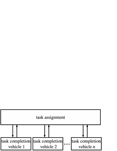
Figure 1: The framework for the task assignment problem using task completion primitives.

3 RoboFlag Drill

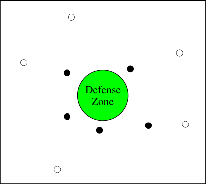
Figure 2: The RoboFlag Drill used to motivate the methods presented is this paper. The drill takes place on a playing field with a Defense Zone at its center. The objective is to design a cooperative control strategy for the team of defending vehicles (black) that minimizes the number of attacking vehicles (white) that enter the Defense Zone.

To motivate and make concrete our decomposition approach, we illustrate the approach on an example problem derived from Cornell’s multi-vehicle system called RoboFlag. For an introduction to RoboFlag, see the papers from the invited session on RoboFlag in the Proceedings of the 2003 American Control Conference [3, 7, 8]. In [19], protocols for the RoboFlag Drill are analyzed using a computation and control language.

The RoboFlag Drill involves two teams of vehicles, the defenders and the attackers, on a playing field with a circular region of radius $R_{dz}$ at its center called the Defense Zone (Figure 2). The attackers’ objective is to fill the Defense Zone with as many attackers as possible. They have a fixed strategy in which each moves toward the Defense Zone at constant velocity. An attacker stops if it is intercepted by a defender or if it enters the Defense Zone. The defenders’ objective is to deny as many attackers as possible from entering the Defense Zone without entering the zone themselves. A defender denies an attacker from the Defense Zone by intercepting the attacker before it reaches the Defense Zone.

The wheeled vehicles of Cornell’s RoboCup Team [37, 6] are the defenders in the RoboFlag Drill problem we consider in this paper. Each vehicle is equipped with a three-motor omni-directional drive that allows it to move along any direction irrespective of its orientation. This allows for superior maneuverability compared to traditional nonholonomic (car-like) vehicles. A local control system on the vehicle, presented in [27] and Appendix A, alters the dynamics so that at a higher level of the hierarchy, the vehicle dynamics are governed by

$$\ddot{x}(t)+\dot{x}(t)=u_{x}(t)$$

$$\ddot{y}(t)+\dot{y}(t)=u_{y}(t)$$

$$u_{x}(t)^{2}+u_{y}(t)^{2}\leq 1.$$ (1)

The state vector is $\mathbf{x}=(x,y,\dot{x},\dot{y})$, and the control input vector is $\mathbf{u}=(u_{x},u_{y})$. These equations are less complex than the nonlinear governing equations of the vehicles. They allow for the generation of feasible near-optimal trajectories with little computational effort and have been used successfully in the RoboCup competition.

Each attacker has two discrete modes: active and inactive. When active, the attacker moves toward the Defense Zone at constant velocity along a straight line path. The attacker, which is initially active, transitions to inactive mode if the defender intercepts it or if it enters the Defense Zone. Once inactive, the attacker does not move and remains inactive for the remainder of play. These dynamics are captured by the discrete time equations

$$p[k+1]=p[k]+v_{p}Ta[k]$$

$$q[k+1]=q[k]+v_{q}Ta[k]$$ (2)

and the state machine (see Figure 3)

$$a[k+1]=\left\{\begin{array}[]{ll}1&\mbox{if ($a[k]=1$)}\\ &\mbox{and (not in Defense Zone)}\\ &\mbox{and (not intercepted) }\\ 0&\mbox{if ($a[k]=0$)}\\ &\mbox{or (in Defense Zone)}\\ &\mbox{or (intercepted)}\end{array}\right.$$ (9)

Figure 3: The two state (active and inactive) attacker state machine. The attacker starts in the active state. It transitions to the inactive state, and remains in this state, if it enters the Defense Zone or if it is intercepted by a defender.

for all $k$ in the set $\{1,\ldots,N_{a}\}$. The initial conditions are

$$\mbox{$p[0]=p_{s}$, $q[0]=q_{s}$, and $a[0]=1$}.$$ (10)

In these equations, $N_{a}$ is the number of samples, $T$ is the sample time, $(p[k],q[k])$ is the attacker’s position at time $t_{a}[k]=kT$, $(v_{p},v_{q})$ is its constant velocity vector, and $a[k]\in\{0,1\}$ is a discrete state indicating the attacker’s mode. The attacker is active when $a[k]=1$ and inactive when $a[k]=0$. Given $(p[k],q[k])$ and $a[k]$, we can calculate the attacker’s position at any time $t$, denoted $\mathbf{p}(t)=(p(t),q(t))$, using the equations

$$p(t) {}={} p[k]+v_{p}a[k](t-t_{a}[k])$$

$$q(t) {}={} q[k]+v_{q}a[k](t-t_{a}[k]),$$ (11)

where $k=\lfloor t/T\rfloor$.

Because the goal of the RoboFlag Drill is to keep attackers out of the Defense Zone, attacker intercept is an obvious task for this problem. Therefore, the task completion problem for the RoboFlag Drill is an intercept problem.

RoboFlag Drill Attacker Intercept (RDAI): Given a defender with state $\mathbf{x}(t)$ governed by equation (1) with initial condition $\mathbf{x}(0)=\mathbf{x}_{s}$, an attacker governed by equations (2) and (9) with initial conditions given by (10) and coordinates $\mathbf{p}(t)$ given by equation (11), obstacles and restricted regions to be avoided, time dependent final condition $\mathbf{x}(t_{f})=(p(t_{f}),q(t_{f}),0,0)$, and objective function $J_{TC}=t_{f}$, find the control inputs to the defender that minimize the objective such that the constraints are satisfied.

The operating environment includes the playing field and the group of attacking vehicles. The operating constraints include collision avoidance between vehicles and avoidance of the Defense Zone (for the defending robots).

Next, we define notation for a primitive that generates a trajectory solving the RDAI problem. The inputs to the primitive are the current state of defender $d$, denoted $\mathbf{x}_{d}(t)$, and the current position of attacker $a$, denoted $\mathbf{p}_{a}(t)$. The output is the amount of time it takes defender $d$ to intercept attacker $a$, denoted $\Delta t_{int}(d,a,t)$, given by

$$\Delta t_{int}(d,a,t):={\tt intTime}[\mathbf{x}_{d}(t),\mathbf{p}_{a}(t)].$$ (12)

If defender $d$ can not intercept attacker $a$ before the attacker enters the Defense Zone, we set $\Delta t_{int}(d,a,t):=\infty$.

Near-optimal solutions to the RDAI problem can be generated using the technique presented in [27] with straightforward modification. The advantage of this technique is that it finds very good solutions quickly, which allows for the exploration of many trajectories in the planning process. Another way to generate near-optimal solutions for RDAI is to use the iterative mixed integer linear programming techniques presented in [12]. The advantage of this approach is that it can handle complex hybrid dynamical systems. Either of these approaches could be used as a primitive for the RDAI problem. Using the primitive, the RoboFlag Drill problem can be expressed as the following task assignment problem:

RoboFlag Drill Task Assignment (RDTA): Given a team of defending vehicles $\mathcal{D}=\{d_{1},\ldots,d_{n}\}$, a set of attackers to intercept $\mathcal{A}=\{a_{1},\ldots,a_{m}\}$, initial conditions for each defender $d$ and for each attacker $a$, an RDAI primitive, and an objective function $J$, assign each defender $d$ in $\mathcal{D}$ a sequence of attackers to intercept, denoted $\alpha_{d}$, such that the objective function is minimized.

Table 1: Variables for RoboFlag Drill problems

$n$	number of defending vehicles
$m$	number of attacking vehicles
$\mathcal{D}$	the set of defending vehicles
$\mathcal{A}$	the set of attacking vehicles
$\mathcal{A}_{u}$	the set of unassigned attacking vehicles
$\mathcal{A}-\mathcal{A}_{u}$	the set of assigned attacking vehicles
$\mathbf{x}_{d}(t)$	the state of defender $d$ at time $t$
$\mathbf{p}_{a}(t)$	the position of attacker $a$ at time $t$
$\alpha_{d}$	the sequence of attackers assigned to defender $d$
$m_{d}$	the length of defender $d$’s intercept sequence $\alpha_{d}$
$\Delta t_{int}(d,a,t)$	time needed for $d$ to intercept $a$ starting at time $t$.
$t_{d}(i)$	the time that $d$ completes $i$th task in task sequence $\alpha_{d}$
$\gamma_{a}$	binary variable indicating if $a$ enters the Defense Zone
$J$	the cost function for the RDTA problem
$\epsilon$	weight in the cost function $J$

We introduce notation (listed in Table 1) to describe the cost function $J$ and the algorithm that solves the RDTA problem. Let $m_{d}$ be the number of attackers assigned to defender $d$, and let $\alpha_{d}=\langle\alpha_{d}(1),\ldots,\alpha_{d}(m_{d})\rangle$ be the sequence of attackers defender $d$ is assigned to intercept. Let $t_{d}(i)$ be the time at which defender $d$ completes the $i$th task in its task sequence $\alpha_{d}$. Let $\mathcal{A}_{u}$ be the set of unassigned attackers, then $\mathcal{A}-\mathcal{A}_{u}$ is the set of assigned attackers.

An assignment for the RDTA problem is an intercept sequence $\alpha_{d}$ for each defender $d$ in $\mathcal{D}$. A partial assignment is an assignment such that $\mathcal{A}_{u}$ is not empty, and a complete assignment is an assignment such that $\mathcal{A}_{u}$ is empty.

The set of times $\{t_{d}(i):i=1,\ldots,m_{d}\}$, for each defender $d$, are computed using the primitive in equation (12). The time at which defender $d$ intercepts the $i$th attacker in its intercept sequence, if not empty, is given by

$$t_{d}(i)=\left\{\begin{array}[]{l}t_{d}(i-1),\mbox{ if }\Delta t_{int}(d,\alpha_{d}(i),t_{d}(i-1))=\infty\\ t_{d}(i-1)+\Delta t_{int}(d,\alpha_{d}(i),t_{d}(i-1)),\mbox{ otherwise}\end{array},\right.$$

where we take $t_{d}(0)=0$. If defender $d$ can not intercept attacker $\alpha_{d}(i)$ before the attacker enters the Defense Zone, the time $t_{d}(i)$ is not incremented because, in this case, the defender does not attempt to intercept the attacker. The time at which defender $d$ completes its intercept sequence $\alpha_{d}$ is given by $t_{d}(m_{d})$.

To indicate if attacker $a$ enters the Defense Zone during the drill, we introduce binary variable $\gamma_{a}$ given by

$$\gamma_{a}=\left\{\begin{array}[]{ll}1&\mbox{if attacker $a$ enters Defense Zone}\\ 0&\mbox{otherwise}.\end{array}\right.$$ (17)

If $\gamma_{a}=1$, attacker $a$ enters the Defense Zone at some time during play, otherwise, $\gamma_{a}=0$ and attacker $a$ is intercepted. We compute $\gamma_{a}$ for each attacker $a$ in the set of assigned attackers ($\mathcal{A}-\mathcal{A}_{u})$ as follows: For each $d$ in $\mathcal{D}$ and for each $i$ in $\{1,\ldots,m_{d}\}$, if $\Delta t_{int}(d,\alpha_{d}(i),t_{d}(i-1))=\infty$ then set $\gamma_{\alpha_{d}(i)}=1$, otherwise set $\gamma_{\alpha_{d}(i)}=0$.

For the RDTA problem, the cost function has two components. The primary component is the number of assigned attackers that enter the Defense Zone during the drill,

$$J_{1}=\sum_{a\in(\mathcal{A}-\mathcal{A}_{u})}\gamma_{a}.$$ (18)

The secondary component is the time at which all assigned attackers that do not enter the Defense Zone (all $a$ such that $\gamma_{a}=0$) are intercepted,

$$J_{2}=\max_{d\in\mathcal{D}}t_{d}(m_{d}).$$ (19)

The weighted combination is

$$J=\sum_{a\in(\mathcal{A}-\mathcal{A}_{u})}\gamma_{a}+\epsilon\max_{d\in\mathcal{D}}t_{d}(m_{d}),$$ (20)

where we take $0<\epsilon\ll 1$ because we want the primary component to dominate. In particular, keeping attackers out of the Defense Zone is most important. Therefore, our goal in the RDTA problem is to generate a complete assignment ($\mathcal{A}_{u}$ empty) that minimizes equation (20).

4 Branch and bound solver

One way to find the optimal assignment for RDTA is by exhaustive search; try every possible assignment of tasks to vehicles and pick the one that minimizes $J$. This approach quickly becomes computationally infeasible for large problems. As the number of tasks or the number of vehicles increase, the total number of possible assignments grows significantly. A more efficient solution method is needed for real-time planning. With this motivation, we developed a branch and bound solver for the problem. In this section, we describe the solver and its four major components: node expansion, branching, upper bound, and lower bound.

We use a search tree to enumerate all possible assignments for the problem. The root node represents the empty assignment, all interior nodes represent partial assignments, and the leaves represent the set of all possible complete assignments. Given a node representing a partial assignment, the node expansion algorithm (Section 4.1) generates the node’s children. Using the node expansion algorithm, we grow the search tree starting from the root node. The branching algorithm (Section 4.2) is used to determine the order in which nodes are expanded. In this algorithm, we use A* search [35] to guide the growth of the tree toward good solutions.

Given a node in the tree representing a partial assignment, the upper bound algorithm (Section 4.3) assigns the unassigned attackers in a greedy way. The result is a feasible assignment. The cost of this assignment is an upper bound on the optimal cost that can be achieved from the given node’s partial assignment. The upper bound is computed at each node explored in the tree (not all nodes are explored, many are pruned). As the tree is explored, the best upper bound found to date is stored in memory.

Given a node in the search tree representing a partial assignment, the lower bound algorithm (Section 4.4) assigns the unassigned attackers in $\mathcal{A}$ using the principle of simultaneity. Each defender is allowed to pursue multiple attackers simultaneously. Because this is physically impossible, the resulting assignment is potentially infeasible. Because no feasible assignment can do better, the cost of this assignment is a lower bound on the cost that can be achieved from the given node’s partial assignment. Similar to the upper bound, the lower bound is computed at each node explored in the tree.

If the lower bound for the current node being explored is greater or equal to the best upper bound found, we prune the node from the tree, eliminating all nodes that emanate from the current node. This can be done because of the way we have constructed the tree. The task sequences that make up a parent’s assignment are subsequences of the sequences that make up each child’s assignment. Therefore, exploring the descendants will not result in a better assignment than that already obtained.

Table 2: Branch and bound algorithm

1:  Start with a tree containing only the root node. 2:  Run upper bound algorithm with root node’s partial assignment (the empty assignment) as input, generating a feasible complete assignment. 3:  Set $J_{ub}^{best}$ to the cost the complete assignment. 4:  Expand the root node using expand node routine. 5:  while growing the tree do 6:     Use branching routine to pick next branch to explore. 7:     Use upper bound algorithm to compute feasible complete assignment from current node’s partial assignment, and set the cost of this assignment to $J_{ub}$. 8:     if $J_{ub}<J_{ub}^{best}$, set $J_{ub}^{best}:=J_{ub}$. 9:     Use lower bound algorithm to calculate the lower bound cost from the current node’s partial assignment, and set this cost to $J_{lb}$. 10:     if $J_{lb}\geq J_{ub}^{best}$, prune current node from the tree. 11:  end while

Before we describe the details of the components, we describe the branch and bound algorithm listed in Table 2. Start with the root node, which represents the empty assignment, and apply the upper bound algorithm. This generates a feasible assignment with cost denoted $J_{ub}^{best}$ because it is the best, and only, feasible solution generated so far. Next, apply the node expansion algorithm to root, generating its children.

At this point, enter a loop. For each iteration of the loop, apply the branching algorithm to select the node to explore next. The node selected by the branching algorithm, which we call the current node, contains a partial assignment. Apply the upper bound algorithm to the current node, generating a feasible complete assignment with cost denoted $J_{ub}$. If $J_{ub}$ is less than $J_{ub}^{best}$, we have found a better feasible assignment so we set $J_{ub}^{best}:=J_{ub}$. Next, apply the lower bound algorithm to generate an optimistic cost, denoted $J_{lb}$, from the current node’s partial assignment. If $J_{lb}$ is greater than or equal to the best feasible cost found so far $J_{ub}^{best}$, prune the node from the tree, removing all of its descendants from the search. We do not need to consider the descendants of this node because doing so will not result in a better feasible assignment than the one found already, with cost $J_{ub}^{best}$. The loop continues until all nodes have been explored or pruned away. The result is the optimal assignment for the RDTA problem.

In Figure 4, we plot the solution to two instances of the RDTA problem solved using the branch and bound solver. Notice that the defenders work together and do not greedily pursue the attackers that are closest. For example, in the figure on the left, defenders 2 and 3 ignore the closest attackers and pursue attackers further away for the benefit of the team.

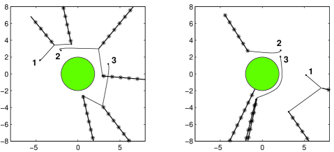
Figure 4: The solution to two instances of the RDTA problem using the branch and bound solver. The circle at the center of the field is the Defense Zone. The lines with asterisks denote the attacker trajectories, and the lines without denote defender trajectories. The parameters for these instances are $\epsilon=0.01$, $n=3$, and $m=6$.

In the remainder of this section we describe the components of the branch and bound solver in detail.

4.1 Node expansion

Here we describe the node expansion algorithm used to grow a search tree that enumerates all possible assignments for the RDTA problem. Each node of the tree represents an assignment. Starting from the root node, attackers are assigned, forming new nodes, until all complete assignments are generated. Each node represents a partial assignment except for the leaves, which represent the set of complete assignments.

Consider the case with one defender $\mathcal{D}=\{d_{1}\}$ and three attackers $\mathcal{A}=\{a_{1},a_{2},a_{3}\}$. The tree for this case is shown in Figure 5. To generate this tree, we start from the root node representing the empty assignment, denoted $\langle\rangle$. We expand the root node generating three children, each representing an assignment containing a single attacker to intercept. The children are then expanded, and so on, until all possible assignments are generated.

$\alpha_{d_{1}}=\langle\rangle$ $\langle a_{1}\rangle$ $\langle a_{1},a_{2}\rangle$ $\langle a_{1},a_{2},a_{3}\rangle$ $\langle a_{1},a_{3}\rangle$ $\langle a_{1},a_{3},a_{2}\rangle$ $\langle a_{2}\rangle$ $\langle a_{2},a_{1}\rangle$ $\langle a_{2},a_{1},a_{3}\rangle$ $\langle a_{2},a_{3}\rangle$ $\langle a_{2},a_{3},a_{1}\rangle$ $\langle a_{3}\rangle$ $\langle a_{3},a_{1}\rangle$ $\langle a_{3},a_{1},a_{2}\rangle$ $\langle a_{3},a_{2}\rangle$ $\langle a_{3},a_{2},a_{1}\rangle$

Figure 5: Search tree for the RDTA problem with the defender set $\mathcal{D}=\{d_{1}\}$ and the attacker set $\mathcal{A}=\{a_{1},a_{2},a_{3}\}$. Each node of the tree denotes a sequence of attackers to be intercepted by defender $d_{1}$. The root node is the empty assignment. The leaves of the tree give all possible complete assignments of attackers in $\mathcal{A}$.

For multiple defenders, unlike the single defender case, the tree is unbalanced to avoid redundancies. For example, consider the case with two defenders $\mathcal{D}=\{d_{1},d_{2}\}$ and two attackers $\mathcal{A}=\{a_{1},a_{2}\}$. The tree for this case is shown in Figure 6. Again, each node represents an assignment, but now the assignment is a sequence of attackers to intercept for each defender in $\mathcal{D}$.

$\begin{array}[]{c}\alpha_{d_{1}}=\langle\rangle\\ \alpha_{d_{2}}=\langle\rangle\end{array}$ $\begin{array}[]{c}\langle a_{1}\rangle\\ \langle\rangle\end{array}$ $\begin{array}[]{c}\langle a_{1},a_{2}\rangle\\ \langle\rangle\end{array}$ $\begin{array}[]{c}\langle a_{1}\rangle\\ \langle a_{2}\rangle\end{array}$ $\begin{array}[]{c}\langle a_{2}\rangle\\ \langle\rangle\end{array}$ $\begin{array}[]{c}\langle a_{2},a_{1}\rangle\\ \langle\rangle\end{array}$ $\begin{array}[]{c}\langle a_{2}\rangle\\ \langle a_{1}\rangle\end{array}$        $\begin{array}[]{c}\langle\rangle\\ \langle a_{1}\rangle\end{array}$ $\begin{array}[]{c}\langle\rangle\\ \langle a_{1},a_{2}\rangle\end{array}$        $\begin{array}[]{c}\langle\rangle\\ \langle a_{2}\rangle\end{array}$ $\begin{array}[]{c}\langle\rangle\\ \langle a_{2},a_{1}\rangle\end{array}$

Figure 6: Search tree for the RDTA problem with defender set $\mathcal{D}=\{d_{1},d_{2}\}$ and the attacker set $\mathcal{A}=\{a_{1},a_{2}\}$. Each node of the tree denotes a sequence of attackers to intercept for defender $d_{1}$ and defender $d_{2}$. The root node is the empty assignment. The leaves of the tree give all possible complete assignments of attackers in $\mathcal{A}$.

In general, for defender set $\mathcal{D}$ with $n$ defenders and attacker set $\mathcal{A}$ with $m$ attackers there are $(n+m-1)!/(n-1)!$ complete assignments (or leaves in the search tree).

To generate a search tree for the general case, we use a node expansion algorithm. This algorithm takes any node and generates the node’s children. The assignment for each child is constructed by appending an unassigned attacker to one of the sequences in the parent node’s assignment. The task sequences in the parent’s assignment are always subsequences of the sequences in its child’s assignment. Therefore, when we prune a node from the search tree, we can also prune all of its descendants.

The node expansion algorithm uses a different representation for an assignment than we have used thus far. We introduce this new representation with an example involving the defender set $\mathcal{D}=\{d_{1},d_{2}\}$ and the attacker set $\mathcal{A}=\{a_{1},a_{2},\ldots,a_{7}\}$. Consider a partial assignment given by

$$\alpha_{d_{1}}=\langle a_{4},a_{1}\rangle$$

$$\alpha_{d_{2}}=\langle a_{2},a_{5},a_{7}\rangle.$$

In this case, attackers $a_{3}$ and $a_{6}$ have yet to be assigned. Our node expansion algorithm represents this partial assignment with the vectors

$$\mathbf{\delta}=(1,1,2,2,2,0,0)$$

$$\mathbf{\beta}=(4,1,2,5,7,0,0),$$ (21)

both of length $m=7$. Vector $\mathbf{\delta}$ holds defender indices and vector $\mathbf{\beta}$ holds attacker indices. For a unique representation, the elements in $\mathbf{\delta}$ are ordered so that $\delta(i)\leq\delta(i+1)$. For the example case, attackers $a_{\beta(1)}$ and $a_{\beta(2)}$ (i.e., $a_{4}$ and $a_{1}$) are assigned to defender $d_{1}$ in sequence, and attackers $a_{\beta(3)}$, $a_{\beta(4)}$, $a_{\beta(5)}$ (i.e., $a_{2}$, $a_{5}$, $a_{7}$) are assigned to defender $d_{2}$ in sequence.

In general, the input to the node expansion algorithm is a parent node with assignment give by

$$\mbox{parent}.\mathbf{\delta}=(\delta(1),\delta(2),\ldots,\delta(p),0,\ldots,0)$$

$$\mbox{parent}.\mathbf{\beta}=(\beta(1),\beta(2),\ldots,\beta(p),0,\ldots,0),$$ (22)

where both vectors are of size $m$, and $p$ is the number of tasks already assigned (or the number of nonzero entries in each vector). The output is a set of $N_{child}$ children, where

$$N_{child}=(n-\delta(p)+1)(m-p).$$ (23)

Each child has assignment vectors $\mathbf{\delta}$ and $\mathbf{\beta}$ identical to its parent except for entries $\delta(p+1)$ and $\beta(p+1)$. In the child’s assignment, attacker $a_{\beta(p+1)}$ is appended to defender $d_{\delta(p+1)}$’s sequence of attackers to intercept $\alpha_{\delta(p+1)}$. The details of the node expansion algorithm are given in Table 3.

Table 3: Node expansion algorithm

1:   $k:=1$ 2:  for $i=\delta(p),\delta(p+1),\ldots,n$ do 3:     for each $j$ in the set $\{\{1,\ldots,m\}-\{\beta(1),\beta(2),\ldots,\beta(p)\}\}$  do 4:         $\mbox{child}(k).\mathbf{\delta}=\mbox{parent}.\mathbf{\delta}$ 5:         $\mbox{child}(k).\mathbf{\beta}=\mbox{parent}.\mathbf{\beta}$ 6:        $\mbox{child}(k).\delta(p+1)=i$ 7:        $\mbox{child}(k).\beta(p+1)=j$ 8:        $k:=k+1$ 9:     end for 10:  end for

To demonstrate the node expansion algorithm, we expand the node given by equation (21) as shown in Figure 8. Figure 8 shows the normal notation for this expansion.

$\begin{array}[]{c}\mathbf{\delta}=(1,1,2,2,2,0,0)\\ \mathbf{\beta}=(4,1,2,5,7,0,0)\end{array}$ $\begin{array}[]{c}\mathbf{\delta}=(1,1,2,2,2,2,0)\\ \mathbf{\beta}=(4,1,2,5,7,3,0)\end{array}$ $\begin{array}[]{c}\mathbf{\delta}=(1,1,2,2,2,2,0)\\ \mathbf{\beta}=(4,1,2,5,7,6,0)\end{array}$

Figure 7: The node from equation (21), written in node expansion format, is expanded using the node expansion algorithm in Table 3.

$\begin{array}[]{c}\alpha_{d_{1}}=\langle a_{4},a_{1}\rangle\\ \alpha_{d_{2}}=\langle a_{2},a_{5},a_{7}\rangle\end{array}$ $\begin{array}[]{c}\alpha_{d_{1}}=\langle a_{4},a_{1}\rangle\\ \alpha_{d_{2}}=\langle a_{2},a_{5},a_{7},a_{3}\rangle\end{array}$ $\begin{array}[]{c}\alpha_{d_{1}}=\langle a_{4},a_{1}\rangle\\ \alpha_{d_{2}}=\langle a_{2},a_{5},a_{7},a_{3},a_{6}\rangle\end{array}$

Figure 8: The expansion in Figure 8 in our original notation.

Using this algorithm, we can grow the assignment tree for any RDTA problem. In Figure 9 we show the tree for the two vehicle two attacker example written in our node expansion algorithm’s notation.

$\begin{array}[]{c}{\bf\delta}=(0,0)\\ {\bf\beta}=(0,0)\end{array}$ $\begin{array}[]{c}(1,0)\\ (1,0)\end{array}$ $\begin{array}[]{c}(1,1)\\ (1,2)\end{array}$ $\begin{array}[]{c}(1,2)\\ (1,2)\end{array}$ $\begin{array}[]{c}(1,0)\\ (2,0)\end{array}$ $\begin{array}[]{c}(1,1)\\ (2,1)\end{array}$ $\begin{array}[]{c}(1,2)\\ (2,1)\end{array}$         $\begin{array}[]{c}(2,0)\\ (1,0)\end{array}$ $\begin{array}[]{c}(2,2)\\ (1,2)\end{array}$         $\begin{array}[]{c}(2,0)\\ (2,0)\end{array}$ $\begin{array}[]{c}(2,2)\\ (2,1)\end{array}$

Figure 9: The tree from Figure 6 written using our node expansion algorithm’s notation.

4.2 Search algorithm

To determine the order in which we expand nodes, we have tried several tree search algorithms including the systematic search algorithms breadth first search (BFS), depth first search (DFS) [5], and A* search [35].

$n_{0}$ $n_{1}$ $n_{4}$ $n_{5}$ $n_{2}$ $n_{6}$ $n_{7}$ $n_{3}$ $n_{8}$ $n_{9}$

Figure 10: Example search tree used to illustrate the branching routine in the branch and bound solver.

The A* search algorithm orders nodes according to a heuristic branching function to help guide the search toward the optimal assignment. We use the upper bound algorithm presented in Section 4.3 as the branching function. The lower bound algorithm presented in Section 4.4 could also be used as the branching function.

For example, consider a tree with three levels, where node $i$ is labeled $n_{i}$ as shown in Figure 10. For this tree, BFS gives the ordering $(n_{0},n_{1},n_{2},n_{3},n_{4},n_{5},n_{6},n_{7},n_{8},n_{9})$, and DFS gives the ordering $(n_{0},n_{1},n_{4},n_{5},n_{2},n_{6},n_{7},n_{3},n_{8},n_{9})$. Suppose the upper bound algorithm run at each node $i$ gives the following results: $J_{ub}(n_{1})=3$, $J_{ub}(n_{2})=1$, $J_{ub}(n_{3})=2$, $J_{ub}(n_{4})=2$, $J_{ub}(n_{5})=1$, $J_{ub}(n_{6})=1$, $J_{ub}(n_{7})=1$, $J_{ub}(n_{8})=1$, $J_{ub}(n_{9})=0$. A* BFS gives the ordering $(n_{0},n_{2},n_{3},n_{1},n_{6},n_{7},n_{9},n_{8},n_{5},n_{4})$, and A* DFS gives the ordering $(n_{0},n_{2},n_{6},n_{7},n_{3},n_{9},n_{8},n_{1},n_{5},n_{4})$.

In A* search, the children of a node must be sorted with respect to the branching function. The maximum number of children that emanate from any given node is the $nm$ children emanating from the root node. Therefore, the maximum number of items that need to be sorted is $nm$. To sort the children, we use Shell’s method [29], which runs in $O((nm)^{3/2})$ time.

4.3 Upper bound algorithm

In this section, we describe a fast algorithm that generates a feasible complete assignment given any partial assignment. The cost of the resulting complete assignment is an upper bound on the optimal cost that can be achieved from the given partial assignment. The idea behind the upper bound algorithm is to assign unassigned attackers in a greedy way. At each step, we assign the attacker defender pair that results in the minimum intercept time. We proceed until all attackers are assigned or until none of the remaining attackers can be intercepted before entering the Defense Zone. The details of this algorithm, which runs in $O(nm^{2})$ time, are listed in Table 4.

The input to the algorithm is a partial assignment given by an intercept sequence $\alpha_{d}$ for each defender $d$ in $\mathcal{D}$ such that the set of unassigned attackers $\mathcal{A}_{u}$ is not empty. In addition, we take as inputs the variables associated with this partial assignment including the time for defender $d$ to complete its intercept sequence $\alpha_{d}$, given by $t_{d}(m_{d})$, and binary variable $\gamma_{a}$ for each $a$ in the set of assigned attackers $\mathcal{A}-\mathcal{A}_{u}$.

Given a partial assignment, the greedy step of the algorithm determines the attacker in the set $\mathcal{A}_{u}$ that can be intercepted in the minimum amount of time, denoted $a^{*}$. The corresponding defender that intercepts $a^{*}$ is denoted $d^{*}$. To determine this defender, attacker pair $(d^{*},a^{*})$ we form a matrix $C$ of intercept times. The matrix has size $|\mathcal{D}|\times|\mathcal{A}_{u}|$, and its elements are given by

$$c(d,a):=t_{d}(m_{d})+\Delta t_{int}(d,a,t_{d}(m_{d})),$$ (24)

for each $d$ in $\mathcal{D}$ and $a$ in $\mathcal{A}_{u}$. The element $c(d,a)$ is the time it would take defender $d$ to complete its intercept sequence $\alpha_{d}$ and then intercept attacker $a$. The minimum of these times gives the desired defender, attacker pair

$$c(d^{*},a^{*})=\min_{d\in\mathcal{D},a\in\mathcal{A}_{u}}c(d,a).$$ (25)

If $c(d^{*},a^{*})=\infty$, no attacker can be intercepted before it enters the Defense Zone. Thus, we set $\gamma_{a}:=1$ for each $a$ in $\mathcal{A}_{u}$. Then, we set $\mathcal{A}_{u}$ to the empty set because all attackers are effectively assigned, and we use equation (20) to calculate the upper bound $J_{ub}$. Otherwise, $c(d^{*},a^{*})$ is finite, and we add attacker $a^{*}$ to defender $d^{*}$’s intercept sequence by incrementing $m_{d^{*}}$ by one and setting $\alpha_{d^{*}}(m_{d^{*}}):=a^{*}$. Then, because $a^{*}$ has now been assigned, we remove it from the set of unassigned attackers by setting $\mathcal{A}_{u}:=\mathcal{A}_{u}-\{a^{*}\}$. If $\mathcal{A}_{u}$ is not empty, we have a new partial assignment, and we repeat the procedure. Otherwise, the assignment is complete and we use equation (20) to compute the upper bound $J_{ub}$.

Table 4: Greedy upper bound algorithm

1:  Given a partial assignment: intercept sequence $\alpha_{d}$ for each $d\in\mathcal{D}$, a nonempty set of unassigned attackers $\mathcal{A}_{u}$, $t_{d}(m_{d})$ for each $d\in\mathcal{D}$, and $\gamma_{a}$ for each $a\in(\mathcal{A}-\mathcal{A}_{u})$. 2:  Initialize variables for unassigned attackers. Set $\gamma_{a}:=0$ for each $a$ in $\mathcal{A}_{u}$. 3:  Calculate the elements of matrix $C$. For all $d\in\mathcal{D}$ and $a\in\mathcal{A}_{u}$, set $\displaystyle c(d,a):=t_{d}(m_{d})+\Delta t_{int}(d,a,t_{d}(m_{d})).$ 4:  while $\mathcal{A}_{u}$ not empty do 5:     Find minimum element of $C$ given by $\displaystyle c(d^{*},a^{*})=\min_{d\in\mathcal{D},a\in\mathcal{A}_{u}}c(d,a).$ 6:     If $c(d^{*},a^{*})=\infty$, no attacker in the set $\mathcal{A}_{u}$ can be intercepted before entering the Defense Zone. Break out of the while loop. 7:     Append attacker $a^{*}$ to defender $d^{*}$’s assignment by setting $m_{d^{*}}:=m_{d^{*}}+1$ and $\alpha_{d^{*}}(m_{d^{*}}):=a^{*}$. 8:     Update finishing time for $d^{*}$ by setting $t_{d^{*}}(m_{d^{*}}):=c(d^{*},a^{*})$. 9:     Remove $a^{*}$ from consideration since it has been assigned. Set $c(d,a^{*})$ to $\infty$ for all $d\in\mathcal{D}$, and set $\mathcal{A}_{u}:=\mathcal{A}_{u}-\{a^{*}\}$. 10:     Update matrix for defender $d^{*}$. For all attackers $a\in\mathcal{A}_{u}$, set $\displaystyle c(d^{*},a):=t_{d^{*}}(m_{d^{*}})+\Delta t_{int}(d^{*},a,t_{d^{*}}(m_{d^{*}})).$ 11:  end while 12:  For each $a$ in $\mathcal{A}_{u}$, set $\gamma_{a}:=1$. 13:  Set $\displaystyle J_{ub}:=\sum_{a\in\mathcal{A}}\gamma_{a}+\epsilon\max_{d\in\mathcal{D}}t_{d}(m_{d}).$

4.4 Lower bound algorithm

Here we describe a fast algorithm that generates a lower bound on the cost that can be achieved from any given partial assignment. The idea behind the algorithm is to use the principle of simultaneity. In assigning attackers from $\mathcal{A}_{u}$, we assume each defender can pursue multiple attackers simultaneously. The result is a potentially infeasible complete assignment because simultaneity is physically impossible. Because no feasible assignment can do better, the cost of this assignment is a lower bound on the optimal cost that can be achieved from the given partial assignment. The algorithm, which runs in $O(nm)$ time, is listed in Table 5.

Similar to the upper bound algorithm, the input to the lower bound algorithm is a partial assignment. This includes an intercept sequence $\alpha_{d}$ for each defender $d$ in $\mathcal{D}$ with $\mathcal{A}_{u}$ nonempty, $t_{d}(m_{d})$ for each defender $d$ in $\mathcal{D}$, and $\gamma_{a}$ for each attacker $a$ in $\mathcal{A}-\mathcal{A}_{u}$.

Each attacker $a$ in $\mathcal{A}_{u}$ is assigned a defender as follows: Form a matrix $C$ with elements

$$c(d,a):=t_{d}(m_{d})+\Delta t_{int}(d,a,t_{d}(m_{d})),$$ (26)

for all $d$ in $\mathcal{D}$ and $a$ in $\mathcal{A}_{u}$. Element $c(d,a)$ is equal to the time it takes $d$ to intercept the attackers in its intercept sequence $\alpha_{d}$ plus the time it would take to subsequently intercept attacker $a$. For each $a$ in $\mathcal{A}_{u}$, find the defender, denoted $d^{*}$, that can intercept $a$ in minimal time

$$c(d^{*},a)=\min_{d\in\mathcal{D}}c(d,a).$$ (27)

If $c(d^{*},a)=\infty$, we set $\gamma_{a}:=1$ because no defender can intercept attacker $a$ before it enters the Defense Zone. Otherwise, we set $\gamma_{a}:=0$ because defender $d^{*}$ can intercept attacker $a$ before it enters the Defense Zone. The lower bound is therefore give by

$$J_{lb}:=\sum_{a\in\mathcal{A}}\gamma_{a}+\epsilon\max_{\{a\in\mathcal{A}:\gamma_{a}=0\}}\left(\min_{d\in\mathcal{D}}c(d,a)\right).$$ (28)

Table 5: Lower bound algorithm

1:  Given a partial assignment: intercept sequence $\alpha_{d}$ for each $d\in\mathcal{D}$, a nonempty set of unassigned attackers $\mathcal{A}_{u}$, $t_{d}(m_{d})$ for each $d\in\mathcal{D}$, and $\gamma_{a}$ for each $a\in(\mathcal{A}-\mathcal{A}_{u})$. 2:  Calculate the elements of matrix $C$. For all $d\in\mathcal{D}$ and $a\in\mathcal{A}_{u}$, set $\displaystyle c(d,a):=t_{d}(m_{d})+\Delta t_{int}(d,a,t_{d}(m_{d})).$ 3:  for all $a\in\mathcal{A}_{u}$ do 4:     Find minimum element of $a$th column of $C$ given by $\displaystyle c(d^{*},a)=\min_{d\in\mathcal{D}}c(d,a).$ 5:     if $c(d^{*},a)=\infty$ then set $\gamma_{a}:=1$. 6:     else set $\gamma_{a}:=0$. 7:  end for 8:  Set $\displaystyle J_{lb}:=\sum_{a\in\mathcal{A}}\gamma_{a}+\epsilon\max_{\{a\in\mathcal{A}:\gamma_{a}=0\}}\left(\min_{d\in\mathcal{D}}c(d,a)\right).$

5 Analysis of the solver

In this section, we explore the average case computational complexity of the branch and bound algorithm by solving randomly generated instances. Each instance is generated by randomly selecting parameters from a uniform distribution over the intervals defined below. The computations were performed on a PC with Intel PIII 550MHz processor, 1024KB cache, 3.8GB RAM, and Linux. For all instances solved, processor speed was the limiting factor, not memory.

5.1 Generating random instances

The initial position of each attacker is taken to be in an annulus centered on the playing field. The radius of the initial position, denoted $r_{a}$, is chosen at random from a uniform distribution over the interval $[r_{a}^{\min},r_{a}^{\max}]$. The angle of the initial position, denoted $\theta_{a}$, is chosen from a uniform distribution over the interval $(0,2\pi]$ (all other angles used in this section $\phi_{a}$, $\theta_{d}$, and $\phi_{d}$ are also chosen from a uniform distribution over the interval $(0,2\pi]$). The magnitude of attacker $a$’s velocity, denoted $v_{a}$, is chosen at random from a uniform distribution over the interval $[v_{a}^{\min},v_{a}^{\max}]$. The initial state of the attacker is given by

$$p(0)=r_{a}\cos(\theta_{a}),\mbox{ }q(0)=r_{a}\sin(\theta_{a})$$

$$\dot{p}=v_{a}\cos(\phi_{a}),\mbox{ }\dot{q}=v_{a}\sin(\phi_{a}).$$ (29)

The initial position of each defender is taken to be in a smaller annulus, also centered on the playing field. The radius of the initial position, denoted $r_{d}$, is chosen at random from a uniform distribution over the interval $[r_{d}^{\min},r_{d}^{\max}]$. The magnitude of defender $d$’s velocity, denoted $v_{d}$, is chosen at random from a uniform distribution over the interval $[v_{d}^{\min},v_{d}^{\max}]$. The initial state of the defender is given by

$$x(0)=r_{d}\cos(\theta_{d}),\mbox{ }y(0)=r_{d}\sin(\theta_{d})$$

$$\dot{x}(0)=v_{d}\cos(\phi_{d}),\mbox{ }\dot{y}(0)=v_{d}\sin(\phi_{d}).$$ (30)

For the instances generated in this paper, we set $R_{dz}=2.0$ and take the parameters from the following intervals: $r_{a}\in[7.5,15.0]$, $v_{d}=1.0$, $r_{d}\in[\sqrt{2}R_{dz},2\sqrt{2}R_{dz}]$, and $v_{d}\in[0.5,1.0]$. In Section 5.3, we study the RDTA problem with variations in the velocity parameters $v_{a}$ and $v_{d}^{\max}$.

5.2 Average case computational complexity

In this section, we present the results of an average case computational complexity study on the branch and bound solver. A particular problem instance is considered solved when the strategy that minimizes the cost is found. In Figure 11, we plot the fraction of instances solved versus computation time. In the figure on top, the cost function is the number of attackers that enter the Defense Zone ($\epsilon=0$ in equation (20)). Solving these instances becomes computationally intensive for modest size problems. For example, when $n=3$ and $m=5$, 80% of the instances are solved in 60 seconds or less. In the figure on bottom, in addition to the primary component of the cost function, the cost function includes a secondary component ($\epsilon=0.01$ in equation (20)). The secondary component is the time it takes to intercept all attackers that can be intercepted. Solving these instances of the problem is more computationally intensive than the $\epsilon=0$ case. For example, when $n=3$ and $m=5$, only 40% of the problems are solved in 60 seconds or less.

Figure 11: The fraction of instances solved versus computation time for the branch and bound solver. On top, the cost is the number of attackers that enter the Defense Zone ($\epsilon=0$ in equation (20)), and on bottom, the cost includes a secondary component ($\epsilon=0.01$ in equation (20)). For each curve, 400 random instances of the RDTA problem were solved. The values of the parameters are $n=3$ and $m=3,4,5$.

The increase in average case computational complexity for the $\epsilon>0$ case is expected because the cost function has an additional component to be minimized, which is independent of the primary component. In a case where the primary component is at a minimum, the algorithm will proceed until it proves that the combination of primary and secondary components is minimized.

If it is given enough time, the branch and bound solver finds the optimal assignment, but the average case computational complexity is high. Therefore, using the algorithm to solve for the optimal assignment in real-time is infeasible for most applications. However, the best assignment found in the allotted time window for planning could be used in place of the optimal assignment. In this case, it is desirable that the algorithm converge to a near-optimal solution quickly.

To learn more about the convergence rate of the branch and bound solver, we look at the rate at which the best upper bound $J_{ub}^{best}$ decreases with branches taken in the search tree. Because the branch and bound algorithm is an exact method, $J_{ub}^{best}$ eventually converges to $J_{opt}$. We define the percent difference from optimal as follows: Let $J_{opt}^{(i)}$ be the optimal cost for instance $i$. Let $J_{ub}^{(i)}(k)$ be the best upper bound found after $k$ branches for instance $i$. Let $\hat{J}_{opt}$ be the mean of the set $\{J_{opt}^{(i)}:i=1,\ldots,N\}$, and let $\hat{J}_{ub}(k)$ be the mean of the set $\{J_{ub}^{(i)}(k):i=1,\ldots,N\}$, where $N$ is the number of instances. The percent difference from optimal is given by

$$\mbox{PD}(k)=100\frac{\hat{J}_{ub}(k)-\hat{J}_{opt}}{\hat{J}_{opt}}.$$ (31)

Figure 12: The average convergence rate for the branch and bound solver using each of the three branching routines BFS, DFS, and A* search. We plot the percent difference from optimal $\mbox{PD}(k)$ versus the number of branches $k$ explored. For each curve 400 random instances of RDTA were solved. The parameters values are $\epsilon=0.01$, $n=3$, and $m=5$.

In Figure 12, we plot PD$(k)$ versus the number of branches $(k)$ for instances involving three defenders ($n=3$) and five attackers ($m=5$). At the root node ($k=1$), the greedy algorithm is applied. Exploration of the tree does not occur at this point. Therefore, the three branching routines produce the same result, $\mbox{PD}(1)=33\%$. This means that $\hat{J}_{ub}(1)-\hat{J}_{opt}=0.33\hat{J}_{opt}$, or $\hat{J}_{ub}(1)=1.33\hat{J}_{opt}$. In other words, the average cost of the assignment generated by the greedy algorithm is 1.33 times the average optimal cost. At one branch into the tree ($k=2$), both DFS and BFS generate assignments with $\mbox{PD}(2)=28\%$, and the A* search generates assignments with $\mbox{PD}(2)=5\%$. Therefore, after only two steps, the branch and bound algorithm using A* search generates an assignment that, on average, has cost only 1.05 times the cost of the optimal assignment.

For the instances solved here, the branch and bound solver with A* search converges to the optimal assignment in an average of 8 branches, and it takes an average of 740 branches to prove that the assignment is optimal. Therefore, the solver converges to the optimal solution quickly, and the computational complexity that we observed (Figure 11) is due to the time needed to prove optimality.

These results are encouraging for real-time implementation of the algorithm. The results show that a very good assignment is generated after a short number of branches. There is a trade-off between optimality and computation time that can be tuned by deciding how deep into the tree to explore. Going deeper into the tree will generate assignments that are closer to optimal, but at the same time, results in an increased computational burden. The parameter to be tuned is the maximum number of branches to allow the search procedure to explore, denoted ${\tt kMax}$.

To study the computational complexity as ${\tt kMax}$ is tuned, we look at versions of the algorithm (using A*) with ${\tt kMax}=1$ (greedy algorithm), ${\tt kMax}=2$, and ${\tt kMax}=\infty$ (exact algorithm). These three cases generate assignments with average percent difference from optimal given by PD(1)=33%, PD(2)=5%, and PD($\infty$)=0% respectively. The results are shown in Figure 13. The algorithm with ${\tt kMax}=2$ gives a good balance between optimality and computation time.

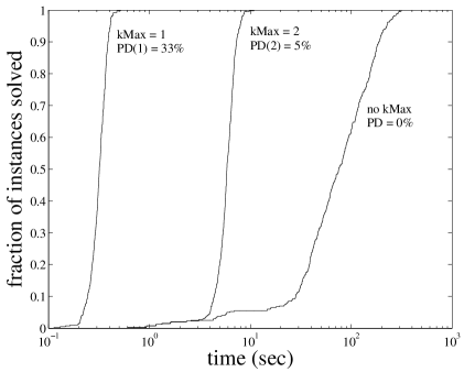
Figure 13: The fraction of instances solved versus computation time for the branch and bound solver (using A*) with ${\tt kMax}=1,2,\mbox{ and }\infty$. The ${\tt kMax}$ variable controls the maximum number of branches explored. We vary it from ${\tt kMax}=1$, which is a greedy search, to ${\tt kMax}=\infty$, which is exhaustive search. For each curve, 400 random instances of the RDTA problem was solved. For these problems the parameter values are $\epsilon=0.01$, $n=3$, and $m=5$.

5.3 Phase Transitions

The RDTA problem is NP-hard [14], which can be shown by reduction using the traveling salesman problem. This is a worst case result that says nothing about the average case complexity of the algorithm or the complexity with parameter variations. In this section, we study the complexity of the RDTA problem as parameters are varied. We perform this study on the decision version of the problem.

RoboFlag Drill Decision Problem (RDD): Given a set of defenders $\mathcal{D}$ and a set of attackers $\mathcal{A}$, is there a complete assignment such that no attacker enters the Defense Zone?

First, we consider variations in the ratio of attacker velocity to maximum defender velocity, denoted $vA/vD$ in this section. When the ratio is small, the defenders are much faster than the attackers. It should be easy to quickly find an assignment such that all attackers are intercepted. When the ratio is large, the attackers are much faster than the defenders. In this case, it is difficult for the defenders to intercept all of the attackers, which should be easy to determine.

The interesting question is whether there is a transition from being able to intercept all the attackers (all yes answers to the RDD problem) to not being able to intercept all attackers (all no answers to the RDD problem). Is this transition sharp? Are there values of the ratio for which solving the RDD is difficult?

For each value of the velocity ratio, we generated random instances of the RDD problem and solved them with the branch and bound solver. The results are shown in Figure 14. The figure on top shows the fraction of instances that evaluate to yes versus the velocity ratio. The figure on bottom shows the mean number of branches required to solve an instance versus the velocity ratio. There is a sharp transition from all instances yes to all instances no. This transition occurs approximately at $vA/vD=1$ for the $n=3$, $m=5$ case. At this value of the ratio, there is a spike in computational complexity. This easy-hard-easy behavior is indicative of a phase transition [2, 25].

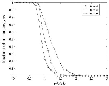
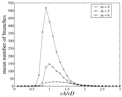
Figure 14: The phase transition of the RDD problem in the ratio of attacker velocity to maximum defender velocity ($vA/vD$). The figure on top shows the fraction of instances that evaluate to yes versus the velocity ratio. The figure on bottom shows the mean number of branches needed to solve the problem versus the velocity ratio. The phase transition occurs at a velocity ration of approximately 1. For each curve, 100 random instances of the RDD problem were solved. In these figures, $n=3$.

We also study the RDD problem with variations in the ratio of defenders to attackers, denoted $n/m$, with $vD=vA=1$. For small values of $n/m$, the number of attackers is much larger than the number of defenders, and it should be easy to determine that the team of defenders cannot intercept all of the attackers. In this case, most instances should evaluate to no. For large values of $n/m$, the number of defenders is much larger than the number of attackers, and it should be easy to find an assignment in which all attackers are denied from the Defense Zone. In this case, most instances should evaluate to yes. The results are shown in Figure 15, where it is clear that our expectations proved correct. In between the extremes of the $n/m$ ratio, there is a phase transition at a ratio of approximately $n/m=0.65$.

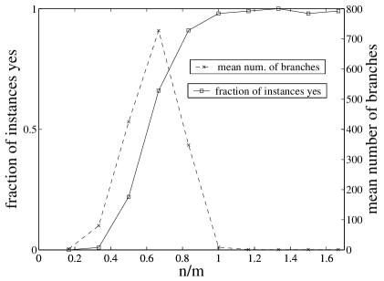
Figure 15: The phase transition of the RDD problem in the ratio of defenders to attackers ($n/m$). The solid line shows the fraction of instances that evaluate to yes versus the ratio. The dashed line shows the mean number of branches needed to solve the problem versus the ratio. For each curve, 100 random instances of the RDD problem were solved. The velocities are $vD=vA=1$.

In general, these experiments show that when one side dominates the other (in terms of the number of vehicles or in terms of the capabilities of the vehicles) the RDD problem is easy to solve. When the capabilities are comparable (similar numbers of vehicles, similar performance of the vehicles), the RDD is much harder to solve. This behavior is similar to the complexity of balanced games like chess [16]. In Section 7, we discuss how knowledge of the phase transition can be exploited to reduce computational complexity.

6 Multi-level implementation

Now that we have a fast solver that generates near-optimal assignments, we test it in a dynamically changing environment. We consider the RoboFlag Drill problem with attackers that have a simple noncooperative strategy built in, which is unknown to the defenders. The hope is that frequent replanning, at all levels of the hierarchical decomposition, will mitigate our assumption that the attackers move with constant velocity.

We use a multi-level receding horizon architecture, shown in Figure 16, to generate the defenders’ strategy. The task assignment module at the top level implements the branch and bound algorithm presented in this paper. It generates the assignment $\alpha_{d}$ for each defender $d$, sending new assignments to the middle level of the hierarchy at the rate $R_{TA}$. Therefore, the algorithm returns the best assignment computed in the time window $1/R_{TA}$.

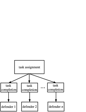
Figure 16: The multi-level architecture for the defending vehicles used in our implementation.

There is a task completion module for each defender at the middle level of the hierarchy, which receives an updated assignment $\alpha_{d}$ from the task assignment module at the rate $R_{TA}$. At a rate $R_{TC}$, the task completion module generates a trajectory from defender $d$’s current state to a point that will intercept attacker $\alpha_{d}(1)$ assuming the attacker moves at constant velocity. If attacker $\alpha_{d}(1)$ is intercepted, a trajectory to intercept attacker $\alpha_{d}(2)$ is generated, and so on.

The vehicle module at the bottom of the hierarchy receives an updated trajectory from the task completion module at the rate $R_{TC}$. The module propels the vehicle along this trajectory until it receives an update.

The attackers are taken to be the same vehicles as the defenders (described in Appendix A). For the attacker intelligence, we use the architecture shown in Figure 17. The levels of the hierarchy are decoupled, so each attacker acts independently. The simple intelligence for each attacker is contained in the top level of the hierarchy. The primary objective is to arrive at the origin of the field in minimum time. However, the attacker tries to avoid the defenders if they get too close. The radius of each defender is artificially enlarged by a factor $\beta>1$. If the artificially enlarged defenders obstruct an attacker’s path toward the origin, the attacker treats them as obstacles, finding a destination that results in an obstacle free path. The destination is found using a simple reactive obstacle avoidance routine used in RoboCup [6, 37]. The attacker intelligence module runs at the rate $R_{I}$.

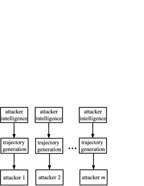
Figure 17: The multi-vehicle architecture for the attackers used to test the defender architecture.

The trajectory generation module at the middle of the hierarchy receives an updated destination at the rate $R_{I}$. The module generates a trajectory from the current state of the attacker to the destination with zero final velocity at the rate $R_{TG}$, using techniques from [27]. The vehicle module at the bottom level of the hierarchy is the same as that for the defenders.

Because the algorithms are more computationally intensive for the higher levels of the hierarchy than the lower levels, the rates are constrained as follows: $R_{TA}<R_{TC}$ and $R_{I}<R_{TG}$. In the simulations that follow, we take $R_{TC}=R_{TG}$ because the middle levels of the two hierarchies are comparative computationally. We also set $R_{I}=R_{TG}/10$. Therefore, if the trajectory generation module replans every time unit, the attacker intelligence module replans every ten time units.

First, note that when both $R_{TA}$ and $R_{TC}$ are zero, there is no replanning. In this case, all attackers usually enter the Defense Zone. They easily avoid the defenders because the defenders execute a fixed plan, which becomes obsolete once the attackers start using their intelligence.

Next, we present simulation results of the RoboFlag Drill with intelligent attackers and defenders. We consider problems with eight defenders ($n=8$), four attackers ($n=4$), $vA=vD$, $R_{TC}=R_{TG}>0$, and $R_{I}=R_{TG}/10$. We consider several different values of the rate at which the task assignment module replans ($R_{TA}$). For each value, we solve 200 randomly generated instances of the problem. As an evaluation metric, we use the average number of attackers that enter the Defense Zone during play.

For the case $R_{TA}=0$, there is no replanning at the task assignment level. Replanning only occurs at the task completion level. The defenders are given a plan from the task assignment module at the beginning of play. Each defender executes its assignment throughout, periodically recalculating the trajectory it must follow to intercept the next attacker in its sequence. For this case, on average, 58% of the attackers enter the Defense Zone during play.

For the case $R_{TA}>0$, replanning occurs at both the task assignment level and the task completion level of the hierarchy. In addition to recomputing trajectories to intercept the next attacker in each defender’s assignment, the defender assignments are recomputed. This redistributes tasks based on the current state of the dynamically changing environment, providing feedback. For $R_{TA}=R_{TC}/40$, $R_{TC}/20$, and $R_{TC}/15$, an average of 38%, 34%, and 32.5% of the attackers enter the Defense Zone during play, respectively. Therefore, replanning at the task assignment level has helped increase the utility of the strategies generated for the team of defenders.

In Figure 18, we show snapshots of an instance of the RoboFlag Drill simulation for the case where the defenders do not replan at the task assignment level. In this case, all attackers enter the Defense Zone. In Figure 19, we show snapshots of the same instance of the RoboFlag Drill simulation, but in this case, the defenders replan at the task assignment level ($R_{TA}=R_{TC}/15$). The defenders cooperate to deny all attackers from the Defense Zone. For example, the two defenders at the lower left of the field cooperate to intercept an attacker.

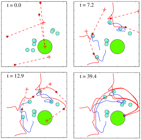
Figure 18: Snapshots of the RoboFlag Drill simulation with defender replanning at the task completion level only ($R_{TA}=0$). In this case, all attackers enter the Defense Zone. The large circles are the defenders, and the small circles are the attackers. The solid lines are trajectories. Each cross connected to a dashed line is an attacker’s desired destination.

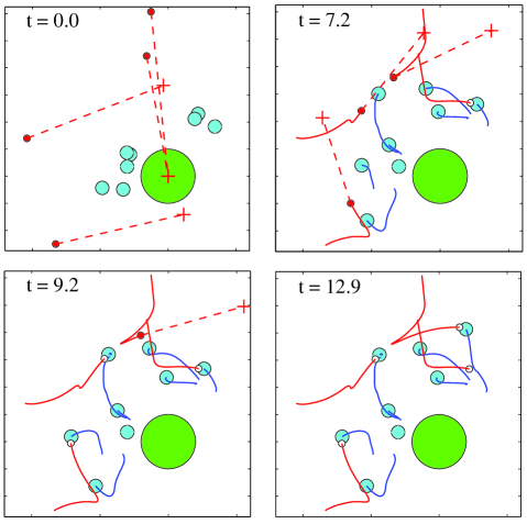
Figure 19: Snapshots of the RoboFlag Drill simulation with defender replanning at the task completion level and task assignment level ($R_{TA}=R_{TC}/15$). Because there is replanning at both levels, the defenders cooperate to intercept all attackers. The large circles are the defenders, and the small circles are the attackers. The solid lines are trajectories. Each cross connected to a dashed line is an attacker’s desired destination.

7 Discussion

We developed a decomposition approach that generates cooperative strategies for multi-vehicle control problems, and we motivated the approach using an adversarial game called RoboFlag. In the game, we fixed the strategy for one team and used our approach to generate strategies for the other team. By introducing a set of tasks to be completed by the team and a task completion method for each vehicle, we decomposed the problem into a high level task assignment problem and a low level task completion problem. We presented a branch and bound solver for task assignment, which uses upper and lower bounds on the optimal assignment to prune the search space. The upper bound algorithm is a greedy algorithm that generates feasible assignments. The best greedy assignment is stored in memory during the search, so the algorithm can be stopped at any point in the search and a feasible assignment is available.

In our computational complexity study, we found that solving the task assignment problem is computationally intensive, which was expected because the problem is NP-hard. However, we showed that the solver converges to the optimal assignment quickly, and takes much more time to prove the assignment is optimal. Therefore, the solver can be run in a time window to generate near-optimal assignments for real-time multi-vehicle strategy generation. To increase the speed of the algorithm, it may be advantageous to distribute the computation over the set of vehicles [30], taking advantage of the distributed structure of the problem.

We also studied the computational complexity of the solver as parameters were varied. We varied the ratio of the maximum velocities of the opposing vehicles, and we varied the ratio of the number of vehicles per team. We found that when one team has a capability advantage over the other, such as a higher maximum velocity or more vehicles, the solution to the task assignment problem is easy to generate. However, when the teams are comparable in capability, finding the optimal assignment to the problem is much more computationally intensive. This type of analysis can help in deciding how many vehicles to deploy in an adversarial game and what capabilities the vehicles should have. In addition, knowledge of the phase transition may be exploited to reduce computational complexity. In [31, 32], phase transition ‘backbones’ are exploited to decompose combinatorial problems into many separate subproblems, which are much less computationally intensive. This decomposition is amenable to parallel computation. In [15], it is shown that the hardness of a problem depends on the parameters of the problem (as we showed above) and the details of the algorithm used to solve the problem. Therefore, it is possible that the hard instances of our problem, which lie along the phase transition, may be solved faster if we use a different solution algorithm. The authors in [15] suggest adding randomization to the algorithm and using a rapid restart policy. The restart policy selects a new random seed for the algorithm and restarts it if the algorithm is not making sufficient progress with the current seed.

Finally, we demonstrated the effectiveness of our approach in an environment where the adversaries had a noncooperative intelligence that was unknown. We found that the simple model used for the adversaries in the solver could be mitigated by a multi-level replanning architecture. In this architecture, there are two levels: low level task completion and high level task assignment. When replanning does not occur at either level, the solver fails because it generates a plan that becomes obsolete as the adversaries use their intelligence. When replanning occurs at the task completion level, an assignment is generated once by the solver. As the adversaries use their intelligence, the task completion component is run periodically for each vehicle, generating a new trajectory to complete the tasks in the vehicle’s assignment. This was somewhat effective at handling the unknown intelligence. When replanning occurs at both levels, the task assignment component is run periodically in addition to the task completion component. We found this replanning architecture effective at retasking in the dynamically changing environment. It is advantageous to replan frequently, on average, but there are instances where replanning frequently is not advantageous. In these cases, the vehicles are retasked so frequently that their productivity is reduced. Therefore, it may be desirable to place a penalty on changing each vehicle’s current task.

In general, we feel the multi-level replanning approach is a natural way to handle multi-vehicle cooperative control problems. There are many different directions for further research, including the addition of a high level learning module to generate better models of the adversaries through experience [38].

Appendix A Vehicle Dynamics

The wheeled robots of Cornell’s RoboCup Team [37] are the defenders in the RoboFlag problems we consider in this paper. We state their governing equations and simplify them by restricting the allowable control inputs [27]. The result is a linear set of governing equations coupled by a nonlinear constraint on the control input. This procedure allows real-time calculation of many near-optimal trajectories and has been successfully used by Cornell’s RoboCup team [37, 27].

Each vehicle has a three-motor omni-directional drive which allows it to move along any direction irrespective of its orientation. This allows for superior maneuverability compared to traditional nonholonomic (car-like) vehicles. The nondimensional governing equations for each vehicle are given by

$$\left[\begin{array}[]{c}\ddot{x}(t)\\ \ddot{y}(t)\\ \ddot{\theta}(t)\end{array}\right]+\left[\begin{array}[]{c}\dot{x}(t)\\ \dot{y}(t)\\ \frac{2mL^{2}}{J}\dot{\theta}(t)\end{array}\right]=\mathbf{u}(\theta(t),t),$$ (32)

where $(x(t),y(t))$ are the coordinates of the robot on the playing field, $\theta(t)$ is the orientation of the robot, and $\mathbf{u}(\theta(t),t)=\mathbf{P}(\theta(t))\mathbf{U}(t)$ can be thought of as a $\theta(t)$-dependent control input, where

$$\mathbf{P}(\theta)=\left[\begin{array}[]{ccc}-\sin(\theta)&-\sin(\frac{\pi}{3}-\theta)&\sin(\frac{\pi}{3}+\theta)\\ \cos(\theta)&-\cos(\frac{\pi}{3}-\theta)&-\cos(\frac{\pi}{3}+\theta)\\ 1&1&1\end{array}\right],$$ (33)

and

$$\mathbf{U}(t)=\left[\begin{array}[]{c}U_{1}(t)\\ U_{2}(t)\\ U_{3}(t)\end{array}\right].$$ (34)

In the equations above, $m$ is the mass of the vehicle, $J$ is the vehicle’s moment of inertia, $L$ is the distance from the drive to the center of mass, and $U_{i}(t)$ is the voltage applied to motor $i$.

By restricting the admissible control inputs we simplify the governing equations in a way that allows near-optimal performance. The set of admissible voltages $\mathcal{U}$ is given by the unit cube and the set of admissible control inputs is given by $P(\theta)\mathcal{U}$. The restriction involves replacing the set $P(\theta)\mathcal{U}$ with the maximal $\theta$-independent set found by taking the intersection of all possible sets of admissible controls. This set is characterized by the inequalities

$$u_{x}(t)^{2}+u_{y}(t)^{2}\leq\left(\frac{3-|u_{\theta}(t)|}{2}\right)^{2}$$ (35)

and

$$|u_{\theta}(t)|\leq 3,$$ (36)

where the $\theta$-independent control is given by $(u_{x}(t),u_{y}(t),u_{z}(t))$. The equations of motion become

$$\left[\begin{array}[]{c}\ddot{x}(t)\\ \ddot{y}(t)\\ \ddot{\theta}(t)\end{array}\right]+\left[\begin{array}[]{c}\dot{x}(t)\\ \dot{y}(t)\\ \frac{2mL^{2}}{J}\dot{\theta}(t)\end{array}\right]=\left[\begin{array}[]{c}u_{x}(t)\\ u_{y}(t)\\ u_{\theta}(t)\end{array}\right],$$ (37)

subject to constraints (35) and (36), which couple the degrees of freedom. To decouple the $\theta$ dynamics we set $|u_{\theta}(t)|\leq 1$. Then constraint (35) becomes

$$u_{x}(t)^{2}+u_{y}(t)^{2}\leq 1.$$ (38)

Now the equations of motion for the translational dynamics of the vehicle are given by

$$\ddot{x}(t)+\dot{x}(t)=u_{x}(t)$$

$$\ddot{y}(t)+\dot{y}(t)=u_{y}(t),$$ (39)

subject to constraint (38). In state space form we have

$$\dot{\mathbf{x}}(t)=\mathbf{A}_{c}\mathbf{x}(t)+\mathbf{B}_{c}\mathbf{u}(t),$$ (40)

where $\mathbf{x}=(x,y,\dot{x},\dot{y})$ is the state and $\mathbf{u}=(u_{x},u_{y})$ is the control input.

References

- [1] R. W. Beard, T. W. McLain, M. A. Goodrich, and E.P. Anderson, “Coordinated Target Assignment and Intercept for Unmanned Air Vehicles,” IEEE Trans. Robot. Automat., vol. 18, pp. 991–922, Dec. 2002.
- [2] R. Bejar, I. Vetsikas, C. Gomes, Henry Kautz, and B. Selman, “Structure and Phase Transition Phenomena in the VTC Problem,” In TASK PI Meeting Workshop, 2001.
- [3] M. Campbell, R. D’Andrea, D. Schneider, A. Chaudhry, S. Waydo, J. Sullivan, J. Veverka, and A. Klochko, “RoboFlag Games using Systems Based, Hierarchical Control,” Proceedings of the American Control Conference, June 4–6, 2003, pp. 661–666.
- [4] C. G. Cassandras and W. Li, “A Receding Horizon Approach for Solving Some Cooperative Control Problems,” Proc. IEEE Conf. Decision and Control, Las Vegas, Neveda, Dec. 2002, pp. 3760–3765.
- [5] T. H. Cormen, C. E. Leiserson, R. L. Rivest, and C. Stein. Introduction to Algorithms. Second Edition. The MIT Press, Cambridge, Massachusetts, 2001.
- [6] R. D’Andrea, T. Kalmár-Nagy, P. Ganguly, and M. Babish, “The Cornell Robocup Team,” In G. Kraetzschmar, P. Stone, T. Balch Eds., Robot Soccer WorldCup IV, Lecture Notes in Artificial Intelligence, Springer, 2001.
- [7] R. D’Andrea and R. M. Murray, “The RoboFlag Competition,” Proceedings of the American Control Conference, June 4–6, 2003, pp. 650–655.
- [8] R. D’Andrea and M. Babish, “The RoboFlag Testbed,” Proceedings of the American Control Conference, June 4–6, 2003, pp. 656–660.
- [9] W. B. Dunbar and R. M. Murray, “Distributed Receding Horizon Control with Application to Multi-Vehicle Formation Stabilization,” Accepted to Automatica, June, 2004.
- [10] A web page that accompanies this paper can be found at http://control.mae.cornell.edu/earl/decomp
- [11] M. G. Earl and R. D’Andrea, “Multi-vehicle Cooperative Control Using Mixed Integer Linear Programming,” preprint available at http://control.mae.cornell.edu/earl/milp1
- [12] M. G. Earl and R. D’Andrea, “Iterative MILP Methods for Vehicle Control Problems,” Proc. IEEE Conf. Decision and Control, Atlantis, Paradise Island, Bahamas, Dec. 2004.
- [13] M. G. Earl and R. D’Andrea, “Modeling and Control of a Multi-agent System using Mixed Integer Linear Programming,” Proc. IEEE Conf. Decision and Control, Las Vegas, Neveda, Dec. 2002, pp. 107–111.
- [14] M. R. Garey and D. S. Johnson. Computers And Intractability: A guide to the Theory of NP-Completeness. W. H. Freeman and Company, 1979.
- [15] C. P. Gomes, B. Selman, N. Crato, and H. Kautz, “Heavy-tailed Phenomena in Satisfiability and Constraint Satisfaction Problems,” Journal of Automated Reasoning, 24 (1-2): 67–100 FEB 2000.
- [16] H. J. van den Herik, J. W. H. M. Uiterwijk, J. van Rjiswijck, “Games Solved: Now and in the Future,” ARTIFICIAL INTELLIGENCE vol. 134 (1-2): pp. 277-311, Jan. 2002.
- [17] Y. Ho and K. Chu, “Team Decision Theory and Information Structures in Optimal Control Problems – Part 1,” IEEE Trans. Automatic Control, vol. AC-17, pp. 15–22, 1972.
- [18] E. Klavins, “A Language for Modeling and Programming Cooperative Control Systems,” Proceedings of the International Conference on Robotics and Automation, 2004.
- [19] E. Klavins, 42nd IEEE Conference on Decision and Control, “A Formal Model of a Multi-Robot Control and Communication Task,” Maui, HI, December 2003.
- [20] S. Kirkpatrick and B. Selman, “Critical-behavior in the Satisfiability of Random Boolean Expressions,” Science, 264 (5163), 1297–1301, MAY 27, 1994.
- [21] J. R. Kok, M. T. J. Spaan, and N. Vlassis, “Non-communicative multi-robot coordination in dynamic environments,” Robotics and Autonomous Systems, 50 (2–3): 99–114, Feb. 28, 2005.
- [22] P. U. Lima, F. C. A. Groen, “Special issue on multi-robots in dynamic environments,” Robotics and Autonomous Systems, 50 (2–3): 81–83, Feb. 28, 2005.
- [23] D. Q. Mayne, J. B. Rawlings, C. V. Rao, and P. O. M. Scokaert, “Constrained Model Predictive Control: Stability and Optimality,” Automatica, vol. 36, pp. 789–814, 2000.
- [24] M. Di Marco, A. Garulli, A. Giannitrapani, A. Vicino, “Simultaneous Localization and Map Building for a Team of Cooperating Robots: A Set Membership Approach,” IEEE Transactions on Robotics and Automation, vol. 19 (2), pp. 238–249, Apr. 2003.
- [25] R. Monasson, R. Zecchina, S. Kirkpatrick, B. Selman, and L. Troyansky, “Determining Computational Complexity from Characteristic ’Phase Transitions’,” Nature, 400(8), 1999.
- [26] R. Murphey and P. M. Pardalos, Eds., Cooperative Control and Optimization, Boston: Kluwer Academic, 2002.
- [27] T. Kalmár-Nagy, R. D’Andrea, and P. Ganguly. “Near-Optimal Dynamic Trajectory Generation and Control of an Omnidirectional Vehicle,” Robotics and Autonomous Systems, vol. 46, pp. 47–64, 2004.
- [28] J. Ousingsawat and M. E. Campbell, “Establishing Optimal Trajectories for Multi-vehicle Reconnaissance,” AIAA Guidance, Navigation and Control Conference, 2004.
- [29] W. H. Press, B. P. Flannery, S. A. Teukolsky, and W. T. Vetterling, Numerical Recipes in C : The Art of Scientific Computing, Cambridge University Press, New York, 1992.
- [30] T. L. Ralphs, “Parallel Branch and Cut for Capacitated Vehicle Routing,” Parallel Computing, vol. 29(5), pp. 607–629, May 2003.
- [31] J. Schneider, C. Froschhammer, I. Morgenstern, T. Husslein, and J. M. Singer, ”Searching for Backbones—An Efficient Parallel Algorithm for the Traveling Salesman Problem,” Computer Physics Communications, 96 (2-3): 173–188 AUG 1996.
- [32] J. Schneider, ”Searching for Backbones—A High-performance Parallel Algorithm for Solving Combinatorial Optimization Problems,” Future Generation Computer Systems, 19 (1): 121–131 JAN 2003.
- [33] T. Schouwenaars, E. Feron, B. de Moor, and J. P. How, “Mixed Integer Programming for Multi-vehicle Path Planning,” European Control Conference, September 2001.
- [34] B. Selman and S. Kirkpatrick, “Critical Behavior in the Computational Cost of Satisfiability Testing,” Artificial Intelligence, 81(1-2):273–295, 1996.
- [35] M. Stefik. Introduction to Knowledge Systems. Morgan Kaufmann Publishers, Inc., San Francisco, California, 1995.
- [36] S. A. Stoeter, P. E. Rybski, K. N. Stubbs, C. P. McMillen, M. Gini, D. F. Hougen, and N. Papanikolopoulos, “A robot team for surveillance tasks: Design and architecture,” Robotics and Autonomous Systems, 40 (2–3): 173–183 Aug. 31, 2002.
- [37] P. Stone, M. Asada, T. Balch, R. D’Andrea, M. Fujita, B. Hengst, G. Kraetzschmar, P. Lima, N. Lau, H. Lund,D. Polani,P. Scerri, S. Tadokoro,T. Weigel, and G. Wyeth, “RoboCup-2000: The Fourth Robotic Soccer World Championships,” AI MAGAZINE, vol. 22(1), pp. 11–38, Spring 2001.
- [38] P. Stone and M. Veloso, “Multiagent Systems: A Survey from a Machine Learning Perspective,” Autonomous Robots, vol. 8, pp. 345–383, 2000.