Performance of Gaussian Signalling in Non Coherent Rayleigh Fading Channels

Abstract

The mutual information of a discrete time memoryless Rayleigh fading channel is considered, where neither the transmitter nor the receiver has the knowledge of the channel state information except the fading statistics. We present the mutual information of this channel in closed form when the input distribution is complex Gaussian, and derive a lower bound in terms of the capacity of the corresponding non fading channel and the capacity when the perfect channel state information is known at the receiver.

I INTRODUCTION

An independent and identically distributed (iid) Gaussian is the capacity achieving input distribution for additive white Gaussian noise (non-fading) channel, a Rayleigh fading channel when the Channel State Information (CSI) is perfectly known at the receiver, and when the CSI is known to both the transmitter and the receiver. However, when CSI is not known by neither the transmitter nor the receiver, the capacity achieving distribution is not Gaussian [1]. Therefore, it is of practical interest to find the achievable information rate of non coherent Rayleigh fading channels when the input distribution is complex Gaussian.

Fading channels have been studied in depth and a plethora of literature is available on the upper and lower achievable rates over the wireless media; refer [2], [3] for a summary. However, most of the results were presented under various channel models applying constraints for mathematical representations, and the availability of (CSI) at the transmitter and receiver.

The capacity of fading channels when the CSI is perfectly known at the receiver was investigated initially by Ericson [4], later by Lee [5], and Ozarow, Shamai and Wyner [6]. This capacity is calculated in an average sense due to the time varying nature of the signal to noise ratio (SNR). The fading channel with CSI at the receiver alone and at both the transmitter and the receiver was extensively studied in [7], [8].

The iid Rayleigh fading channel with no CSI was studied by Faycal [1], [9], where it was shown that the capacity achieving input distribution is discrete with finite number of mass points with new emerging points as SNR increases. These mass point distribution tends to be uniform as SNR approaches infinity, deviating much form that of a Gaussian. The non coherent time selective Rayleigh fading channel has been further investigated by Yingbin and Venugopal [10] and derived upper and lower bounds on the capacity at high SNR.

In this paper, we determine how the Gaussian input distribution can contribute in non coherent Rayleigh fading channel. We achieve this by expressing the mutual information in closed form using Gauss-Hermit Quadrature with a simple lower bound on it and subsequently identifying the maximum deviation of the actual capacity achieved with a discrete input in the presence of Gaussian input.

II SYSTEM MODEL

Consider the Rayleigh fading channel,

$$y={a}{x}+{n}$$ (1)

where $y$ is the complex channel output, $x$ is the complex channel input, $a$ and $n$ represent the fading and noise components associated with the channel. It is assumed that $a$ and $n$ are independent zero mean circular complex Gaussian random variables. Also assume that ${\sigma_{a}^{2}}/{2}$ and ${\sigma_{n}^{2}}/{2}$ are the equal variance of real and imaginary parts of the complex variables $a$ and $n$ respectively and the time index in (1) is omitted for simplicity. The random variables $a$, $x$, and $n$ are considered to be independent of each other. The input $x$ $\epsilon$ $X$ is average power limited: $E[|x|^{2}]=\Omega_{x}^{2}\leq P$. The constant $\gamma=-\int_{0}^{\infty}{e^{-y}}{\log{y}}{dy}\approx 0.5772...,$  denotes the Euler’s constant. All the differential entropies and the mutual information are defined to the base “e”, and the results are expressed in “nats”. It is assumed that neither the receiver nor the transmitter has the knowledge of channel state information other than the statistics.

III THE MUTUAL INFORMATION

The Mutual information between the input and output of a Rayleigh fading channel can be expressed as [11]

$$I(X;Y) =\int_{0}^{\infty}{\int_{0}^{\infty}}{p_{Y|X}(y|x)}{p_{X}(x)}$$

$${\times}\,\,{\log\left[{\frac{p_{Y|X}(y|x)}{\int_{0}^{\infty}{p_{Y|V}(y|v)}{p_{V}(v)}{dv}}}\right]}\,{dx}{dy}$$ (2)

considering the probability distribution of the magnitudes of the input and output random variables $X$ and $Y$. It should be noted here that since we only consider the distribution of magnitudes of the random variables, the integral in (2) is taken from $0$ to ${\infty}$. The conditional probability density function (pdf) $p_{Y|X}(y|x)$ [9][11] is given by

$$p_{Y|X}(y|x)=\frac{2{|y|}}{{\sigma_{n}^{2}}+{\sigma_{a}^{2}}{|x|^{2}}}{\exp\left({\frac{-|y|^{2}}{{\sigma_{n}^{2}}+{\sigma_{a}^{2}}{|x|^{2}}}}\right)}.$$ (3)

Assume the average mean squared power of both fading $A$, ($a$ $\epsilon$ $A$) and noise $N$, ($n$ $\epsilon$ $N$) are unity. This assumption is valid since the effective received power at the receiver is the combination of both $\sigma_{a}^{2}$ and $\Omega_{x}^{2}$ and the SNR is the ratio between the average received power and the average noise power. Therefore, the same output exists for various $\sigma_{a}^{2}$ and $\sigma_{n}^{2}$ on the appropriate selection of $\Omega_{x}^{2}$. With this assumption, (3) can be written as

$$p_{Y|X}(y|x)=\frac{2{y}}{1+x^{2}}{\exp\left({\frac{-y^{2}}{1+x^{2}}}\right)}.$$ (4)

Without loss of generality, the magnitude sign is removed in (4) and the same notation will be used throughout the rest of this paper.

The mutual information [12] in (2) can be simplified to

$$I(X;Y) =h(Y)-h(Y|X)$$ (5a)

$$=-\int_{0}^{\infty}{p_{Y}(y){\log{p_{Y}(y)}}}{dy}$$

$$-\frac{1}{2}{\int_{0}^{\infty}{p_{X}(x)}{\log(1+x^{2})}{dx}}+{\log{2}}-({1+\frac{\gamma}{2}})$$ (5b)

where the first term in (5) is the channel output entropy $h(Y)$. This was originally proven by Taricco [11] deriving an analytical expression for the channel capacity using Lagrange optimization method with an additional constraint.

IV GAUSSIAN INPUT IN NON COHERENT RAYLEIGH FADING

Recall the channel model (1), and assume the input distribution is Gaussian. Then the distribution of both the real and imaginary parts of $x$ are independent and Gaussian. Therefore, the distribution of the $|x|$ is Rayleigh with the pdf [13]

$$p_{X}{(x)}={\frac{2{x}}{\Omega_{x}^{2}}}{\exp\left({\frac{-x^{2}}{\Omega_{x}^{2}}}\right)},\,x\geq 0.$$ (6)

It is assumed that both the real and imaginary parts of input have equal variance ${\Omega_{x}^{2}}/{2}$. The magnitude sign is omitted in (6) as mentioned in the previous section.

IV-A Output Conditional Entropy

Having described the input distribution $p_{X}(x)$ for non coherent Gaussian input channel, we now focus on the output conditional entropy $h(Y|X)$ in (5). By substituting (6) in (5) (except the first term described as $h(Y)$), we have

$$h(Y|X) ={\int_{0}^{\infty}\left[{\frac{{x}}{\Omega_{x}^{2}}{\exp\left({\frac{-x^{2}}{\Omega_{x}^{2}}}\right)}}{\log(1+x^{2})}\right]{dx}}$$

$$-{\log{2}}+({1+\frac{\gamma}{2}}).$$ (7)

With the detailed proof provided in Appendix A, we can reduce (7) to

$$h(Y|X)={-}\frac{1}{2}{\exp\left({\frac{1}{\Omega_{x}^{2}}}\right)}{\mathrm{Ei}\left(\frac{-1}{\Omega_{x}^{2}}\right)}-{\log{2}}+({1+\frac{\gamma}{2}}),$$ (8)

where the exponential integral $\mathrm{Ei}(x)={-}{\int_{-x}^{\infty}}{{e^{-t}}/{t}}\,{dt}$. Note that the channel capacity when the CSI is perfectly known at the receiver is [2], [4], [5],

$$C_{\text{rcsi}}=-{\exp\left({\frac{1}{snr}}\right)}{\mathrm{Ei}\left(\frac{-1}{snr}\right)},$$ (9)

where $snr=\Omega_{x}^{2}$ since $\sigma_{n}^{2}=1$. Therefore, $h(Y|X)$ in non coherent Rayleigh fading with Gaussian input can be expressed as

$$h(Y|X)=\frac{1}{2}{C_{\text{rcsi}}}-{\log{2}}+({1+\frac{\gamma}{2}}).$$ (10)

IV-B Output Entropy

The output pdf $p_{Y}(y)=\int_{0}^{\infty}{p_{X}(x)}{p_{Y|X}(y|x)}{dx}$ for the Gaussian input can be written as

$$p_{Y}(y)=\int_{0}^{\infty}{\frac{{2}{x}}{\Omega_{x}^{2}}}{\exp\left({\frac{-x^{2}}{\Omega_{x}^{2}}}\right)}\frac{2{y}}{1+x^{2}}{\exp\left({\frac{-y^{2}}{1+x^{2}}}\right)}{dx}.$$ (11)

Substituting (11) in the first term of (5) gives

$$h(Y) =-\int_{0}^{\infty}\int_{0}^{\infty}{\frac{{4}{x}{y}}{{\Omega_{x}^{2}}{(1+x^{2})}}}{\exp\left({-}{\frac{x^{2}}{\Omega_{x}^{2}}}-{\frac{y^{2}}{1+x^{2}}}\right)}{dx}$$

$${\times}\,{\log{\left[\int_{0}^{\infty}{\frac{{4}{x}{y}}{{\Omega_{x}^{2}}(1+x^{2})}}{\exp\left({-}{\frac{x^{2}}{\Omega_{x}^{2}}}-{\frac{y^{2}}{1+x^{2}}}\right)}{dx}\right]}}{dy}.$$ (12)

To the best of our knowledge, this integral can not be evaluated analytically $\forall\,\,\Omega_{x}^{2}$. In the following section we show the use of Gauss-Hermit polynomials to drive a closed form expression.

IV-C Gaussian Quadrature and Hermit Polynomials

A common method for approximating a definite integral is $\int_{a}^{b}{\omega(x)}{f(x)}{d{x}}\simeq\sum_{i=1}^{q}{A_{i}{f(x_{i})}}$, which is called Gauss-quadrature assuming the moments are defined and finite or bounded of the function ${\omega(x)}$ [14]. The Gaussian quadrature formula has a degree of precision or exactness $m$ if the solution is exact whenever $f(x)$ is a polynomial of degree $\leq m$ or equivalently, whenever $f(x)=\{1,x,....,x^{m}\}$ and it is not exact for $f(x)=x^{m+1}$. The $x_{i}$ are called the nodes of the formula and $A_{i}$ are called coefficients (or weights). If $\omega(x)$ is non negative in $[a,b]$, then $n$ points and coefficients can be found to make the solution exact for all polynomials of degree $\leq 2{q}-1$ and it is the highest degree of precision which can be obtained using $q$ points [14].

If the $\omega(x)$ is in the form of $e^{-x^{2}}$, the solution to the integral can be found using the roots (nodes) of the Hermit polynomial $H_{q}(x)$ [15] and the weights are given by

$$\omega_{i}=\frac{{2^{q-1}}{q!}{\sqrt{\pi}}}{{q^{2}}{\left[H_{q-1}(x_{i})\right]^{2}}}.$$

The roots and the weights are excessively given in [15] for $a=0$ and $b=\infty$ with $q=15$.

IV-D Output entropy $h(Y)$ in Closed form

Define $t^{2}=x^{2}/\Omega_{x}$, where $dx={\Omega_{x}}{dt}$, then substitution into (11) gives

$$p_{Y}(y)=\int_{t=0}^{t=\infty}{e^{-t^{2}}{\frac{{2}{t}{y}}{(1+{\Omega_{x}}{x^{2}})}{\exp\left[{\frac{-y^{2}}{2(1+{\Omega_{x}}{x^{2}})}}\right]}{dt}}}.$$ (13)

This integral is in the form of $\int_{a}^{b}{\phi}(v){\omega}(v){dv}$ where $\omega(v)\equiv{e^{-t^{2}}}$. Therefore it can be evaluated using Hermit polynomials in the form of $p_{Y}(y)=\sum_{j=1}^{q}{\omega_{j}}{f(v_{j})}$. The quantities $v_{j}$ and $\omega_{j}$ are the roots and the weights of the Hermit polynomials respectively. Applying these weights and roots in (13) we get

$$p_{Y}(y)=\sum_{j=1}^{q}{\omega_{j}}{\frac{{2}{v_{j}}{y}}{(1+{\Omega_{x}}{v_{j}^{2}})}}{\exp\left[{\frac{-y^{2}}{2(1+{\Omega_{x}}{v_{j}^{2}})}}\right]}.$$ (14)

Using this result, the output entropy $h(Y)$ can be written as

$$h(Y) =-\int_{0}^{\infty}\left\{\sum_{\ell=1}^{q}{\omega_{\ell}}{\frac{{2}{v_{\ell}}{y}}{(1+{\Omega_{x}}{v_{\ell}^{2}})}}{\exp\left[{\frac{-y^{2}}{2(1+{\Omega_{x}}{v_{\ell}^{2}})}}\right]}\right\}$$

$${\times}\,{\log}{\left\{\sum_{j=1}^{q}{\omega_{j}}{\frac{{2}{v_{j}}{y}}{(1+{\Omega_{x}}{v_{j}^{2}})}}{\exp\left[{\frac{-y^{2}}{2(1+{\Omega_{x}}{v_{j}^{2}})}}\right]}\right\}}{dy}.$$ (15)

Taking the integration inside and substituting $t^{2}=y^{2}/[2(1+\Omega_{x}v_{j}^{2})]$ in (15), the $\ell^{th}$ term where $\ell=1,....,q$ can be written as

$$h(Y)_{\ell}= -\int_{0}^{\infty}{e^{-t^{2}}}({4}{\omega_{l}}{v_{\ell}}{t})\log\left\{\sum_{j=1}^{q}{\frac{2{\sqrt{2}}{\omega_{j}}{v_{j}}{t}}{(1+\Omega_{x}{v_{j}^{2}})}}\right.$$

$$\left.{\times}\,{\sqrt{(1+\Omega_{x}{v_{\ell}^{2}})}}\,{\exp\left[{{-t^{2}}\frac{(1+\Omega_{x}{v_{\ell}^{2}})}{(1+\Omega_{x}{v_{j}^{2}})}}\right]}\right\}{dt}.$$ (16)

The integral in this $l^{th}$ term has the form of $\int_{a}^{b}{\phi}(v){\omega}(v){dv}$ where $\omega(v)\equiv{e^{-t^{2}}}$. We can now simplify (16) using Hermit polynomials as

$$h(Y)_{\ell} =\sum_{i=1}^{r}{\omega_{i}}({4}{\omega_{\ell}}{v_{\ell}}{v_{i}})\log\left\{\sum_{j=1}^{q}{\frac{2{\sqrt{2}}{\omega_{j}}{v_{j}}{v_{i}}}{(1+\Omega_{x}{v_{j}^{2}})}}\right.$$

$$\left.{\times}\,{\sqrt{(1+\Omega_{x}{v_{\ell}^{2}})}}\,{\exp\left[{{-v_{i}^{2}}\frac{(1+\Omega_{x}{v_{\ell}^{2}})}{(1+\Omega_{x}{v_{j}^{2}})}}\right]}\right\}.$$ (17)

The output entropy $h(Y)=-\sum_{\ell=1}^{q}{h(Y)_{\ell}}$ can be shown as

$$h(Y) =-\sum_{\ell=1}^{q}\sum_{i=1}^{r}({4}{\omega_{i}}{v_{i}}{\omega_{\ell}}{v_{\ell}})\log\left\{\sum_{j=1}^{q}{\frac{2{\sqrt{2}}{\omega_{j}}{v_{j}}{v_{i}}}{(1+\Omega_{x}{v_{j}^{2}})}}\right.$$

$$\left.{\times}\,{\sqrt{(1+\Omega_{x}{v_{\ell}^{2}})}}\,{\exp\left[{{-v_{i}^{2}}\frac{(1+\Omega_{x}{v_{\ell}^{2}})}{(1+\Omega_{x}{v_{j}^{2}})}}\right]}\right\}.$$ (18)

The $h(Y)$ presented in the closed form in (18) using Gauss-Hermit quadrature is very useful in finding the mutual information for any SNR and the computational time is much less than the numerical integrations to be carried out with high accuracy. The mutual information can be found subtracting (10) from (18). Fig. 1 depicts the mutual information obtained using the Gauss-Hermit polynomial method with the channel capacity [1].

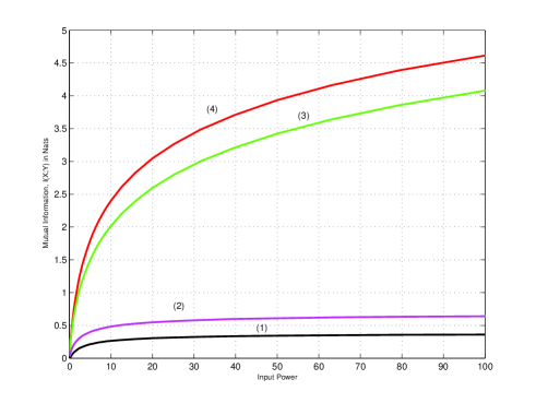
Figure 1: The mutual information with Gaussian input is below the channel capacity achieved by a discrete input. (1) The mutual information with gaussian input. (2) The channel capacity with a discrete input. (3) The channel capacity, $C_{\text{rcsi}}$ with CSI. (4) The non fading channel capacity, $C_{\text{cnf}}$.

Since the closed form expression obtained in the previous section is intricate with no straightforward or easy method to attain the result, we will show how to derive an analytical lower bound for (2) when the input is Gaussian distributed to understand its performance in a simplistic manner.

IV-E Lower Bound on Mutual Information

We have the following result.

Proposition 4.5.1:  The mutual information of an iid non coherent Rayleigh fading channel when the input distribution is complex Gaussian, is lower bounded by

$$I(X;Y)\geq\frac{1}{2}(C_{\text{cnf}}-C_{\text{rcsi}})$$ (19)

where $C_{\text{cnf}}$ and $C_{\text{rcsi}}$ are the capacity of the non fading complex Gaussian channel and the capacity of the Rayleigh fading channel when the CSI is perfectly known at the receiver. The equality holds when the average input power is zero.

Proof: We consider $I(X;Y)$, $h(Y)$, and $h(Y|X)$ when the input power $\Omega_{x}^{2}$ is zero. Using (8), we get $h(Y|X)_{\Omega_{x}^{2}=0}=-{\log{2}}+({1+\frac{\gamma}{2}})$. Since the mutual information is zero with no channel input, we can write

$$h(Y)_{\Omega_{x}^{2}=0}=h(Y|X)_{\Omega_{x}^{2}=0}.$$ (20)

The quantity $h(Y)$ in (12) is monotonically increasing with SNR, thus it has the minimum

$$h(Y)_{\text{min}}=-{\log{2}}+({1+\frac{\gamma}{2}}).$$ (21)

Consider, a non fading channel whose capacity achieving distribution is Gaussian, where $h(Y|X)_{\text{nf}}=h(N)=\frac{1}{2}{\log({\pi}{e}{\sigma_{n}^{2}})}$ is constant over input power. The monotonic increase of $h(Y)_{\text{nf}}=\frac{1}{2}{\log[{\pi}{e}{(\sigma_{n}^{2}+\Omega_{x}^{2})}]}$ with SNR results in significant increase in channel capacity.

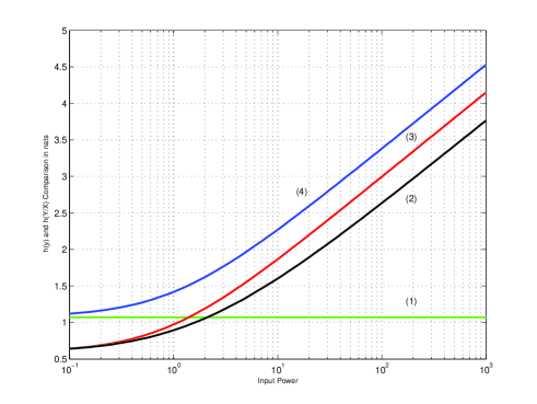
Figure 2: Entropy Comparison with Fading and Non fading Models: (1) Output conditional entropy of non fading channel, $h_{\text{nf}}(Y|X)$. (2) Output conditional entropy of fading channel with Gaussian input. (3) Output entropy of fading channel, $h(Y)$. (4) Output entropy of non fading channel, $h(Y)_{\text{{nf}}}$. The $h(Y)_{\text{{nf}}}$ and $h(Y)$ treated in this paper have a similar shape and the difference is decreasing with SNR.

The fading introduces the monotonic increase of output conditional entropy with SNR. In our investigation, we compare the differential output entropies in both cases and use the properties of the mutual information such as monotonic and non decreasing in order to draw a lower bound. We consider a single dimension of the non fading channel where the input and noise are complex random variables and hence both the output and the conditional entropies are taken accordingly. Fig. 2 portrays $h(Y)$ and $h(Y|X)$ of the two channel models, where

$$h(Y)_{\text{nf}}=\frac{1}{2}{\log[{\pi}{e}{(1+\Omega_{x}^{2})}]}$$ (22)

and

$$h(Y|X)_{\text{nf}}=\frac{1}{2}{\log({\pi}{e})}.$$ (23)

Note that the abbreviation “nf” refers the Gaussian channel with no fading present. Since the Gaussian distributions are the entropy maximisers for a power limited input,

$$h(Y)_{\text{nf}}>h(Y)\,\,\forall\,\,\Omega_{x}^{2}.$$ (24)

Lets define the difference in (24)

$$G=h(Y)_{\text{nf}}-h(Y),$$ (25)

and investigate the bounds when $\Omega_{x}^{2}=0$ and $\Omega_{x}^{2}\rightarrow\infty$. The $G_{\Omega_{x}^{2}=0}$ can be written as

$$G_{\Omega_{x}^{2}=0} =h(Y)_{nf,\Omega_{x}^{2}=0}-h(Y)_{\text{min}}$$

$$=\frac{1}{2}{\log({\pi}{e})}+{\log{2}}-({1+\frac{\gamma}{2}}).$$ (26)

To calculate the difference when $\Omega_{x}^{2}\rightarrow\infty$, we will use the upper bound

$${\lim\atop{\Omega_{x}^{2}\to\infty}}{I(X;Y)}\leq{\gamma}$$ (27)

given in [16]. Using (10) and (12), we can write the mutual information of the channel as

$$I(X;Y)=h(Y)-\frac{1}{2}{C_{\text{rcsi}}}+{\log{2}}-({1+\frac{\gamma}{2}}).$$ (28)

Substituting (27) and (28) in (25), we get,

$$G_{\Omega_{x}^{2}\rightarrow\infty} \geq\frac{1}{2}\,{\lim\atop{\Omega_{x}^{2}\to\infty}}\left\{{\log[{\pi}{e}{(1+\Omega_{x}^{2})}]}\right.$$

$$\left.+\,{\exp\left({\frac{1}{\Omega_{x}^{2}}}\right)}{\mathrm{Ei}\left(\frac{-1}{\Omega_{x}^{2}}\right)}\right\}-\gamma+{\log{2}}-({1+\frac{\gamma}{2}})$$

$$=L-\gamma+{\log{2}}-({1+\frac{\gamma}{2}}),$$ (29)

where $L=\frac{1}{2}[\gamma+\log({\pi}{e})]$. Refer the Appendix B for the detailed proof. Therefore we can write (IV-E) as,

$$G_{\Omega_{x}^{2}\rightarrow\infty}\geq\log({2}{\sqrt{{\pi}{e}}})-(1+\gamma).$$ (30)

Note that $G_{\Omega_{x}^{2}=0}>G_{\Omega_{x}^{2}\rightarrow\infty}$. The differential entropies defined in here are monotonic and concave with $\Omega_{x}^{2}$. The gap defined in (25) is the difference between two monotonic concave functions which would not necessarily be monotonic and concave. However, since $G_{\Omega_{x}^{2}=0}$ is higher than $G_{\Omega_{x}^{2}\rightarrow\infty}$, the quantity $G$ for any $\Omega_{x}^{2}$ should be less than $G_{\Omega_{x}^{2}=0}$ due to the properties of the two entropies mentioned. Therefore we conclude that the maximum difference occurs at $\Omega_{x}^{2}=0$. This $G_{\text{max}}=G_{\Omega_{x}^{2}=0}$ can be used to lower bound $h(Y)$ in (12) and we get

$$h(Y)\geq h(Y)_{\text{nf}}-G_{\text{max}}.$$ (31)

Therefore, the mutual information in (28) can be lower bounded as

$$I(X;Y) \geq h(Y)_{\text{nf}}-G_{\text{max}}-\left[\frac{1}{2}{C_{\text{rcsi}}}-{\log{2}}+({1+\frac{\gamma}{2}})\right]$$

$$=h(Y)_{\text{nf}}-\frac{1}{2}{\log({\pi}{e})}-\frac{1}{2}{C_{\text{rcsi}}}$$

$$=\frac{1}{2}{\log{(1+\Omega_{x}^{2})}}-\frac{1}{2}{C_{\text{rcsi}}},$$ (32)

using (10), (22), and (IV-E). With $C_{\text{cnf}}={\log{(1+\Omega_{x}^{2})}}$, we prove (19).
It should be noted here that (19) asymptotically converges to ${\gamma}/{2}$ since ${{\lim}\atop{{\Omega_{x}^{2}}_{\to}\infty}}(C_{\text{cnf}}-C_{\text{rcsi}})={\gamma}$ [16].

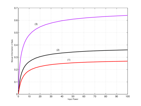
Figure 3: Analysis of the lower bound in fading channel: (1) The lower bound with Gaussian input. (2) The mutual information acquired using the closed form expression with Gauss-Hermit quadrature. (3) The channel capacity achieved with a discrete input.

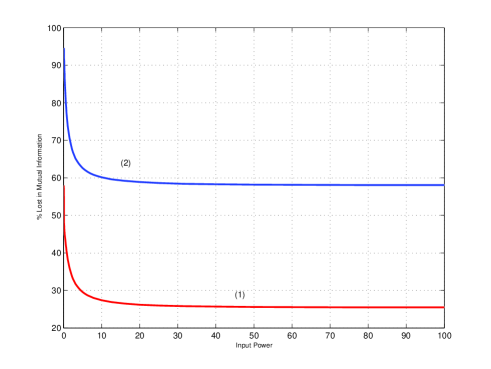
Figure 4: Percentage lost using the lower bound: (1) With the mutual information found numerically for Gaussian input. (2) With the channel capacity.

V NUMERICAL RESULTS

We compare the new lower bound with the mutual information found with the closed form expression attained through Gauss-Hermit quadrature in the previous section.

The lower bound in (19) is plotted against the input power in Fig. 3 with the mutual information obtained using the closed form expression. Further, it is compared with channel capacity acquired with discrete input [1]. The channel capacity is plotted for comparison only with two discrete mass points one located at the origin since the probability of other mass points are small at low SNR and even suited for a simple comparison at high SNR due to the percentage increase in capacity is low [9]. The percentage lost in mutual information with a Gaussian input on our lower bound is plotted in Fig. 4 where it shows $30\%$ less than the numerical values.

VI CONCLUSIONS

The mutual information of a non-coherent Rayleigh fading channel when the input is Gaussian distributed can be expressed in closed form using Gauss-Hermit quadrature. Further it can be lower bounded as the difference between the capacities of non fading channel and the Rayleigh fading channel when the perfect channel state information is known at the receiver. Even the Gaussian input is not optimal, our result shows the minimum achievable information rate which can be used as the worse case scenario in non coherent Rayleigh fading channels. The lower bound found is never lower than $70\%$ of the actual.

The CSI is obtained by training with known pilot symbols inserted in the transmitted sequence. Due to the presence of noise or under the fast fading conditions, the receiver is provided with imperfect CSI and the performance of the channel depends on its quality. Considering the worst case scenario, the channel can become non coherent with Gaussian input which optimises the mutual information with perfect CSI. Therefore, the closed form expression shown in this paper could be used as the lower bound with the imperfect CSI at the receiver.

VII APPENDIX

VII-A PROOF OF CONDITIONAL ENTROPY IN (8)

We write (7) as

$$h(Y|X)=E_{1}-{\log{2}}+({1+\frac{\gamma}{2}})$$ (33)

where

$$E_{1}={{\lim}\atop{{k_{1}}_{\to}\infty}}{\int_{0}^{k_{1}}}{\frac{{x}}{k_{2}}}{\exp\left({\frac{-x^{2}}{k_{2}}}\right)}{\log(1+x^{2})}{dx},\,\,x\geq 0$$ (34)

and $k_{2}=\Omega_{x}^{2}$.

Consider the integral part of (34). Using integration by parts, we get

$$\int_{0}^{k_{1}}\frac{x}{k_{2}}{\exp\left({\frac{-x^{2}}{k_{2}}}\right)}{\log(1+x^{2})}{dx}=\\ \left\{-\frac{1}{2}\exp\left(\frac{-x^{2}}{k_{2}}\right){\log{(1+x^{2})}}\right\}_{0}^{k_{1}}\\ +\int_{0}^{k_{1}}{\exp\left({\frac{-x^{2}}{k_{2}}}\right)}\frac{x}{(1+x^{2})}{dx}.$$ (35)

Substituting $t=1+x^{2}$, the second term of (35) can be written as

$$\int_{0}^{k_{1}}{\exp\left({\frac{-x^{2}}{k_{2}}}\right)}\frac{x\,\,{dx}}{(1+x^{2})}=\frac{1}{2}{\exp\left(\frac{1}{k_{2}}\right)}\int_{1}^{1+{k_{1}}^{2}}\frac{{\exp\left(\frac{-t}{k_{2}}\right)}}{t}{dt}.$$ (36)

Substituting $u=t/k_{2}$ in the right hand side of (36) we get

$$\int_{0}^{k_{1}}{\exp\left({\frac{-x^{2}}{k_{2}}}\right)}\frac{x\,\,{dx}}{(1+x^{2})} =\frac{1}{2}{\exp\left(\frac{1}{k_{2}}\right)}\int_{\frac{1}{k_{2}}}^{\frac{1+{k_{1}}^{2}}{k_{2}}}\frac{e^{-u}}{u}{du}$$

$$=\frac{1}{2}{\exp\left(\frac{1}{k_{2}}\right)}\left(\int_{\frac{1}{k_{2}}}^{\infty}\frac{e^{-u}}{u}{du}\right.$$

$$\left.\,-\int_{\frac{1+{k_{1}}^{2}}{k_{2}}}^{\infty}\frac{e^{-u}}{u}{du}\right)$$

$$=\frac{1}{2}{\exp\left(\frac{1}{k_{2}}\right)}\left[\mathrm{Ei}\left(-\frac{1+x^{2}}{k_{2}}\right)\right]_{0}^{k_{1}}.$$ (37)

Using this identity in (35) we get

$$\int_{0}^{k_{1}}\frac{x}{k_{2}}{\exp\left({\frac{-x^{2}}{k_{2}}}\right)}{\log(1+x^{2})}{dx}=\\ \frac{1}{2}{\exp\left(\frac{1}{k_{2}}\right)}\left[\mathrm{Ei}\left(-\frac{1+x^{2}}{k_{2}}\right)\right]_{0}^{k_{1}}\\ -\left[\frac{1}{2}\exp\left(\frac{-x^{2}}{k_{2}}\right){\log{(1+x^{2})}}\right]_{0}^{k_{1}}.$$ (38)

Now we can write (34) as

$$E1 ={{\lim}\atop{{k_{1}}_{\to}\infty}}\frac{1}{2}\left[\exp\left({\frac{1}{k_{2}}}\right)\mathrm{Ei}\left(-\frac{1+{k_{1}}^{2}}{k_{2}}\right)\right.$$

$$\left.\,-\exp\left(\frac{-{k_{1}}^{2}}{k_{2}}\right){\log{(1+{k_{1}}^{2})}}\right]-\frac{1}{2}\exp\left({\frac{1}{k_{2}}}\right)\mathrm{Ei}\left(-\frac{1}{k_{2}}\right).$$ (39)

By applying La’Hospital’s Rule, it can be shown that

$${{\lim}\atop{{k_{1}}_{\to}\infty}}\frac{1}{2}\exp\left(\frac{-{k_{1}}^{2}}{k_{2}}\right){\log{(1+{k_{1}}^{2})}}=0.$$ (40)

Also note that $\mathrm{Ei}{(-\infty)}=0$ [17], thus

$$E_{1}=-\frac{1}{2}\exp\left({\frac{1}{k_{2}}}\right)\mathrm{Ei}\left(-\frac{1}{k_{2}}\right).$$ (41)

By substituting (41) in (33) completes the proof.

VII-B PROOF OF THE ASYMPTOTIC ANALYSIS USED IN (IV-E)

Let’s define $\xi=\Omega_{x}^{2}$ and we write the asymptotic value in (IV-E) as,

$$L=\frac{1}{2}{\lim\atop{\xi\to\infty}}\left[{\log[{\pi}{e}{(1+\xi)}]}+{\exp\left({\frac{1}{\xi}}\right)}{\mathrm{Ei}\left(\frac{-1}{\xi}\right)}\right]$$ (42)

where the exponential integral can be expressed as, [18]

$$\mathrm{Ei}(-x)=\gamma+{e^{-x}}{\log{x}}+\int_{0}^{x}{e^{-t}{\log{t}{dt}}}.$$ (43)

Using this identity we get,

$$L =\frac{1}{2}{\lim\atop{\xi\to\infty}}\left\{{\log[{\pi}{e}{(1+\xi)}]}\right.$$

$$\left.\,+{\exp\left({\frac{1}{\xi}}\right)}\left[\gamma+{\exp\left({\frac{-1}{\xi}}\right){\log{\frac{1}{\xi}}}}\right]\right\}$$

$$+\frac{1}{2}{\lim\atop{\xi\to\infty}}{\exp\left({\frac{1}{\xi}}\right)}\left(\int_{0}^{\exp\left({\frac{1}{\xi}}\right)}{e^{-t}{\log{t}{dt}}}\right)$$

$$=\frac{1}{2}{\lim\atop{\xi\to\infty}}\left\{{\log[{\pi}{e}{(1+\frac{1}{\xi})}]}+{\gamma}{\exp\left({\frac{1}{\xi}}\right)}\right\}+0$$

$$=\frac{1}{2}[{\gamma}+{\log({\pi}{e})}]$$ (44)

which competes the proof.

VIII ACKNOWLEDGEMENTS

National ICT Australia (NICTA) is funded through the Australian Government’s Backing Australia’s Ability Initiative, in part through the Australian Research Council.

References

- [1] I.C. Abou-Faycal, M.D. Trott, and S. Shamai, “The capacity of discrete time memoryless rayleigh fading channels,” IEEE Trans. Info. Theory, vol. 47, no. 04, pp. 1290–1301, May 2001.
- [2] E. Biglieri, J. Proakis, and S. Shamai, “Fading channels: Information theroretic and communications aspects,” IEEE Trans. Info. Theory, vol. 44, no. 06, pp. 2619–2692, Oct. 1998.
- [3] G. Caire and S. Shamai, “On the capacity of some channels with channel state information,” IEEE Trans. Info. Theory, vol. 45, no. 06, pp. 2007–2019, Sept. 1999.
- [4] T. Ericson, “A gaussian channel with slow fading,” IEEE Trans. Info. Theory, vol. IT-16, pp. 353–355, May 1970.
- [5] W.C.Y. Lee, “Estimate of channel capacity in rayleigh fading environment,” IEEE Trans. Vehic. Technol., vol. 39, no. 3, pp. 187–189, Aug. 1990.
- [6] L. Ozarow, S. Shamai (Shitz), and A.D. Wyner, “Information rates for the two-ray mobile communication channel,” IEEE Trans. Info. Theory, vol. 43, pp. 359–378, May 1994.
- [7] A.J. Goldsmith and P.P. Varaiya, “Capacity of fading channels with channel side information,” IEEE Trans. Info. Theory, vol. 43, no. 06, pp. 1986–1992, Nov. 1997.
- [8] A.J. Goldsmith and M.S. Alouini, “Comparison of fading channel capacity under different csi assumptions,” IEEE Trans. Vehic. Technol., pp. 1844–18489, Sept. 2000.
- [9] I.C. Abou Faycal, “Reliable communication over rayleigh fading channels,” Master thesis MIT, Aug. 1996.
- [10] Y. Liang and V.V. Veeravalli, “Capacity of noncoherent time selective rayleigh fading channels,” IEEE Trans. Info. Theory, vol. 50, no. 12, pp. 3095–3110, Dec. 2004.
- [11] G. Taricco and M. Elia, “Capacity of fading channel with no side information,” IEE Electronics Letters, vol. 33, no. 16, pp. 1368–1370, July 1997.
- [12] T.M. Cover and J.A. Thomas, Elements of Information Theory, John Wiley, New York, 1991.
- [13] A.B. Carlson, Communication Systems, An Introduction to Signals and Noise in Electrical Communication, McGraw Hill, New York, 1986.
- [14] A.H. Stroud and D. Secrest, Gaussian Quadrature Formulas, Prentice Hall Inc, Englewood Cliffs, N.J., 1966.
- [15] N.M. Steen, G.D. Byrne, and E.M. Gelbard, “Gaussain quadrature for the integrals,” Mathematics of Computation, vol. 23, no. 107, pp. 661–671, July 1969.
- [16] A. Lapidoth and S. Shamai (Shitz), “Fading channels: How perfect need “perfect side infromation” be?,” IEEE Trans. Info. Theory, vol. 48, no. 05, pp. 1118–1134, May 2002.
- [17] M. Abramowitz and I.A. Stegun, Handbook of Mathematical Functions, Dover Publications, Inc, New York, 1965.
- [18] I.S. Gradshteyn and I.M. Ryzhik, Table of integrals, series, and products, Acedamic press San Diego, USA, sixth edition, 2000.