Design of Block Transceivers with Decision Feedback Detection

Abstract

This paper presents a method for jointly designing the transmitter-receiver pair in a block-by-block communication system that employs (intra-block) decision feedback detection. We provide closed-form expressions for transmitter-receiver pairs that simultaneously minimize the arithmetic mean squared error (MSE) at the decision point (assuming perfect feedback), the geometric MSE, and the bit error rate of a uniformly bit-loaded system at moderate-to-high signal-to-noise ratios. Separate expressions apply for the “zero-forcing” and “minimum MSE” (MMSE) decision feedback structures. In the MMSE case, the proposed design also maximizes the Gaussian mutual information and suggests that one can approach the capacity of the block transmission system using (independent instances of) the same (Gaussian) code for each element of the block. Our simulation studies indicate that the proposed transceivers perform significantly better than standard transceivers, and that they retain their performance advantages in the presence of error propagation.

I Introduction

Block-by-block communication is an effective scheme for the transmission of data over dispersive media; e.g., [29, 30, 28, 42, 41]. In such “vector” communication schemes, blocks of data are transmitted in a manner that avoids interference between the received blocks, and hence the detector need only operate on a block-by-block basis. Two popular examples of block-by-block communication schemes are orthogonal frequency division multiplexing (OFDM) [5] and discrete multi-tone modulation (DMT) [8]. In addition, certain multiple antenna systems operate in a block-by-block fashion (e.g., [18, 20, 43, 36, 45, 26]), and block-by-block detection schemes appear in some multiuser detectors for synchronous CDMA systems [14, 15, 47]. In general, an optimal detector for a block transmission system must make a decision on the received data block as a whole, although in certain cases, such as OFDM and DMT, the elements of that block can be decoupled and simpler detection schemes obtained. Unfortunately, maximum likelihood detection of the transmitted vector can be rather computationally expensive, and simpler detectors based on linear equalization and (disjoint) symbol-by-symbol detection may incur a significant performance loss. A useful compromise between performance and complexity can be obtained by employing intra-block decision feedback detection [28, 18, 10, 20, 4, 44, 51, 22, 14, 15, 47]. In an intra-block decision feedback detector the individual symbols which constitute a given block are detected sequentially, with the “intra-block interference” from previously detected symbols being subtracted before the decision on the current symbol is made. Such schemes fall into the class of generalized decision feedback equalizers [10]. In multiple antenna communication schemes intra-block decision feedback is sometimes referred to as “nulling and cancelling” [18, 4, 20], and in multi-user detection the corresponding concept is sometimes referred to as “successive interference cancellation” [15, 14, 47, 22].

The goal of the present paper is to jointly design the linear transmitter matrix and the receiver feedforward and feedback matrices so as to optimize the performance of a block-by-block communication system with an intra-block decision feedback detector (BDFD). The design is based on knowledge of the channel, and hence is an appropriate choice for systems in which there is timely, reliable feedback from the receiver to the transmitter. The proposed approach provides closed-form expressions for transceivers that minimize the arithmetic mean (over the block) of the expected squared errors (MSE) at the input to the (scalar) decision device that is implicit in the BDFD, under the standard assumption [40, 17, 3, 9, 52, 10] that the previous decisions were correct. The expressions depend on the nature of the BDFD, and separate expressions are provided for the zero-forcing (ZF) and minimum mean square error (MMSE) BDFDs. In order to help distinguish our designs from previous work, we point out that if one is given a transmitter matrix, the design of the feedforward and feedback matrices of a ZF or MMSE-BDFD that minimize the MSE is well known; e.g., [2, 9, 10, 40, 17, 4, 20]. However, the joint minimum MSE design of the transmitter and receiver matrices has previously been deemed to be difficult (e.g., [52, p. 1338]), and hence several authors have suggested minimizing a particular lower bound on the MSE, namely the geometric mean of the expected squared errors; e.g., [9, 52, 10]. We will minimize the geometric MSE as the first step in our approach, but we will also show how the unitary matrix that parameterizes the set of transceivers which minimize the geometric MSE can be chosen so that the (arithmetic) MSE attains its minimized lower bound.

Transceivers designed in the manner we propose have several additional desirable properties. In particular, the inputs to the (scalar) decision device are uncorrelated and have equal signal-to-interference-and-noise ratios (SINRs). In fact, the minimum SINR over the elements of the block is maximized. As a result, the average bit error rate (BER) is (essentially) minimized. More precisely, for systems with a ZF-BDFD our design minimizes the average BER for (uncoded) uniform QPSK signalling at moderate-to-high signal-to-noise ratios (SNRs), and also minimizes the dominant components of the BER for uniform $\mathcal{M}$-ary QAM signalling. For systems with an MMSE-BDFD, our design minimizes the average BER under an assumption that the residual intra-block interference is Gaussian.

For the MMSE-BDFD, it is reasonably well known [40, 17, 9, 52, 10] that any transmitter that minimizes the geometric MSE (including the proposed design) also maximizes the mutual information between the transmitter and receiver for Gaussian signals. However, the standard choice from the set of transmitters that minimize the geometric MSE does not minimize the (arithmetic) MSE and produces inputs to the decision device that have potentially different SINRs for each element of the block. Therefore, in order to achieve reliable communication at rates which approach the capacity of the block transmission system, different codes (and constellations) may need to be applied for each element of the block [10]. An advantage of the proposed design is that from within the set of transmitters that minimize the geometric MSE (and maximize the Gaussian mutual information), we obtain a transceiver that also minimizes the arithmetic MSE, minimizes the BER, and provides uncorrelated inputs to the decision device that have identical (and maximized) SINRs. Since the MMSE-BDFD is a “canonical” receiver [9, 10, 23], this suggests that by using the proposed design, reliable communication at rates approaching the capacity of the block transmission system can be achieved by using independent instances of the same (Gaussian) code in each element of block.

As mentioned earlier, our designs are based on the standard assumption [40, 17, 3, 9, 52, 10] that the previous symbols were correctly detected. However, error propagation is not catastrophic in block-by-block communication schemes because errors can only propagate within a single block (e.g., [10] and Section II). Bounds for the conventional symbol-by-symbol decision feedback equalizer (DFE) [16, 1] also suggest that good performance should be maintained in the presence of error propagation, and our simulations confirm this prediction. Furthermore, our simulation studies indicate that the proposed transceivers perform significantly better than standard transceivers, and that they retain their performance advantages in the presence of error propagation.

Notation: The notation adopted in this paper is fairly standard. We conform to the following conventions: scalars are denoted by lower case letters; vectors by bold lower case letters; and matrices by bold upper case letters. The symbol ${\bf I}_{N}$ denotes the identity matrix of size $N$, and $\boldsymbol{0}_{N\times M}$ denotes the $N\times M$ matrix of zeros. The symbol $|{\bf A}|$ denotes the determinant of a matrix ${\bf A}$, and $\operatorname{tr}({\bf A})$ denotes its trace. The symbol $E[\cdot]$ denotes the expectation operator; $(\cdot)^{H}$ the complex-conjugate transpose operation; $(\cdot)^{T}$ the transpose operation; and $[\cdot]_{ij}$ denotes the element at the intersection of the $i$th row and $j$th column of a matrix.

II Block-by-block Transmission

Figure 1: A generic block-by-block communication system with intra-block decision feedback detection. The P/S block denotes parallel-to-serial conversion with the last element of the input block becoming the first output, and the S/P block denotes serial-to-parallel conversion with the first input becoming the last element of the output block.

We consider the generic block-by-block transmission system with intra-block decision feedback detection illustrated in Fig. 1. In this system, a block of $M$ data symbols, $\mathbf{s}$, is linearly precoded to construct a block of $K\geq M$ channel symbols, ${\mathbf{u}}={\mathbf{F}}{\mathbf{s}}$, which is transmitted over the channel. The receiver independently processes a block of $P\geq M$ received samples in order to detect the data vector ${\mathbf{s}}$. The received block, ${\mathbf{y}}$, can be written as

$${\mathbf{y}}={\bf{HF}}{\mathbf{s}}+{\mathbf{v}},$$ (1)

where the $P\times K$ matrix $\mathbf{H}$ captures the effects of the channel, and ${\mathbf{v}}$ is a length $P$ vector of additive noise samples. We will assume that the noise is circularly symmetric [37] (or, proper [35]) and Gaussian, with zero mean and positive definite correlation matrix $E[{\mathbf{v}}{\mathbf{v}}^{H}]=\mathbf{R}_{vv}$. We will also assume that the data symbols have zero mean and are white, of unit energy, and not correlated with the noise, (i.e., $E[\mathbf{ss}^{H}]=\mathbf{I}$ and $E[\mathbf{sv}^{H}]=0$). The model in (1) is applicable in many applications, including zero-padded or cyclic-prefixed block transmission over a scalar finite impulse response channel that is constant over the duration of the block; e.g., [6, 12, 41, 42, 29, 28, 30, 44]. In the zero-padded case $\mathbf{H}$ is a tall, lower triangular, full column rank Toeplitz matrix whose columns contain the impulse response of the channel, and in the cyclic-prefixed case $\mathbf{H}$ is a square circulant matrix whose columns contain the channel impulse response. The model in (1) is also applicable in: vector transmission over a narrowband multiple antenna channel (e.g., [18, 20]), in which case $\mathbf{H}$ has no deterministic structure; in space-time block transmission over a (quasi-static) narrowband multiple antenna channel (e.g., [45, 26]), in which case $\mathbf{H}$ has a block diagonal structure; and in block transmission over a (quasi-static) frequency-selective multiple antenna channel (e.g., [43, 36]), in which case $\mathbf{H}$ is either block Toeplitz or block circulant.

The intra-block decision feedback detector first pre-processes the received block ${\mathbf{y}}$ with an $M\times P$ feedforward matrix ${\mathbf{W}}$ to form ${\mathbf{z}}={{\mathbf{W}}}{\mathbf{y}}$. (The functional form of ${\mathbf{W}}$ depends on whether the ZF- or MMSE-BDFD is implemented; see Section III.) The detection of the transmitted symbols $s_{m}=[\mathbf{s}]_{m}$ then proceeds sequentially, starting from $m=M$, by making a scalar decision on $\hat{s}_{M}=z_{M}$ and then $\hat{s}_{m}=z_{m}-\breve{s}_{m}$, $m=M-1,M-2,\dots,1$, where $\breve{s}_{m}=\sum_{\ell=m+1}^{M}b_{m\ell}\tilde{s}_{\ell}$ is the output of the feedback filter, with $b_{m\ell}$ being its coefficients. The states of that filter, $\tilde{s}_{\ell}$, are the previously detected symbols in the block and the filter coefficients are different for each element of the block (indexed by $m$). Once a given block has been detected, the states of the feedback filter are reset to zero. That is, the symbols are detected on a block-by-block basis and hence error propagation between blocks is avoided.

If the filter coefficients $b_{m\ell}$ are arranged in a strictly upper triangular $M\times M$ matrix

$${\mathbf{B}}=\left[\begin{array}[]{ccccc}0&b_{12}&b_{13}&\cdots&b_{1M}\\ 0&0&b_{23}&\cdots&b_{2M}\\ \vdots&\ddots&\ddots&\ddots&\vdots\\ 0&0&0&\cdots&b_{(M-1)M}\\ 0&0&0&\cdots&0\end{array}\right],$$

the operation of the block transceiver in Fig. 1 is equivalent to successively making decisions on the elements of

$$\hat{{\mathbf{s}}}={\bf WHFs}+{\bf Wv}-{\mathbf{B}}\tilde{{\mathbf{s}}},$$ (3)

starting from the $M$th row. That interpretation leads to the convenient conceptual model in Fig. 2. We observe that when ${\mathbf{B}}=\mathbf{0}$, the system in Fig. 2 reduces to a block transmission system with linear equalization and disjoint detection; e.g., [6, 12, 41, 42, 43, 36]. In fact, many of the results for the linear case can be obtained by setting ${\mathbf{B}}=\mathbf{0}$ in the expressions we will derive herein.

Figure 2: A convenient conceptual model for Fig. 1.

If we denote the error between the input to the detector and the transmitted data symbols by ${\mathbf{e}}=\hat{{\mathbf{s}}}-{\mathbf{s}}$, then

$${\mathbf{e}}=(\mathbf{WHF}-{\mathbf{I}}){\mathbf{s}}-{\mathbf{B}}\tilde{{\mathbf{s}}}+\mathbf{Wv}.$$ (4)

Under the assumption of correct past decisions (i.e., when deciding $s_{m}$, $\tilde{s}_{\ell}=s_{\ell}$ for all $m+1\leq\ell\leq M$), ${\mathbf{e}}$ simplifies to

$${\mathbf{e}}=(\bf{WHF}-{\mathbf{I}}-{\mathbf{B}}){\mathbf{s}}+\bf{Wv}.$$ (5)

The covariance of this error will play a key role in our designs. Under our statistical models for ${\mathbf{s}}$ and ${\mathbf{v}}$, the covariance matrix of the error is

$$\mathbf{R}_{ee}=E[{\bf{ee}}^{H}]=(\mathbf{WHF}-\mathbf{B}-\mathbf{I})(\mathbf{WHF}-\mathbf{B}-\mathbf{I})^{H}\\ +\mathbf{WR}_{vv}\mathbf{W}^{H}.$$ (6)

The (arithmetic) MSE of the detector input is simply ${\bar{e}}^{2}=\operatorname{tr}\Bigl{(}E[(\hat{\bf s}-{\bf{s}})(\hat{\bf s}-{\bf{s}})^{H})]\Bigr{)}/M=\operatorname{tr}(\mathbf{R}_{ee})/M$.

III Minimum MSE Transceivers

In this section, our goal is to jointly design the transceiver elements ${\mathbf{F}}$, ${\mathbf{B}}$, and ${\mathbf{W}}$ so that the (arithmetic) MSE is minimized, subject to a bound, $p_{0}$, on the average transmitted power, and constraints which ensure that the receiver performs either ZF or MMSE decision-feedback detection. The average transmitted power is given by $E\bigl{[}\operatorname{tr}\bigl{(}\mathbf{F}\mathbf{s}(\mathbf{F}\mathbf{s})^{H}\bigl{)}\bigr{]}=\operatorname{tr}(\mathbf{FF}^{H})$, and hence the design problem can be stated as

$$\min_{{\bf F},{\bf B},{\bf W}} \ {\operatorname{tr}}\Bigl{(}(\mathbf{WHF}-\mathbf{B}-\mathbf{I})(\mathbf{WHF}-\mathbf{B}-\mathbf{I})^{H}\Bigr{.}$$

$$\qquad\qquad\qquad\qquad\qquad\qquad\Bigl{.}+\mathbf{WR}_{vv}\mathbf{W}^{H}\Bigr{)}$$ (7a)

subject to $$\ \ {\operatorname{tr}}({\bf FF}^{H})\leq p_{0},\ \text{and}$$ (7b)

a functional relationship between $${\mathbf{F}} {\mathbf{B}} {\mathbf{W}}$$, and . (7c)

The functional relationship between ${\mathbf{F}}$, ${\mathbf{B}}$ and ${\mathbf{W}}$ determines whether the BDFD is of the ZF type or the MMSE type. This optimization problem is rather difficult to solve directly because it is not convex, and hence is subject to the standard difficulties associated with the potential for multiple local minima. However, we will use the following stages to find a solution $({\bf F},{\bf B},{\bf W})$ whose performance is optimal:

1. Obtain a (tight) lower bound on the MSE, and minimize that lower bound, subject to the constraint on transmission power.

2. Derive a triple $({\bf F},{\bf B},{\bf W})$ whose performance achieves the minimized lower bound.

In the following subsections, we will perform the above stages to obtain the minimized lower bounds on the MSE and optimal transceivers for the ZF and MMSE BDFDs, respectively.

The matrix ${\mathbf{H}}^{H}{\mathbf{R}}_{vv}^{-1}{\mathbf{H}}$ will play a key role in our designs. For later convenience we let

$${\mathbf{V}}\boldsymbol{\Lambda}{\mathbf{V}}^{H}={\mathbf{H}}^{H}{\mathbf{R}}_{vv}^{-1}{\mathbf{H}}$$ (8)

represent the eigenvalue decomposition of ${\mathbf{H}}^{H}{\mathbf{R}}_{vv}^{-1}{\mathbf{H}}$, with eigenvalues $\lambda_{i}$ arranged in non-increasing order along the diagonal of $\boldsymbol{\Lambda}$. For an integer $1\leq k\leq K$, we also define $\tilde{{\mathbf{V}}}_{k}$ to be the first $k$ columns of ${\mathbf{V}}$ and $\tilde{\boldsymbol{\Lambda}}_{k}$ to be the upper left $k\times k$ block of $\boldsymbol{\Lambda}$. In the development of our designs, we will find it convenient to parameterize the $K\times M$ precoder matrix ${\mathbf{F}}$ of rank $q$ in terms of its singular value decomposition,

$${\mathbf{F}}=\boldsymbol{\Theta}\begin{bmatrix}\boldsymbol{\Phi}&{\mathbf{0}}_{q\times(M-q)}\end{bmatrix}\boldsymbol{\Psi}$$ (9)

where $\boldsymbol{\Theta}$ contains $q$ columns of a $K\times K$ unitary matrix, $\boldsymbol{\Phi}$ is a diagonal positive definite $q\times q$ matrix, and $\boldsymbol{\Psi}$ is an $M\times M$ unitary matrix.

III-A Zero-forcing BDFD

The zero-forcing criterion imposes the following relationship between $\mathbf{W},\mathbf{F}$ and $\mathbf{B}$ (see (5)):

$${\mathbf{WHF}}={\mathbf{B}}+{\mathbf{I}}.$$ (10)

Given a $P\times K$ matrix ${\mathbf{H}}$ and an integer $M\leq\min\{P,K\}$, there exists a $K\times M$ matrix ${\mathbf{F}}$, an $M\times P$ matrix ${\mathbf{W}}$ and an $M\times M$ strictly upper triangular matrix ${\mathbf{B}}$ such that (10) is satisfied if and only if $\operatorname{rank}({\mathbf{H}})\geq M$, and we will make the assumption that this condition holds. In order to satisfy (10), ${\mathbf{F}}$ must be chosen so that it has rank $M$ and that $\operatorname{rank}({\mathbf{H}}{\mathbf{F}})=M$.

By substituting (10) into (5) and (6), the covariance matrix of the error can be written as

$${\mathbf{R}}_{ee,\text{{zf}}}={\mathbf{W}}{\mathbf{R}}_{vv}{\mathbf{W}}^{H}.$$ (11)

If we define $\breve{{\mathbf{W}}}={\mathbf{W}}{\mathbf{R}}_{vv}^{1/2}$, then the design problem (7) can be re-written as

$$\min_{\breve{{\mathbf{W}}},{\mathbf{B}},{\mathbf{F}}} \quad\operatorname{tr}\bigl{(}\breve{{\mathbf{W}}}\breve{{\mathbf{W}}}^{H}\bigr{)}$$ (12a)

subject to $$\quad{\operatorname{tr}}({\bf FF}^{H})\leq{p_{0}},$$ (12b)

$$\quad\breve{{\mathbf{W}}}\breve{{\mathbf{H}}}{\mathbf{F}}={\mathbf{B}}+{\mathbf{I}},$$ (12c)

where $\breve{{\mathbf{H}}}={\mathbf{R}}_{vv}^{-1/2}{\mathbf{H}}$. From (12) it is clear that for a given ${\mathbf{F}}$ for which there exists a solution to (12c) and a given $\mathbf{B}$, the optimal $\breve{{\mathbf{W}}}$ is $\breve{{\mathbf{W}}}=({\mathbf{B}}+{\mathbf{I}})(\breve{{\mathbf{H}}}{\mathbf{F}})^{+}$, where $(\cdot)^{+}$ denotes the (minimum-norm) Moore-Penrose pseudo-inverse. Therefore, the optimal receiver feedforward matrix can be written as

$${\mathbf{W}}_{\text{{zf}}}=({\mathbf{B}}+{\mathbf{I}})(\breve{{\mathbf{H}}}{\mathbf{F}})^{+}{\mathbf{R}}_{vv}^{-1/2}.$$ (13)

Since $\breve{{\mathbf{H}}}{\mathbf{F}}$ has at least as many rows as it has columns and has full column rank,

$$(\breve{{\mathbf{H}}}{\mathbf{F}})^{+}=({\mathbf{F}}^{H}\breve{{\mathbf{H}}}^{H}\breve{{\mathbf{H}}}{\mathbf{F}})^{-1}{\mathbf{F}}^{H}\breve{{\mathbf{H}}}^{H}.$$ (14)

If we let ${\mathbf{U}}={\mathbf{B}}+{\mathbf{I}}$, the design problem in (12) has been reduced to

$$\min_{\bf{U,F}} \quad{\operatorname{tr}}\left({\bf U}(\breve{{\mathbf{H}}}{\mathbf{F}})^{+}\bigl{(}(\breve{{\mathbf{H}}}{\mathbf{F}})^{+}\bigr{)}^{H}{\bf U}^{H}\right)$$ (15a)

subject to $$\quad{\operatorname{tr}}({\bf FF}^{H})\leq{p_{0}},$$ (15b)

$$\quad{\bf U}\,{\mbox{being a unit-diagonal upper-triangular matrix.}}$$ (15c)

The first stage in our solution of (15) is to derive and minimize a lower bound on the objective function (15a). The lower bound that we will use is a simple consequence of the arithmetic-geometric mean inequality [27, p. 535]. In particular, for an $M\times M$ positive semidefinite matrix ${\mathbf{X}}$,

$$\operatorname{tr}({\mathbf{X}})/M\geq|{\mathbf{X}}|^{1/M},$$ (16)

with equality holding if and only if ${\mathbf{X}}=\alpha{\mathbf{I}}$ for some $\alpha\geq 0$. For convenience, we will refer to (16) as the trace-determinant inequality.

Applying (16) to (15a), a lower bound on the mean-square error is

$${\bar{e}}_{\text{{zf}}}^{2}=\operatorname{tr}({\mathbf{W}}_{\text{{zf}}}{\mathbf{R}}_{vv}{\mathbf{W}}_{\text{{zf}}}^{H})/M \geq\Bigl{|}{\mathbf{U}}(\breve{{\mathbf{H}}}{\mathbf{F}})^{+}\bigl{(}(\breve{{\mathbf{H}}}{\mathbf{F}})^{+}\bigr{)}^{H}{\mathbf{U}}^{H}\Bigr{|}^{1/M}$$ (17a)

$$=|{\mathbf{F}}^{H}\breve{{\mathbf{H}}}^{H}\breve{{\mathbf{H}}}{\mathbf{F}}|^{-1/M},$$ (17b)

where we have used the fact that ${\mathbf{U}}$ is a unit-diagonal upper-triangular matrix and thus $|{\mathbf{U}}|=1$, and the expression for $(\breve{{\mathbf{H}}}{\mathbf{F}})^{+}$ in (14). Observe that (17b) depends only on the transmitter ${\mathbf{F}}$ and is independent of $\bf{U}={\mathbf{B}}+{\mathbf{I}}$. It is also of interest to point out that the bound in (17a) is equivalent to stating that the arithmetic MSE is bounded below by the geometric MSE; i.e. $\operatorname{tr}({\mathbf{R}}_{ee,\text{{zf}}})/M\geq|{\mathbf{R}}_{ee,\text{{zf}}}|^{1/M}$. Therefore, the problem of minimizing the lower bound in (17a) corresponds to minimizing the geometric MSE.

The lower bound in (17) can be minimized simply by maximizing $|{\mathbf{F}}^{H}\breve{{\mathbf{H}}}^{H}\breve{{\mathbf{H}}}{\mathbf{F}}|$; i.e., by solving

$$\max_{{\bf F}} \quad|{\mathbf{F}}^{H}{\mathbf{H}}^{H}{\mathbf{R}}_{vv}^{-1}{\mathbf{H}}{\mathbf{F}}|$$ (18a)

subject to $$\quad{\operatorname{tr}}({\bf FF}^{H})\leq p_{0}.$$ (18b)

Using the ordered eigen-decomposition of ${\mathbf{H}}^{H}{\mathbf{R}}_{vv}^{-1}{\mathbf{H}}$ in (8), and applying the trace-determinant inequality (16), we have that

$$|{\mathbf{F}}^{H}{\mathbf{H}}^{H}{\mathbf{R}}_{vv}^{-1}{\mathbf{H}}{\mathbf{F}}| =|\boldsymbol{\Phi}^{2}|\>|\boldsymbol{\Theta}{\mathbf{H}}^{H}{\mathbf{R}}_{vv}^{-1}{\mathbf{H}}\boldsymbol{\Theta}^{H}|$$ (19a)

$$\leq\left(\frac{\operatorname{tr}(\boldsymbol{\Phi}^{2})}{M}\right)^{M}\prod_{i=1}^{M}\lambda_{i}$$ (19b)

$$\leq\left(\frac{p_{0}}{M}\right)^{M}\prod_{i=1}^{M}\lambda_{i}.$$ (19c)

Therefore, for any ZF-BDFD system, the (arithmetic) MSE is bounded below by

$$\bar{e}_{\text{{zf}}}^{2}\geq\frac{M}{p_{0}}\Bigl{(}\prod_{i=1}^{M}\lambda_{i}\Bigr{)}^{-1/M}.$$ (20)

This bound depends only on the parameters $M$ and $p_{0}$, and the $M$ largest eigenvalues of ${\mathbf{H}}^{H}{\mathbf{R}}_{vv}^{-1}{\mathbf{H}}$.

The second stage of the derivation of the proposed design is to determine matrices ${\mathbf{F}}$ and ${\mathbf{B}}$ so that the minimized lower bound on the arithmetic MSE in (20) is achieved, To do so, we point out that according to the trace-determinant inequality (16) and the eigenvalue decomposition of ${\mathbf{H}}^{H}{\mathbf{R}}_{vv}^{-1}{\mathbf{H}}$ in (8), the bound in (19b) holds with equality if and only if $\boldsymbol{\Phi}=\alpha{\mathbf{I}}$ for some $\alpha>0$ and $\boldsymbol{\Theta}=\tilde{{\mathbf{V}}}_{M}{\mathbf{P}}$, where $\tilde{{\mathbf{V}}}_{M}$ was defined after (8) and ${\mathbf{P}}$ is an arbitrary permutation matrix. According to the power constraint in (18b), the bound in (19c) is achieved if and only if $\alpha=\sqrt{p_{0}/M}$. Therefore, precoders of the form ${\mathbf{F}}=\sqrt{p_{0}/M}\>\tilde{{\mathbf{V}}}_{M}\boldsymbol{\Psi}$, where $\boldsymbol{\Psi}$ is an arbitrary $M\times M$ unitary matrix, minimize the geometric MSE of a ZF-BDFD system. The remaining task is to determine matrices $\boldsymbol{\Psi}$ such that the bound in (17a) holds with equality. To do so, we observe that the trace-determinant inequality (16) holds with equality if and only if ${\mathbf{X}}=\alpha{\mathbf{I}}$ for some $\alpha\geq 0$. Therefore, (17a) holds with equality if and only if we can choose $\boldsymbol{\Psi}$ such that ${\mathbf{R}}_{ee,\text{{zf}}}=\sigma_{e}^{2}{\mathbf{I}}$, where $\sigma_{e}^{2}=(M/p_{0})\bigl{(}\prod_{i=1}^{M}\lambda_{i}\bigr{)}^{-1/M}$. That is, we can achieve the minimized lower bound on the arithmetic MSE if and only if we can find a $\boldsymbol{\Psi}$ such that

$$\frac{M}{p_{0}}{\mathbf{U}}\boldsymbol{\Psi}^{H}\tilde{\boldsymbol{\Lambda}}_{M}^{-1}\boldsymbol{\Psi}{\mathbf{U}}^{H}=\sigma_{e}^{2}{\mathbf{I}},$$ (21)

where $\tilde{\boldsymbol{\Lambda}}_{M}$ was defined after (8). By taking the Cholesky factor, solving (21) is equivalent to solving

$$\sqrt{\frac{M}{p_{0}}}\>{\bf U}\boldsymbol{\Psi}^{H}\tilde{\boldsymbol{\Lambda}}_{M}^{-1/2}=\sigma_{e}{\mathbf{Q}}^{H},$$ (22)

where ${\mathbf{Q}}$ is an $M\times M$ unitary matrix. That is, we can reduce the search for a pair $({\mathbf{F}},{\mathbf{B}})$ such that the minimized lower bound on the MSE is achieved to the search for a unit-diagonal upper-triangular matrix ${\mathbf{U}}$, and unitary matrices $\boldsymbol{\Psi}$ and ${\mathbf{Q}}$ that satisfy (22). Substituting $\sigma_{e}$ into (22), we get:

$$\tilde{\boldsymbol{\Lambda}}_{M}^{1/2}\boldsymbol{\Psi}={\mathbf{Q}}\bar{{\mathbf{U}}},$$ (23)

where $\bar{{\mathbf{U}}}=\bigl{(}\prod_{i=1}^{M}\lambda_{i}\bigr{)}^{1/(2M)}\>{\mathbf{U}}$. The following result, which is a special case of a more general result in [56, 57], indicates that a solution to (23) exists.

Lemma 1

Let $\boldsymbol{\Gamma}$ be a diagonal non-singular $M\times M$ matrix. There exists a unitary matrix ${\mathbf{S}}$ such that $\boldsymbol{\Gamma}{\mathbf{S}}$ has an equal-diagonal ‘R-factor’ in its (standard) QR decomposition; i.e. $\exists{\mathbf{S}}$ such that $\boldsymbol{\Gamma}{\mathbf{S}}={\mathbf{Q}}{\mathbf{R}}$, where ${\mathbf{Q}}$ is an $M\times M$ unitary matrix and ${\mathbf{R}}$ is an upper-triangular matrix with equal diagonal elements $[{\mathbf{R}}]_{ii}=\Bigl{(}\prod_{k=1}^{M}\gamma_{k}\Bigr{)}^{1/M}$ for $i=1,2,\cdots,M$, where $\gamma_{k}$ is the $k$th diagonal element of $\boldsymbol{\Gamma}$. $\Box$

The matrix ${\mathbf{S}}$ in Lemma 1 can be obtained by suitably modifying Algorithm 5 in [57]. The modified algorithm is provided in Appendix A. Using that algorithm, we can obtain $\boldsymbol{\Psi}$ in (23). By performing the QR decomposition of $\tilde{\boldsymbol{\Lambda}}_{M}^{1/2}\boldsymbol{\Psi}$, we obtain an upper triangular matrix $\bar{{\mathbf{U}}}$ whose diagonal elements are all equal to $\bigl{(}\prod_{i=1}^{M}\lambda_{i}\bigr{)}^{1/(2M)}$. Finally, we obtain ${\mathbf{U}}$ using ${\mathbf{U}}=\bigl{(}\prod_{i=1}^{M}\lambda_{i}\bigr{)}^{-1/(2M)}\bar{{\mathbf{U}}}.$ Thus, we have established the following proposition:

Proposition 1

The (arithmetic) mean-square error ${\operatorname{tr}}({\mathbf{R}}_{ee})/M$ of a block-by-block transceiver with a ZF-BDFD achieves its minimized lower bound of $(M/p_{0})\bigl{(}\prod_{i=1}^{M}\lambda_{i}\bigr{)}^{-1/M}$ when the precoder ${\mathbf{F}}=\sqrt{\frac{p_{0}}{M}}\>\tilde{{\mathbf{V}}}_{M}\boldsymbol{\Psi}_{\text{{zf}}}$, where $\boldsymbol{\Psi}_{\text{{zf}}}$ is obtained by applying the algorithm in Appendix A to $\tilde{\boldsymbol{\Lambda}}_{M}^{1/2}$. The corresponding feedback matrix ${\mathbf{B}}={\mathbf{U}}-{\mathbf{I}}$, where ${\mathbf{U}}$ is the unit-diagonal upper-triangular matrix ${\mathbf{U}}=\bigl{(}\prod_{i=1}^{M}\lambda_{i}\bigr{)}^{-1/(2M)}\bar{{\mathbf{U}}}$, and $\bar{{\mathbf{U}}}$ is obtained from the QR decomposition in (23). Substituting such ${\mathbf{F}}$ and ${\mathbf{B}}$ into (13) yields the feedforward matrix ${\mathbf{W}}$.  $\Box$

From the above derivation it is apparent that the precoder in Proposition 1, which minimizes the arithmetic MSE, also minimizes the geometric MSE. However, a precoder that minimizes the geometric MSE does not necessarily minimize the arithmetic MSE.

III-B MMSE-BDFD

In this subsection, we consider joint transmitter-receiver design for a system based on the MMSE-BDFD. The approach is similar to that for the ZF-BDFD in the previous subsection, but the details are substantially different.

Recall from Section II and Fig. 2 that the received vector is ${\mathbf{y}}={\mathbf{H}}{\mathbf{F}}{\mathbf{s}}+{\mathbf{v}}$. Hence, the error between $\hat{{\mathbf{s}}}$ and ${\mathbf{s}}$ is ${\mathbf{e}}={\mathbf{W}}{\mathbf{y}}-({\mathbf{B}}+{\mathbf{I}}){\mathbf{s}}$. The covariance matrix of ${\mathbf{y}}$ is ${\bf R}_{yy}=({\bf{HF}})({\bf{HF}})^{H}+{\bf R}_{vv},$ and cross-correlation matrix of ${\mathbf{s}}$ and ${\mathbf{y}}$ is ${\bf R}_{sy}=({\bf{HF}})^{H}={\bf R}_{ys}^{H}.$ In order to determine the minimum MSE feedforward matrix, ${\mathbf{W}}_{\text{{mmse}}}$, we exploit the standard first-order necessary condition for optimality known as the orthogonality principle [39], namely $E[{\mathbf{e}}{\mathbf{y}}^{H}]={\bf W}{\mathbf{R}}_{yy}-({\bf B}+{\bf I}){\mathbf{R}}_{sy}=\boldsymbol{0}.$ Therefore,

$${\bf W}_{\text{{mmse}}} = ({\bf B}+{\bf I}){\bf R}_{sy}{\bf R}_{yy}^{-1}.$$ (24)

Substituting (24) into (6), and invoking the Matrix Inversion Lemma $({\mathbf{A}}+{\mathbf{C}}{\mathbf{B}}^{-1}{\mathbf{D}})^{-1}={\mathbf{A}}^{-1}-{\mathbf{A}}^{-1}{\mathbf{C}}({\mathbf{B}}+{\mathbf{D}}{\mathbf{A}}^{-1}{\mathbf{C}})^{-1}{\mathbf{D}}{\mathbf{A}}^{-1}$, [32], the covariance matrix of the error can be written as

$${\bf R}_{ee,\text{{mmse}}}=({\bf B}+{\bf I})\left({\mathbf{I}}+{\mathbf{F}}^{H}{\mathbf{H}}^{H}{\mathbf{R}}_{vv}^{-1}{\mathbf{H}}{\mathbf{F}}\right)^{-1}({\bf B}+{\bf I})^{H}.$$ (25)

Our goal is to design the ${\mathbf{F}}$ and ${\mathbf{B}}$ to minimize the MSE subject to the power constraint. Letting ${\mathbf{U}}={\mathbf{B}}+{\mathbf{I}}$, the design problem (7) can be rewritten as

$$\min_{{\bf F},{{\mathbf{U}}}} \quad{\operatorname{tr}}\left({\bf U}\left({\mathbf{I}}+{\mathbf{F}}^{H}{\mathbf{H}}^{H}{\mathbf{R}}_{vv}^{-1}{\mathbf{H}}{\mathbf{F}}\right)^{-1}{\bf U}^{H}\right)$$ (26a)

subject to $$\quad{\operatorname{tr}}({\bf FF}^{H})\leq p_{0},\;\text{and}\;$$ (26b)

$$\quad{\mathbf{U}}\;\text{being a unit-diagonal upper-triangular matrix.}$$ (26c)

Following the first stage outlined at the beginning of Section III, we now obtain and minimize a lower bound on the MSE. According to the trace-determinant inequality (16), we have that

$${\operatorname{tr}}\left({\bf U}\left({\mathbf{I}}+{\mathbf{F}}^{H}{\mathbf{H}}^{H}{\mathbf{R}}_{vv}^{-1}{\mathbf{H}}{\mathbf{F}}\right)^{-1}{\bf U}^{H}\right)$$

$$\qquad\qquad\geq M\bigl{|}{\mathbf{U}}\left({\mathbf{I}}+{\mathbf{F}}^{H}{\mathbf{H}}^{H}{\mathbf{R}}_{vv}^{-1}{\mathbf{H}}{\mathbf{F}}\right)^{-1}{\mathbf{U}}^{H}\bigr{|}^{1/M}$$

$$\qquad\qquad=M\left|{\mathbf{I}}+{\mathbf{F}}^{H}{\mathbf{H}}^{H}{\mathbf{R}}_{vv}^{-1}\bf{HF}\right|^{-1/M}.$$ (27)

Therefore, the lower bound on the MSE can be minimized by solving:

$$\max_{{\bf F}} \quad|{\mathbf{I}}+\mathbf{F}^{H}\mathbf{H}^{H}{\mathbf{R}}_{vv}^{-1}\mathbf{H}\mathbf{F}|$$ (28a)

subject to $$\quad{\operatorname{tr}}({\bf FF}^{H})\leq p_{0}.$$ (28b)

As in the ZF case, the problem of minimizing the lower bound depends only on the transmitter. We point out that the objective in (28a) is equivalent to minimizing the geometric MSE implicit in (27). Furthermore, the logarithm of the objective in (28a) is the mutual information between the transmitter and receiver for Gaussian signals. (An analogous observation has been made in several similar contexts [40, 17, 9, 52, 10].) Hence, minimizing the lower bound on the arithmetic MSE in (27) is equivalent to maximizing the Gaussian mutual information.

Given that the problem in (28) is equivalent to maximizing the mutual information for Gaussian signals, the solution involves a “waterfilling” power allocation over the eigenvectors of $\mathbf{H}^{H}\mathbf{R}_{vv}^{-1}\mathbf{H}$, [50]. More formally, the solution depends on a parameter $r\leq K$ which is the largest integer satisfying ${1}/{\lambda_{r}}<\bigl{(}p_{0}+\sum_{j=1}^{r}\lambda_{j}^{-1}\bigr{)}/r.$ If we define $q=\min\{r,M\}$, then the following set of precoders minimize the lower bound [50], ${\mathbf{F}}=\tilde{{\mathbf{V}}}_{q}\begin{bmatrix}\boldsymbol{\Phi}&\boldsymbol{0}_{q\times(M-q)}\end{bmatrix}\boldsymbol{\Psi}$, where $\boldsymbol{\Phi}$ is a $q\times q$ diagonal matrix with diagonal elements satisfying

$$|\phi_{ii}|^{2}=\frac{1}{q}\Bigl{(}p_{0}+\sum_{j=1}^{q}\lambda_{j}^{-1}\Bigr{)}-\lambda_{i}^{-1},$$ (29)

and $\boldsymbol{\Psi}$ is an arbitrary $M\times M$ unitary matrix. In that case, the minimal value of the lower bound on the MSE generated by (27) and (28) is

$$\bar{e}_{\text{{mmse}}}^{2}\geq q^{q/M}\Bigl{(}p_{0}+\sum_{j=1}^{q}\lambda_{j}^{-1}\Bigr{)}^{-q/M}\prod_{j=1}^{q}\lambda_{j}^{-1/M},$$ (30)

which is independent of our design parameters ${\mathbf{F}}$ and ${\mathbf{B}}$.

Moving to the second stage of our general approach, we now determine a transceiver that achieves the minimized lower bound in (30). For ease of exposition, we define $\breve{\boldsymbol{\Phi}}=\left[\begin{smallmatrix}\boldsymbol{\Phi}&\boldsymbol{0}_{q\times(M-q)}\end{smallmatrix}\right]$. Substituting ${\mathbf{F}}=\tilde{{\mathbf{V}}}_{q}\breve{\boldsymbol{\Phi}}\boldsymbol{\Psi}$ into (25) and (26a), the arithmetic MSE is ${\operatorname{tr}}({\mathbf{R}}_{ee,\text{{mmse}}})/M$, where

$${\mathbf{R}}_{ee,\text{{mmse}}}={\bf U}\boldsymbol{\Psi}^{H}({\mathbf{I}}_{M}+\breve{\boldsymbol{\Phi}}^{T}\tilde{\boldsymbol{\Lambda}}_{q}\breve{\boldsymbol{\Phi}})^{-1}\boldsymbol{\Psi}{\bf U}^{H}.$$ (31)

Using the trace-determinant inequality (16), for the MSE to achieve its minimized lower bound, we must choose ${\mathbf{U}}$ and $\boldsymbol{\Psi}$ so that ${\mathbf{R}}_{ee,\text{{mmse}}}=\check{\sigma}_{e}^{2}{\mathbf{I}}$, where $\check{\sigma}_{e}^{2}=q^{q/M}\bigl{(}p_{0}+\sum_{j=1}^{q}\lambda_{j}^{-1}\bigr{)}^{-q/M}\prod_{j=1}^{q}\lambda_{j}^{-1/M}.$ That is, a system of the form in (29) achieves the minimized lower bound on the MSE in (31) if and only if we can find $\check{{\mathbf{U}}}=(1/\check{\sigma}_{e}){\mathbf{U}}$ and unitary matrices $\boldsymbol{\Psi}$ and ${\mathbf{Q}}$ so that

$$({\mathbf{I}}_{M}+\breve{\boldsymbol{\Phi}}^{T}\tilde{\boldsymbol{\Lambda}}_{q}\breve{\boldsymbol{\Phi}})^{1/2}\boldsymbol{\Psi}={\mathbf{Q}}\check{{\mathbf{U}}}.$$ (32)

According to Lemma 1, there exists a unitary matrix $\boldsymbol{\Psi}$ such that the QR decomposition of $({\mathbf{I}}_{M}+\breve{\boldsymbol{\Phi}}^{T}\tilde{\boldsymbol{\Lambda}}_{q}\breve{\boldsymbol{\Phi}})^{1/2}\boldsymbol{\Psi}$ has an upper triangular “R-factor” with diagonal elements all equal to $|({\mathbf{I}}_{M}+\breve{\boldsymbol{\Phi}}^{T}\tilde{\boldsymbol{\Lambda}}_{q}\breve{\boldsymbol{\Phi}})^{1/2}\boldsymbol{\Psi}|^{1/(2M)}$. This unitary matrix can be obtained by applying the algorithm in Appendix A to $({\mathbf{I}}_{M}+\breve{\boldsymbol{\Phi}}^{T}\tilde{\boldsymbol{\Lambda}}_{q}\breve{\boldsymbol{\Phi}})^{1/2}$. We summarize this result in the following proposition.

Proposition 2

The mean-square error ${\operatorname{tr}}({\mathbf{R}}_{ee})/M$ for a block-by-block transceiver with an MMSE-BDFD achieves its minimized lower bound (30) when the precoder ${\mathbf{F}}=\tilde{{\mathbf{V}}}_{q}\left[\begin{smallmatrix}\boldsymbol{\Phi}&\boldsymbol{0}_{q\times(M-q)}\end{smallmatrix}\right]\boldsymbol{\Psi}_{\text{{mmse}}}$, where $\boldsymbol{\Phi}$ satisfies (29), and $\boldsymbol{\Psi}_{\text{{mmse}}}$ is obtained by applying the algorithm in Appendix A to $({\mathbf{I}}_{M}+\breve{\boldsymbol{\Phi}}^{T}\tilde{\boldsymbol{\Lambda}}_{q}\breve{\boldsymbol{\Phi}})^{1/2}$. The corresponding feedback matrix ${\mathbf{B}}={\mathbf{U}}-{\mathbf{I}}$, where ${\mathbf{U}}$ is the unit-diagonal upper-triangular matrix ${\mathbf{U}}=\check{\sigma}_{e}\check{{\mathbf{U}}}$ and $\check{{\mathbf{U}}}$ is obtained from the QR decomposition in (32). Substituting such ${\mathbf{F}}$ and ${\mathbf{B}}$ into (24) yields the feedforward matrix ${\mathbf{W}}$. $\Box$

As was the case for the ZF-BDFD in Section III-A, the precoder in Proposition 2, which minimizes the arithmetic MSE, lies within the set of precoders that minimize the geometric MSE, but a precoder chosen arbitrarily from the set of precoders that minimize the geometric MSE does not necessarily minimize the arithmetic MSE. This observation provides a connection between the proposed design and an earlier design for a more general overlapping block transmission system in which the transmitter was designed to minimize the geometric MSE [52]. In the context of the block-by-block transmission schemes that we have considered, the design in [52] corresponds to choosing $\boldsymbol{\Psi}={\mathbf{I}}_{M}$, rather than choice of $\boldsymbol{\Psi}=\boldsymbol{\Psi}_{\text{{mmse}}}$ in Proposition 2. While the choice of $\boldsymbol{\Psi}={\mathbf{I}}_{M}$ results in a system that minimizes the geometric MSE, it does not minimize the arithmetic MSE in the general case. In addition, the SINR for each element of the block may be different. In contrast, the choice of $\boldsymbol{\Psi}=\boldsymbol{\Psi}_{\text{{mmse}}}$ minimizes the geometric MSE and the arithmetic MSE, and provides an equal SINR for each element of the block.

The choice of $\boldsymbol{\Psi}$ also has an impact on the nature of coding strategies for approaching the capacity of the block-by-block transmission system. From the discussion following (28) it is evident that the Gaussian mutual information is maximized by choosing $M=r$ and employing a transmitter matrix of the form ${\mathbf{F}}=\tilde{{\mathbf{V}}}_{r}\boldsymbol{\Phi}\boldsymbol{\Psi}$, where $\boldsymbol{\Phi}$ satisfies (29) and $\boldsymbol{\Psi}$ is an arbitrary $r\times r$ unitary matrix. Since the MMSE-BDFD is a “canonical” receiver for Gaussian signals [9, 10, 23], this suggests that by using sufficiently powerful codes, reliable communication at rates approaching the capacity of the block transmission system can be achieved by employing any ${\mathbf{F}}$ of this form and the MMSE-BDFD [9, 10, 23]. The choice $\boldsymbol{\Psi}={\mathbf{I}}_{r}$ results in a “vector coding” scheme [10, 29, 30, 41, 36] in which the feedback component of the MMSE-BDFD is inactive; i.e., ${\mathbf{B}}={\mathbf{0}}$. Vector coding induces an equivalent system with $r$ parallel Gaussian subchannels, each with a possibly different SNR $\rho_{i}$. (Standard discrete multitone (DMT) modulation schemes [8, 5] are a class of vector coding schemes.) Therefore, one can approach the capacity of the block transmission scheme by choosing the code for the $i$th element of the block to be one that approximates the ideal Gaussian code of rate $b_{i}=\log_{2}(1+\rho_{i})$ bits per channel use. (Such approximations will often involve the selection of a constellation for each element of the block.) The choice $\boldsymbol{\Psi}=\boldsymbol{\Psi}_{\text{{mmse}}}$ results in a system in which the feedback component of the MMSE-BDFD is active, and the inputs to the decision device are uncorrelated and have identical SINRs $\rho$. Since the MMSE-BDFD is a canonical receiver, this suggests that one can also approach the capacity of the block transmission system by employing an independent instance of the same approximation of the ideal Gaussian code of rate $b=\log_{2}(1+\rho)$ for each element of the block. The MMSE-BDFD used when $\boldsymbol{\Psi}=\boldsymbol{\Psi}_{\text{{mmse}}}$ is more complicated to implement than the linear detector of the vector coding scheme because of the need to compute the feedback signal. However, the vector coding approach requires the design (and implementation) of (up to) $r$ codes, one for each element of the block, whereas the proposed design requires the design of only one code.

IV Bit Error Rate Performance

In this section, we show that the $({\mathbf{F}},{\mathbf{B}})$ pairs designed in Section III to minimize the arithmetic MSE also minimize the (dominant components of the uncoded) bit error rate (BER) of a block transmission system with uniform bit loading at moderate-to-high block SNRs. We define the average BER of the detected signal to be the average of the probability of error of each element of the block; i.e.,

$$P_{e}={\frac{1}{M}}\sum_{i=1}^{M}P_{e,i},$$ (33)

where $P_{e,i}$ denotes the BER of the $i$th symbol $s_{i}$. For ease of exposition, we will deal with the ZF and MMSE-BDFDs separately. We will begin with the case of the ZF-BDFD.

IV-A ZF-BDFD

For the ZF-BDFD and for square QAM signalling with $2b_{i}$ bits per symbol, if all the previous decisions are correct $P_{e,i}$ is closely approximated by [7]

$$P_{e,i}\approx\tilde{P}_{e,i} =\alpha_{i}\operatorname{erfc}\big{(}\sqrt{\beta_{i}\rho_{i,\text{{zf}}}}\big{)}+\zeta_{i}\operatorname{erfc}\big{(}3\sqrt{\beta_{i}\rho_{i,\text{{zf}}}}\big{)},$$ (34)

where $\operatorname{erfc}(x)=(2/\sqrt{\pi})\int_{x}^{\infty}e^{-z^{2}}\,dz$ is the error function complement, $\rho_{i,\text{{zf}}}$ is the decision point SNR for the $i$th symbol in the block, $\alpha_{i}=\frac{\sqrt{4^{b_{i}}}-1}{b_{i}\sqrt{4^{b_{i}}}}$, $\beta_{i}=\frac{3b_{i}}{(4^{b_{i}}-1)}$, and $\zeta_{i}=\frac{\sqrt{4^{b_{i}}}-2}{b_{i}\sqrt{4^{b_{i}}}}$. Hence,

$$P_{e}\approx\tilde{P}_{e}=\frac{1}{M}\sum_{i=1}^{M}\tilde{P}_{e,i}.$$

Under the assumption that all the previous symbols were correctly detected, we have that

$$\rho_{i,\text{{zf}}}=\frac{E[s_{i}^{2}]}{E[|{\hat{s}_{i}}-s_{i}|^{2}]},$$ (35)

and under our assumptions that $E[{\mathbf{s}}{\mathbf{s}}^{H}]={\mathbf{I}}$ and $E[{\mathbf{s}}{\mathbf{v}}^{H}]=\mathbf{0}$, this expression simplifies to

$$\rho_{i,\text{{zf}}}=\frac{1}{[{\mathbf{R}}_{ee,\text{{zf}}}]_{ii}}.$$ (36)

Therefore, the average BER can be closely approximated by

$$P_{e}\approx\tilde{P}_{e}=\frac{1}{M}\sum_{i=1}^{M}\alpha_{i}\operatorname{erfc}\left(\sqrt{{\beta_{i}}/{[{\mathbf{R}}_{ee,\text{{zf}}}]_{ii}}}\right)\\ +\zeta_{i}\operatorname{erfc}\left(3\sqrt{{\beta_{i}}/{[{\mathbf{R}}_{ee,\text{{zf}}}]_{ii}}}\right).$$ (37)

Since our precoders generate equal decision point SNRs for each element of the block, we will assume uniform bit-loading in the remainder of this section, and therefore we will drop the element index, $i$, in $\alpha_{i}$, $\beta_{i}$ and $\zeta_{i}$. When $[{\bf R}_{ee,\text{{zf}}}]_{ii}<2\beta/3$, which corresponds to moderate-to-high SNRs, $\tilde{P}_{e}$ is a convex function of $[{\bf{R}}_{ee}]_{ii}$, [12, 13, 36]. By applying Jensen’s inequality [11] to (37), we obtain the following lower bound on the average BER

$$\tilde{P}_{e}\geq\alpha\,{\operatorname{erfc}}\Bigl{(}\sqrt{\beta M/\operatorname{tr}({\mathbf{R}}_{ee,\text{{zf}}})}\Bigr{)}\\ +\zeta\,{\operatorname{erfc}}\Bigl{(}3\sqrt{\beta M/\operatorname{tr}({\mathbf{R}}_{ee,\text{{zf}}})}\Bigr{)}.$$ (38)

Equality in (38) holds if and only if the diagonal elements of ${\bf R}_{ee,\text{{zf}}}$ are equal.

Equation (38) exposes an intriguing relationship between the (arithmetic) MSE and the BER. Since minimizing $\operatorname{tr}({\mathbf{R}}_{ee,\text{{zf}}})$ simultaneously minimizes both terms in the summation on the right hand side of (38), minimizing the lower bound on $\tilde{P}_{e}$ in (38) is equivalent to minimizing the MSE; i.e., it is equivalent to minimizing $\operatorname{tr}({\mathbf{R}}_{ee,\text{{zf}}})$. Therefore, the lower bound on $\tilde{P}_{e}$ achieves its minimum value if the MSE is minimal. However, for the actual $\tilde{P}_{e}$ to achieve its lower bound (i.e., for (38) to hold with equality), the diagonal elements of ${\mathbf{R}}_{ee,\text{{zf}}}$ must be identical. Fortunately, the design proposed in Proposition 1 results in ${\mathbf{R}}_{ee,\text{{zf}}}=\sigma_{e}^{2}{\mathbf{I}}$, and hence the proposed design, which minimizes the (arithmetic) MSE of a ZF-BDFD, also minimizes the BER of the ZF-BDFD at moderate-to-high SNRs, in the sense that it minimizes $\tilde{P}_{e}$ in (37).

IV-B MMSE-BDFD

The analysis of the previous section can be extended to the case of the MMSE-BDFD if the residual intra-block interference on each element of the block is approximated by a Gaussian random variable. For large block sizes, this approximation is (almost surely) sufficiently accurate for all but the last few elements of the block (c.f., [38, 54, 25]), and hence it is appropriate for our analysis. In order to account for the bias in the MMSE-BDFD (e.g., [9]), we can express the BER as a function of the decision point SINR of the $i$th element of the block [9, 10, 36],

$$\rho_{i,\text{{mmse}}}=\frac{1}{[{\mathbf{R}}_{ee,\text{{mmse}}}]_{ii}}-1.$$ (39)

(Note that $0\leq[{\mathbf{R}}_{\text{{mmse}}}]_{ii}<1$.) By replacing $\rho_{i,\text{{zf}}}$ in (34) by $\rho_{i,\text{{mmse}}}$, the BER of the MMSE-BDFE can be approximated by

$$P_{e}\approx\tilde{P}_{e}=\frac{1}{M}\sum_{i=1}^{M}\alpha_{i}\operatorname{erfc}\Bigl{(}\sqrt{{\beta_{i}}\bigl{(}([{\mathbf{R}}_{ee,\text{{mmse}}}]_{ii})^{-1}-1\bigr{)}}\Bigr{)}\\ +\zeta_{i}\operatorname{erfc}\Bigl{(}3\sqrt{{\beta_{i}}\bigl{(}([{\mathbf{R}}_{ee,\text{{mmse}}}]_{ii})^{-1}-1\bigr{)}}\Bigr{)}.$$ (40)

As was the case for the ZF-BDFD, this function is convex in $[{\mathbf{R}}_{ee,\text{{mmse}}}]_{ii}$ when $[{\mathbf{R}}_{ee,\text{{mmse}}}]_{ii}$ is below a (reasonably large) threshold [6, 36], and hence for a system in which uniform bit loading is applied, Jensen’s inequality can be used to show that

$$\tilde{P}_{e}\geq\alpha\operatorname{erfc}\Bigl{(}\sqrt{\beta\bigl{(}M/\operatorname{tr}({\mathbf{R}}_{ee,\text{{mmse}}})-1\bigr{)}}\Bigl{)}\\ +\zeta\operatorname{erfc}\Bigl{(}3\sqrt{\beta\bigl{(}M/\operatorname{tr}({\mathbf{R}}_{ee,\text{{mmse}}})-1\bigr{)}}\Bigl{)},$$ (41)

with equality holding when the diagonal elements of ${\mathbf{R}}_{ee,\text{{mmse}}}$ are equal. Hence, using similar arguments to those used in the case of the ZF-BDFD, the design proposed in Proposition 2, which minimizes the arithmetic MSE of the MMSE-BDFD and results in ${\mathbf{R}}_{ee,\text{{mmse}}}=\check{\sigma}_{e}^{2}{\mathbf{I}}$, also minimizes the BER of the MMSE-BDFD at moderate-to-high SNRs, in the sense that it minimizes $\tilde{P}_{e}$ in (40).

V Performance Analysis

In Section IV it was shown that the precoders that we designed in Section III (essentially) minimize the BER of the BDFD, under the assumption that the decisions that are fed back in the receiver are correct. It can also be shown (see Appendix B) that under the same assumption the optimized system for an MMSE-BDFD provides a lower BER than the optimized system for a ZF-BDFD, and that each optimized BDFD system provides a lower BER than the optimized system for the corresponding linear detector; c.f., [6, 12, 36]. That said, an incorrect decision in a BDFD can make it more likely that subsequent errors will occur by feeding back incorrect decisions. This may lead to error propagation across the block. (Recall that error propagation between blocks is explicitly avoided in block-by-block communication systems.) A standard bound on the probability of error of a conventional decision feedback equalizer in the presence of error propagation is a simple multiple of the probability of error in the absence of error propagation [16]. This suggests that the systems designed in Section III should perform well in the presence of error propagation. (A bound that is sometimes tighter [1] generates similar insight.) In this section, we seek to verify these suggestions by analyzing, via simulation, the (uncoded) BER performance of the system when error propagation may occur.

We will consider two communication scenarios: zero-padded block transmission [42, 41, 44] through a (quasi-static) scalar finite impulse response (FIR) frequency-selective fading channel that is constant over the length of the block; and transmission through a narrowband (i.e., frequency-flat) multiple antenna fading channel with at least as many receive antennas as transmit antennas [18]. In the first scenario, the channel matrix ${\mathbf{H}}$ is a tall, lower triangular, Toeplitz matrix, but in the second scenario ${\mathbf{H}}$ does not possess any deterministic structure. We will evaluate the average BER performance of various transceivers for these channels in the presence of additive white Gaussian noise at the receiver; i.e., ${\mathbf{R}}_{vv}=\sigma^{2}{\mathbf{I}}$. We will plot the BER performance curves as a function of the (system) SNR, which we define as being the ratio of the transmitted energy per symbol to the noise variance; i.e., $(p_{0}/M)/\sigma^{2}$.

In addition to the transceivers we designed for the ZF-BDFD and MMSE-BDFD in Section III, for which the precoders are denoted by ${\mathbf{F}}_{\text{{opt-zf-bdfd}}}$ and ${\mathbf{F}}_{\text{{opt-mmse-bdfd}}}$, respectively, when $M=K$ we will also consider the direct transmission scheme, for which the precoder is

$${\mathbf{F}}_{\text{{i}}}=\sqrt{{p_{0}}/{M}}\>{\mathbf{I}}_{M},$$ (42)

and the discrete Fourier transform (DFT) precoded scheme, for which the precoder is

$${\mathbf{F}}_{\text{{dft}}}=\sqrt{{p_{0}}/{M}}\>{\mathbf{D}}^{H},$$ (43)

where ${\mathbf{D}}$ is the normalized $M\times M$ DFT matrix. For the precoders in (42) and (43), the receiver matrices ${\mathbf{B}}$ and ${\mathbf{W}}$ are chosen according to the (separate) design procedures for the ZF-BDFD and MMSE-BDFD in [44]. (Note that the precoders in the direct and DFT schemes are channel independent.) For all these precoders, we provide BER curves for the idealized detector, in which the decisions that are fed back are correct, and for the practical detector, in which the actual decisions are fed back (and hence error propagation may occur).

In order to assess the extent of the performance gains (derived in Appendix B) of the optimized BDFD systems over the optimized system for the corresponding linear detector, we will include the performance of systems with linear ZF and MMSE detection and precoders designed so that the BER at moderate-to-high block SNRs is minimized [12, 6, 36]. Using the notational conventions in Sections II and III, in particular the ordered eigen decomposition ${\mathbf{H}}^{H}{\mathbf{R}}_{vv}^{-1}{\mathbf{H}}={\mathbf{V}}\boldsymbol{\Lambda}{\mathbf{V}}^{H}$, a minimum BER precoder for the linear ZF detector is [12]

$${\mathbf{F}}_{\text{{opt-zf-l}}} =\sqrt{p_{0}/\operatorname{tr}(\tilde{\boldsymbol{\Lambda}}_{M}^{-1/2})}\;\tilde{{\mathbf{V}}}_{M}\tilde{\boldsymbol{\Lambda}}_{M}^{-1/4}{\mathbf{D}},$$ (44)

and one for the linear MMSE detector is [6, 36]

$${\mathbf{F}}_{\text{{opt-mmse-l}}} =\tilde{{\mathbf{V}}}_{k}\begin{bmatrix}\boldsymbol{\Upsilon}&{\mathbf{0}}_{k\times(M-k)}\end{bmatrix}{\mathbf{D}},$$ (45)

where the integer $k=\min\{\ell,M\}$, where $\ell$ is the largest integer such that

$$\lambda_{\ell}^{-1/2}\Bigl{(}\sum_{j=1}^{\ell}\lambda_{j}^{-1/2}\Bigr{)}-\sum_{j=1}^{\ell}\lambda_{j}^{-1}<p_{0},$$

and $\boldsymbol{\Upsilon}$ is a $k\times k$ diagonal matrix with diagonal elements satisfying

$$|\upsilon_{ii}|^{2}=\biggl{(}\frac{p_{0}+\sum_{j=1}^{k}\lambda_{j}^{-1}}{\sum_{j=1}^{k}\lambda_{j}^{-1/2}}\biggr{)}\lambda_{i}^{-1/2}-\lambda_{i}^{-1}.$$

V-A Scalar frequency-selective fading channel

In this section we consider the case of zero-padded block transmission through a (quasi-static) scalar FIR frequency-selective fading channel. In this case, the direct transmission scheme in (42) is sometimes referred to as the “single-carrier zero-padded” (SCZP) scheme [49], and the DFT precoded scheme is sometimes called the “zero-padded OFDM” (ZP-OFDM) scheme [34]. We consider a scenario in which the channel is of length $L+1=5$ and $L$ zeros are appended to each block of channel symbols ${\mathbf{u}}$. The symbol block ${\mathbf{s}}$ is of length $M=16$, and we consider square precoders ${\mathbf{F}}$. (Hence, $K=16$ and $P=K+L=20$.) Each element of ${\mathbf{s}}$ is an independently selected symbol from the 4–QAM constellation, with each constellation point being equally likely. In Fig. 3 we plot the BER for the ZF-BDFD transceivers, averaged over ten thousand channel realizations. (In the optimized designs, the transceiver was re-designed for each channel realization.) For each channel realization the tap coefficients were generated independently from a zero-mean circular complex Gaussian distribution and then normalized so that the impulse response had unit energy. It is clear from the solid curves in Fig. 3 that in the absence of error propagation, the design proposed in Proposition 1 performs better than all the other transmission schemes, although the SNR gain over the direct transmission (SCZP) scheme is rather small (around 0.5 dB at a BER of $10^{-4}$). Furthermore, the dashed curves demonstrate that this performance advantage is maintained in the presence of error propagation. In particular, the performance of the proposed scheme in the presence of error propagation is as good as the performance of the SCZP scheme in the absence of error propagation. The combination of the DFT transmitter (ZP-OFDM) and the ZF-BDFD performs poorly at moderate-to-high block SNRs. In fact, it is apparent from Fig. 3 that the linear ZF detection scheme with its minimum BER precoder [12] performs better than the combination of the DFT transmitter and the ZF-BDFD. However, as predicted by the analysis in Appendix B, the optimal precoder for the ZF-BDFD provides substantially better performance than the combination of the linear ZF detector and its minimum BER precoder.

The corresponding results for the MMSE-BDFD are provided in Fig. 4. The same trends are observed and the SNR gains are at least as large. Furthermore, the improved BER performance of the optimized MMSE-BDFD system over the optimized ZF-BDFD system predicted by the analysis in Appendix B can be clearly observed. In both Figs 3 and 4, the performance of the optimized scheme in the absence of error propagation is indistinguishable from the corresponding bound on $\tilde{P}_{e}$ in Section IV; c.f., (38) and (41), respectively.

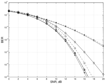
Figure 3: Average BER performance of the ZF-BDFD for the various precoders and the linear ZF detector with its optimal precoder in the scalar frequency-selective fading channel scenario in Section V-A. The solid curves denote performance achieved in the absence of error propagation, and the dashed curves incorporate the effects of error propagation. Legend—$\ast$: optimized scheme, ${\mathbf{F}}_{\text{{opt-zf-bdfd}}}$; $\circ$: direct (SCZP), ${\mathbf{F}}_{\text{{i}}}$; $\times$: DFT (ZP-OFDM), ${\mathbf{F}}_{\text{{dft}}}$; $\diamond$: optimized linear ZF scheme, ${\mathbf{F}}_{\text{{opt-zf-l}}}$.

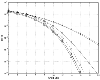
Figure 4: Average BER performance of the MMSE-BDFD for the various precoders and the linear MMSE detector with its optimal precoder in the scalar frequency-selective fading channel scenario in Section V-A. The solid curves denote performance achieved in the absence of error propagation, and the dashed curves incorporate the effects of error propagation. Legend—$\vartriangle$: optimized scheme, ${\mathbf{F}}_{\text{{opt-mmse-bdfd}}}$; $\circ$: direct (SCZP), ${\mathbf{F}}_{\text{{i}}}$; $\times$: DFT (ZP-OFDM), ${\mathbf{F}}_{\text{{dft}}}$; $\Box$: optimized linear MMSE scheme, ${\mathbf{F}}_{\text{{opt-mmse-l}}}$.

An interesting by-product of the above performance evaluation is the good performance provided by the (channel independent) direct transmission scheme (SCZP). In fact, the SCZP scheme is an optimal channel independent transmission scheme for systems that employ linear [31] or maximum likelihood [49, 55] detection, and it approaches the diversity-multiplexing trade-off for a standard class of FIR channels as the block length grows [21]. These desirable characteristics are due, in part, to the fact that the SCZP scheme preserves the good conditioning properties implicit in the tall lower-triangular Toeplitz structure of the channel matrix.

V-B Multiple antenna systems

In this example, we consider the case of narrowband transmission over a multiple antenna channel with at least as many receiver antennas as transmitter antennas. In this scenario, the combination of the direct transmission scheme and a BDFD is sometimes referred to as (uncoded) V-BLAST with a (fixed-order) “nulling and cancelling” receiver [4, 18, 20]. We consider a standard Rayleigh model for the channel in which the paths between antennas are modelled as independent zero-mean circular Gaussian random variables of unit variance.

We will focus on scenarios with $K=3$ transmitter antennas and $P=3$ or $4$ receiver antennas in which $M=K=3$ symbols are transmitted per channel use. Each element of ${\mathbf{s}}$ is an independent and equally-likely 4–QAM symbol. Therefore, the bit rate of each scheme is 6 bits-per-channel-use (bpcu). In Figs 5 and 6, we plot the average BER performance over ten thousand channel realizations of the various transmission schemes with the ZF receivers, and in Figs 7 and 8 we plot the corresponding curves for the MMSE receivers. While most of the basic trends from the case of the scalar frequency-selective channels are maintained in the multiple antenna scenario, the performance advantages of the precoders designed in Section III are much greater. (The SNR gains are of the order of 6–8 dB at a BER of $10^{-4}$.) This can be attributed to the fact that the channel matrix ${\mathbf{H}}$ does not possess any deterministic structure. In particular, the probability of encountering a channel matrix that does not have $M$ substantial singular values is not negligible. Since the proposed designs provide significantly better performance in those cases, the average performance is also substantially improved.

As expected, the performance of the optimized ZF-BDFD scheme in the absence of error propagation in Figs 5 and 6 is equal to the lower bound on $\tilde{P}_{e}$ in (38). (Recall that we are using 4-QAM signalling.) However, in the MMSE-BDFD case, the lower bound on $\tilde{P}_{e}$ in (41) is distinguishable from the simulated BER in the absence of error propagation. This is due to the fact that the block size ($M=3$) is small enough for the inaccuracy of the Gaussian approximation of the residual interference to result in a discernible difference between the BER and $\tilde{P}_{e}$. That said, even for this small block size, $\tilde{P}_{e}$ is an accurate approximation of the BER in the absence of error propagation.

A few other features of Figs 5–8 are worthy of note. First, the average performance of the direct and DFT transmission schemes are essentially the same. This is to be expected because the statistics of ${\mathbf{H}}$ are unitarily invariant. Second, the increase in the diversity provided by the channel when using $P=4$ receiver antennas rather than $P=3$ is clear from the different slopes of the BER curves at high SNR. Finally, the performance advantage of the optimized MMSE-BDFD scheme over the optimized ZF-BDFD scheme is significant in the case of $P=4$ receiver antennas and is substantial in the case of $P=3$. The performance advantage of the optimized MMSE-BDFD scheme is due, in part, to the fact the power allocated to the first $M$ eigenmodes of ${\mathbf{H}}^{H}{\mathbf{R}}_{vv}^{-1}{\mathbf{H}}$ depends on the corresponding eigenvalues. In particular, weak eigenmodes might not be allocated any power at all. In contrast, the optimized ZF-BDFD scheme allocates power uniformly over these eigenmodes. The larger performance advantage of the optimized MMSE-BDFD scheme in the case of $P=3$ is due to the larger probability of encountering a channel matrix such that ${\mathbf{H}}^{H}{\mathbf{R}}_{vv}^{-1}{\mathbf{H}}$ does not have $M=3$ significant eigenvalues.

For reference, we have included the performance of a standard orthogonal space-time block coding (OSTBC) scheme in Figs 5–8. (Like the direct and DFT transmission schemes, OSTBC schemes were designed to be applied without knowledge of the channel at the transmitter.) We have used the (symbol) rate $3/4$ code in [19] (which is a simplified version of that in [45]), and hence in order to achieve a bit rate of 6 bpcu, a natural choice for the underlying constellation is 256–QAM. (We assume that the channel is constant for the four channel uses that are required to transmit the codewords.) As expected, at high SNR, the OSTBC scheme provides better BER performance than that direct transmission (V-BLAST) scheme. However, the proposed precoder (which exploits knowledge of the channel) provides substantially better performance when $P=4$ receiver antennas are employed, and when $P=3$ and the MMSE-BDFD receiver is used.

When $P=3$ receiver antennas are employed and the ZF-BDFD is used, the OSTBC scheme performs better than the optimized scheme at high SNRs. This does not contradict the optimality of the proposed transceiver design, because the values of $M$, $K$ and $P$, and the structure of the channel matrix, are different for the OSTBC scheme. The good performance of the OSTBC scheme at high SNRs is simply a manifestation of the trade-off between error rate (achievable diversity) and symbol rate in multiple antenna fading channels without outer codes [46]. (That trade-off is related to the fundamental diversity-multiplexing trade-off [58].) The symbol rate of the OSTBC scheme is significantly lower than that of the proposed scheme. Hence, in the range of SNRs in which noise dominates the error performance, the proposed scheme provides better performance than the OSTBC scheme, but in the SNR range in which the channel condition dominates the error performance, the OSTBC scheme provides better performance. To illustrate that point, in Fig. 5 we plotted with unmarked curves the performance of the proposed ZF-BDFD scheme with a symbol rate of $M=2$ (as distinct from the scheme with $M=3$ described above). In order to maintain a bit rate of 6 bpcu, the elements of ${\mathbf{s}}$ were taken, in an independent and equally-likely fashion, from an 8–QAM constellations, and for consistency, the SNR was defined to be $(p_{0}/3)/\sigma^{2}$. Over the range of SNRs considered, the performance of the proposed ZF-BDFD scheme with $M=2$ is substantially better than that of the OSTBC scheme, with SNR gains of over 7 dB.

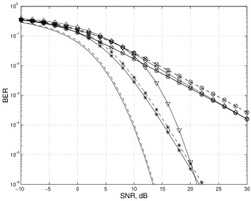
Figure 5: Average BER performance of the ZF-BDFD for the various precoders and the linear ZF detector with its optimal precoder in the narrowband multiple antenna scenario in Section V-B with $3$ transmitter antennas, $3$ receiver antennas and $M=3$ symbols per block. The solid curves denote performance achieved in the absence of error propagation, and the dashed curves incorporate the effects of error propagation. Legend—$\ast$: optimized scheme, ${\mathbf{F}}_{\text{{opt-zf-bdfd}}}$; $\circ$: direct, ${\mathbf{F}}_{\text{{i}}}$; $\times$: DFT, ${\mathbf{F}}_{\text{{dft}}}$; $\diamond$: optimized linear ZF scheme, ${\mathbf{F}}_{\text{{opt-zf-l}}}$; $\triangledown$: OSTBC. For later reference, the unmarked curves are for the optimized scheme with $M=2$.

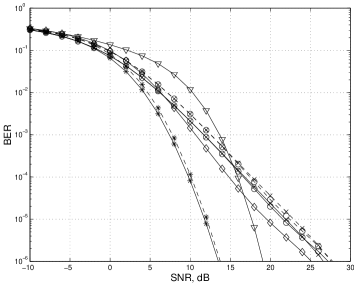
Figure 6: Average BER performance of the ZF-BDFD for the various precoders and the linear ZF detector with its optimal precoder in the narrowband multiple antenna scenario in Section V-B with 3 transmitter antennas and 4 receiver antennas. The legend is the same as that in Figure 5.

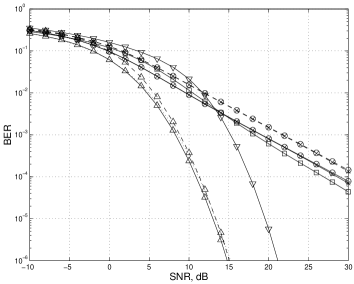
Figure 7: Average BER performance of the MMSE-BDFD for the various precoders and the linear MMSE detector with its optimal precoder in the narrowband multiple antenna scenario in Section V-B with 3 transmitter antennas and 3 receiver antennas. The solid curves denote performance achieved in the absence of error propagation, and the dashed curves incorporate the effects of error propagation. Legend—$\vartriangle$: optimized scheme, ${\mathbf{F}}_{\text{{opt-mmse-bdfd}}}$; $\circ$: direct, ${\mathbf{F}}_{\text{{i}}}$; $\times$: DFT, ${\mathbf{F}}_{\text{{dft}}}$; $\Box$: optimized linear ZF scheme, ${\mathbf{F}}_{\text{{opt-mmse-l}}}$; $\triangledown$: OSTBC. The dotted curve denotes the lower bound on $\tilde{P}_{e}$ in (41).

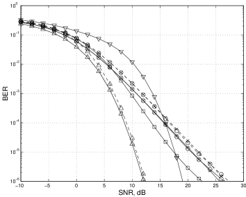
Figure 8: Average BER performance of the MMSE-BDFD for the various precoders and the linear MMSE detector with its optimal precoder in the narrowband multiple antenna scenario in Section V-B with 3 transmitter antennas, 4 receiver antennas. The legend is the same as that in Figure 7.

VI Conclusion

In this paper, we have jointly designed the precoder and the feedback matrix of a block-by-block transmission scheme equipped with a zero-forcing or minimum mean-square error (MMSE) intra-block decision feedback detector (BDFD). The designs minimize the arithmetic mean of the expected squared errors at the decision point, under the standard assumption that the previous symbols were correctly detected. The covariance matrix of the minimized error is white, and hence the proposed designs also minimize the (dominant components of the) bit error rate of a uniformly bit-loaded transmission system. In our simulations, the proposed systems performed significantly better than standard precoding systems, and retained their performance advantages in the presence of error propagation. In the case of the MMSE-BDFD, the proposed design also maximizes the Gaussian mutual information. Since the MMSE-BDFD is a “canonical” receiver [9, 10, 23], this suggests that by using the proposed transceiver design, one can approach the capacity of the block transmission system using (independent instances of) the same (Gaussian) code for each element of the block.

Appendix A Algorithm for Lemma 1

To state the algorithm succinctly, we make the following definitions: $g=\bigl{(}\prod_{k=1}^{M}\gamma_{k}^{2}\bigr{)}^{1/M}$; $[{\mathbf{S}}]_{\cdot k}$ denotes the $k$th column of ${\mathbf{S}}$ and $s_{\ell k}$ denotes its elements; ${\mathbf{Z}}_{k}$ denotes the first $k$ columns of ${\mathbf{S}}$ and ${\mathbf{Z}}_{k}^{\perp}$ denotes its orthogonal complement; $\mathcal{P}_{{\mathbf{A}}}={\mathbf{I}}-{\mathbf{A}}({\mathbf{A}}^{H}{\mathbf{A}})^{-1}{\mathbf{A}}^{H}$. The recursion will be based on the $(M-k)\times(M-k)$ matrix

$${\mathbf{A}}^{(k)}=\bigl{(}\boldsymbol{\Gamma}\mathbf{Z}_{k}^{\perp}\bigr{)}^{H}{\mathcal{P}}_{(\boldsymbol{\Gamma}\mathbf{Z}_{k}^{\perp})}\boldsymbol{\Gamma}\mathbf{Z}_{k}^{\perp}.$$ (46)

For convenience, we assume that the elements of $\boldsymbol{\Gamma}$ are arranged in non-increasing order. The algorithm proceeds as follows:

1. Initialization: Set $k=1$. An explicit solution for the first column of ${\mathbf{S}}$ is $s_{11}=\sqrt{\frac{g-\gamma_{M}^{2}}{\gamma_{1}^{2}-\gamma_{M}^{2}}}$,
   $s_{M1}=\sqrt{\frac{\gamma_{1}^{2}-g}{\gamma_{1}^{2}-\gamma_{M}^{2}}}$, $\quad s_{\ell 1}=0$ for $\ell=2,3,\cdots,M-1$.

2. Construct ${\mathbf{A}}^{(k)}$ in (46) and its eigen decomposition, ${\mathbf{A}}^{(k)}={\mathbf{V}}^{(k)}{\boldsymbol{\Lambda}}^{(k)}\bigl{(}{\mathbf{V}}^{(k)}\bigr{)}^{H}$.

3. Set the $(k+1)$th column of ${\mathbf{S}}$ to be $[{\mathbf{S}}]_{\cdot k+1}={{\mathbf{Z}}}_{k}^{\perp}{\mathbf{V}}^{(k)}{\mathbf{y}}^{(k)}$, where $y_{1}^{(k)}=\sqrt{\frac{g-\lambda^{(k)}_{M-k}}{\lambda^{(k)}_{1}-\lambda^{(k)}_{M-k}}}$,
   $y_{M-k}^{(k)}=\sqrt{\frac{\lambda^{(k)}_{1}-g}{\lambda^{(k)}_{1}-\lambda^{(k)}_{M-k}}}$, $\quad y_{\ell}^{(k)}=0$ for $\ell=2,3,\cdots,M-k-1$.

4. Increment $k$. If $k\leq M-2$ return to 2. Otherwise, set $[{\mathbf{S}}]_{\cdot M}={{\mathbf{Z}}}_{M-2}^{\perp}{\mathbf{V}}^{(M-2)}{\mathbf{y}}^{(M-1)}$, where $y_{1}^{(M-1)}=-\sqrt{\frac{g-\lambda^{(M-2)}_{2}}{\lambda^{(M-2)}_{1}-\lambda^{(M-2)}_{2}}}$, $\quad y_{2}^{(M-1)}=\sqrt{\frac{\lambda^{(M-2)}_{1}-g}{\lambda^{(M-2)}_{1}-\lambda^{(M-2)}_{2}}}$.

Appendix B Analytic Performance Comparisons

It was shown in Section IV that the precoders designed in Section III achieve the minimized value of the lower bound on $\tilde{P}_{e}$; c.f., (38) and (41). Therefore, the relative BER performance of the optimized ZF-BDFD and MMSE-BDFD systems in the absence of error propagation can be determined by simply comparing the optimal values of the MSE, $\bar{e}^{2}=\operatorname{tr}({\mathbf{R}}_{ee})/M$. (A preliminary version of this appendix appeared in [33], and related results on the MSEs of conventional decision feedback equalizers appear in [2, Chapter 8].)

In order to ensure that the ZF systems exist, we will assume that $\operatorname{rank}({\mathbf{H}})\geq M$, and to simplify the comparisons, we will also assume that the transmitted power $p_{0}$ is large enough that $q=M$ in (29) for the MMSE-BDFD and $\ell=M$ in (45) for the linear MMSE detector. Proposition 1 states that the minimum value of the MSE for a ZF-BDFD system is

$$\bar{e}_{\text{{opt-zf-bdfd}}}^{2}=\frac{M}{p_{0}}\>|\tilde{\boldsymbol{\Lambda}}_{M}|^{-1/M},$$

and Proposition 2 states that the minimum value of the MSE for an MMSE-BDFD system is

$$\bar{e}_{\text{{opt-mmse-bdfd}}}^{2}=\frac{M}{p_{0}+\operatorname{tr}(\tilde{\boldsymbol{\Lambda}}_{M}^{-1})}\>|\tilde{\boldsymbol{\Lambda}}|^{-1/M}.$$

Since $\tilde{\boldsymbol{\Lambda}}_{M}$ is positive definite, $\bar{e}_{\text{{opt-mmse-bdfd}}}^{2}<\bar{e}_{\text{{opt-zf-bdfd}}}^{2}$, and hence, in the absence of error propagation, the optimized MMSE-BDFD system will provide a lower BER than the optimized ZF-BDFD system. While it is intuitively obvious that for a given precoder, the MMSE-BDFD will provide a lower MSE than the ZF-BDFD, in the case of optimized precoders, this lower MSE leads directly to a lower BER.

The analysis of Section IV remains valid for systems with linear detectors, so long as the constraint ${\mathbf{B}}=\boldsymbol{0}$ is enforced. Therefore, we can compare the BER performance of an optimized BDFD system with that of the system that is optimized for the corresponding linear detector by simply comparing their minimum MSEs. The minimum MSE of a system with a linear ZF detector is [12]

$$\bar{e}_{\text{{opt-zf-l}}}^{2} =\frac{1}{Mp_{0}}\>\bigl{(}\operatorname{tr}(\tilde{\boldsymbol{\Lambda}}_{M}^{-1/2})\bigr{)}^{2},$$

$$\geq\frac{M}{p_{0}}\>|\tilde{\boldsymbol{\Lambda}}_{M}|^{-1/M}=\bar{e}_{\text{{opt-zf-bdfd}}}^{2},$$

where we have used the trace-determinant inequality (16). Therefore, in the absence of error propagation the optimized system for the ZF-BDFD will provide a lower BER than the optimized system for the linear ZF detector. Similarly, the minimum MSE of a system with a linear MMSE detector is [6, 36]

$$\bar{e}_{\text{{opt-mmse-l}}}^{2}$$

$$\qquad=\frac{1}{M\bigl{(}p_{0}+\operatorname{tr}(\tilde{\boldsymbol{\Lambda}}_{M}^{-1})\bigr{)}-\bigl{(}\operatorname{tr}(\tilde{\boldsymbol{\Lambda}}_{M}^{-1/2})\bigr{)}^{2}}\>\bigl{(}\operatorname{tr}(\tilde{\boldsymbol{\Lambda}}_{M}^{-1/2})\bigr{)}^{2},$$

$$\qquad>\frac{M}{p_{0}+\operatorname{tr}(\tilde{\boldsymbol{\Lambda}}_{M}^{-1})}\>|\tilde{\boldsymbol{\Lambda}}_{M}|^{-1/M}=\bar{e}_{\text{{opt-mmse-bdfd}}}^{2},$$

and hence the optimized system for the MMSE-BDFD provides a lower BER than the optimized system for the linear MMSE detector. As observed in [6], $\bar{e}_{\text{{opt-mmse-l}}}^{2}\leq\bar{e}_{\text{{opt-zf-l}}}^{2}$, and hence the optimized system for the linear MMSE detector provides a lower BER than the optimized system for the linear ZF detector.

References

- [1] S. A. Altekar and N. C. Beaulieu, “Upper Bounds on the Error Probability of Decision Feedback Equalization”, IEEE Trans. Informat. Theory, vol. 39, pp. 145–156, Jan. 1993.
- [2] J. R. Barry, E. A. Lee, and D. G. Messerschmitt, Digital Communication, 3rd edition, Kluwer, Boston, 2004.
- [3] C. A. Belfiore and J. H. Park, Jr., “Decision Feedback Equalization”, Proc. IEEE, vol. 67, pp. 1143–1156, Aug. 1979.
- [4] E. Biglieri, G. Taricco and A. Tulino, “Decoding Space-Time Codes with BLAST Architectures,” IEEE Trans. Signal Processing, vol. 50, pp. 2547–2552, Oct. 2002.
- [5] J. A. C. Bingham, “Multicarrier Modulation for Data Transmission: An Idea Whose Time Has Come”, IEEE Commun. Mag., pp. 5–14, May 1990.
- [6] S. S. Chan, T. N. Davidson and K. M. Wong, “Asymptotically Minimum BER Linear Block Precoders for MMSE Equalization”, IEE Proc.—Commun., vol. 151, pp. 297–304, Aug. 2004.
- [7] K. Cho and D. Yoon, “On the general BER expression of one and two dimensional amplitude modulations,” IEEE Trans. Commun., vol. 50, pp. 1074–1080, July 2002.
- [8] J. S. Chow, J. C. Tu and J. M. Cioffi, “Performance Evaluation of a Multichannel Transceiver System for ADSL and VHDSL Receivers”, IEEE J. Select. Areas Commun., vol. 9, pp. 909–919, Aug. 1991.
- [9] J. M. Cioffi, G. P. Dudevoir, M. V. Eyuboglu and G. D. Forney, “MMSE Decision-Feedback Equalizers and Coding—Part I: Equalization Results; Part II: Coding Results”, IEEE Trans. Commun., vol. 43, pp. 2582–2604, Oct. 1995.
- [10] J. M. Cioffi and G. D. Forney, “Generalized Decision-Feedback Equalization for Packet Transmission with ISI and Gaussian Noise”, in Communications, Computation, Control and Signal Processing, A. Paulraj, V. Roychowdhury and C. Schaper, Eds, Kluwer, Boston, 1997.
- [11] T. M. Cover and J. A. Thomas, Elements of Information Theory. Wiley, New York, 1991.
- [12] Y. W. Ding, T. N. Davidson, Z.-Q. Luo, and K. M. Wong, “Minimum BER Block Precoders for Zero-Forcing Equalization”, IEEE Trans. Signal Processing, vol. 51, pp. 2410–2423, Sept. 2003.
- [13] Y. W. Ding, T. N. Davidson, and K. M. Wong, “On Improving the BER Performance of Rate-Adaptive Block Transceivers, with Applications to DMT”, in Proc. IEEE Global Commun. Conf., San Francisco, CA, Dec. 2003.
- [14] A. Duel-Hallen, “Decorrelating Decision-Feedback Multiuser Detector for Synchronous Code-Division Multiple-Access Channels”, IEEE Trans. Commun., vol. 41, pp. 285–290, Feb. 1993.
- [15] A. Duel-Hallen, “A Family of Multiuser Decision-Feedback Detectors for Asynchronous Code-Division Multiple-Access Channels”, IEEE Trans. Commun., vol. 43, pp. 421–434, Feb./Mar./Apr. 1995.
- [16] D. L. Duttweiler, J. E. Mazo, and D. G. Messerschmitt, “An Upper Bound on the Error Probability in Decision-Feedback Equalization”, IEEE Trans. Informat. Theory, vol. IT–20, pp. 490–497, July 1974.
- [17] D. Falconer and G. Foschini, “Theory of Minimum Mean-Square-Error QAM Systems Employing Decision Feedback Equalization”, Bell Syst. Tech. J., vol. 52, pp. 1821–1849, Dec. 1973.
- [18] G. J. Foschini, G. D. Golden, R. A. Valenzuela and P. W. Wolniansky, “Simplified Processing for High Spectral Efficiency Wireless Communication Employing Multi-Element Arrays”, IEEE J. Select. Areas Commun., vol. 17, pp. 1841–1852, Nov. 1999.
- [19] G. Ganesan and P. Stoica, “Space-Time Block Coses: A Maximum SNR Approach,” IEEE Trans. Informat. Theory, vol. 47, pp. 1650–1656, May 2001.
- [20] G. Ginis and J. M. Cioffi, “On the Relation Between V-BLAST and GDFE”, IEEE Commun. Lett., vol. 5, pp. 364–366, Sep. 2001.
- [21] L. Grokop and D. N. C. Tse, “Diversity/Multiplexing Tradeoff in ISI Channels,” in Proc. Int. Symp. Informat. Theory, Chicago, June 2004. p. 97.
- [22] T. Guess, “Optimal Sequences for CDMA with Decision-Feedback Receivers”, IEEE Trans. Informat. Theory, vol. 49, pp. 886–900, Apr. 2003.
- [23] T. Guess and M. K. Varanasi, “An Information Theoretic Framework for Deriving Canonical Decision-Feedback Receivers in Gaussian Channels”, IEEE Trans. Informat. Theory, vol. 51, pp. 173–187, Jan. 2005.
- [24] T. Guess and M. K. Varanasi, “A New Successively Decodable Coding Technique for Intersymbol-Interference Channels”, in Proc. Int. Symp. Informat. Theory, Sorrento, Italy, June 2000.
- [25] D. Guo, S. Verdù and L. K. Rasmussen, “Asymptotic Normality of Linear Multiuser Receiver Outputs,” IEEE Trans. Informat. Theory, vol. 48, pp. 3080–3095, Dec. 2002.
- [26] B. Hassibi and B. M. Hochwald, “High-Rate Codes that are Linear in Space and Time,” IEEE Trans. Informat. Theory, vol. 48, pp. 1804–1824, July 2002.
- [27] R. A. Horn and C. R. Johnson, Matrix Analysis, Cambridge University Press, Cambridge, UK, 1985.
- [28] G. K. Kaleh, “Channel Equalization for Block Transmission System”, IEEE J. Select. Areas Commun., vol. 13, pp. 110–121, Jan. 1995.
- [29] S. Kasturia, J. T. Aslanis, and J. M. Cioffi, “Vector Coding for Partial Response Channels”, IEEE Trans. Informat. Theory, vol. 36, pp. 741–762, July 1990.
- [30] J. W. Lechleider, “The Optimum Combination of Block Codes and Receivers for Arbitrary Channels”, IEEE Trans. Commun., vol. 38, pp. 615–621, May 1990.
- [31] Y. Lin and S. M. Phoong, “BER minimized OFDM Systems with Channel Independent Precoders”, IEEE Trans. Signal Processing, vol. 51, pp. 2369–2380, Sep. 2003.
- [32] J. R. Magnus and H. Neudecker, Matrix Differential Calculus with Applications in Statistics and Econometrics, Wiley, New York, 1988.
- [33] Q. Meng, J.-K. Zhang and K. M. Wong, “Block Data Transmission: A Comparison of Performance for the MBER Precoder Designs”. in Proc. IEEE Sensor Array & Multichannel Signal Processing Wkshp, Barcelona, July 2004.
- [34] B. Muquet, Z. Wang, G. B. Giannakis, M. de Courville and P. Duhamel, “Cyclic Prefixing or Zero Padding for Wireless Multicarrier Transmissions?”, IEEE Trans. Commun., vol. 50, pp. 2136–2148, Dec. 2002.
- [35] F. D. Neeser and J. L. Massey, “Proper Complex Random Processes with Applications to Information Theory”, IEEE Trans. Informat. Theory, vol. 39, pp. 1293–1302, July 1993.
- [36] D. P. Palomar, J. M. Cioffi, and M. A. Lagunas, “Joint Tx-Rx Beamforming Design for Multicarrier MIMO Channels: A Unified Framework for Convex Optimization”, IEEE Transactions on Signal Processing, vol. 51, pp. 2381–2401, Sept. 2003.
- [37] B. Picinbono, “On Circularity,” IEEE Trans. Signal Processing, vol. 42, pp. 3474–3482, Dec. 1994.
- [38] H. V. Poor and S. Verdù, “Probability of Error in MMSE Multiuser Detection”, IEEE Trans. Informat. Theory, vol. 43, pp. 858–871, May 1997.
- [39] J. G. Proakis, Digital Communications, 4th edition, McGraw Hill, New York, 2001.
- [40] J. Salz, “Optimum Mean-Square Decision Feedback Equalization”, Bell Syst. Tech. J., vol. 52, pp. 1341–1373, Oct. 1973.
- [41] A. Scaglione, S. Barbarossa, and G. B. Giannakis, “Filterbank Transceivers Optimizing Information Rate in Block Transmissions over Dispersive Channels”, IEEE Trans. Informat. Theory, vol. 45, pp. 1019–1032, Apr. 1999.
- [42] A. Scaglione, G. B. Giannakis and S. Barbarossa, “Redundant Filterbank Precoders and Equalizers Part I: Unification and Optimal Designs”, IEEE Trans. Signal Processing, vol. 47, pp. 1988–2005, July 1999.
- [43] A. Scaglione, P. Stoica, S. Barbarossa, G. B. Giannakis, and H. Sampath, “Optimal Designs for Space-Time Linear Precoders and Decoders”, IEEE Trans. Signal Processing, vol. 50, pp. 1051–1064, May 2002.
- [44] A. Stamoulis, G. B. Giannakis, and A. Scaglione, “Block FIR Decision-Feedback Equalizers for Filterbank Precoded Transmissions with Blind Channel Estimation Capabilities,” IEEE Trans. Commun., vol. 49, pp. 69–83, Jan. 2001.
- [45] V. Tarokh, H. Jafarkhani and A. R. Calderbank, “Space-Time Block Codes from Orthogonal Designs,” IEEE Trans. Informat. Theory, vol. 45, pp. 1456–1467, July 1999.
- [46] B. Varadarajan and J. R. Barry, “The Rate-Diversity Trade-off for Linear Space-Time Codes,” in Proc. IEEE Veh. Tech. Conf., Vancouver, Sep. 2002, vol. 1, pp. 67–71.
- [47] M. K. Varanasi, “Decision Feedback Multiuser Detection: A Systematic Approach”, IEEE Trans. Informat. Theory, vol. 45, pp. 110–121, Jan. 1999.
- [48] M. K. Varanasi and T. Guess, “Optimum Decision Feedback Multiuser Equalization with Successive Decoding Achieves the Total Capacity of the Gaussian Multiple-Access Channel”, in Proc. Asilomar Conf. Signals, Systems, Computers, Monteray, CA, Nov. 1997.
- [49] Z. Wang, X. Ma, and G. B. Giannakis, “OFDM or Single-Carrier Block Transmissions?”, IEEE Trans. Commun., vol. 52, pp. 380–394, Mar. 2004.
- [50] H. S. Witsenhausen, “A Determinant Maximization Problem Occurring in the Theory of Data Communication”, SIAM J. Appl. Math., vol. 29, pp. 515–522, Nov. 1975.
- [51] F. Xu, T. N. Davidson, and K. M. Wong, “Design of Block-by-Block Transceivers with Successive Detection”, in Proc. IEEE SP Wkshp Signal Processing Adv. Wireless Commun., Rome, Italy, June 2003.
- [52] J. Yang and S. Roy, “Joint Transmitter-Receiver Optimization for Multi-Input Multi-Output Systems with Decision Feedback”, IEEE Trans. Informat. Theory, vol. 40, pp. 1334–1347, Sep. 1994.
- [53] D. Yoon and K. Cho, “General Bit Error Probability of Rectangular Quadrature Amplitude Modulation,” Electronics Lett., vol. 38, pp. 131–133, Jan. 2002.
- [54] J. Zhang, E. K. P. Chong and D. N. C. Tse, “Output MAI Distributions of Linear MMSE Multiuser Receivers in DS-CDMA Systems”, IEEE Trans. Informat. Theory, vol. 47, pp. 1128–1144, Mar. 2001.
- [55] J.-K. Zhang, T. N. Davidson, and K. M. Wong, “Optimal Precoder for Block Transmission over Frequency-Selective Fading Channels” To appear in the IEE Proc.—Commun.
- [56] J.-K. Zhang, A. Kavčić, X. Ma, and K. M. Wong, “Design of Unitary Precoders for ISI Channels”, in Proc. Int. Conf. Acoust., Speech, and Signal Processing, Orlando, FL, Apr. 2002, pp. 2265–2268.
- [57] J.-K. Zhang, A. Kavčić, and K. M. Wong, “Equal Diagonal QR Decomposition and its Application to Precoder Design for Successive-Cancellation Detection”, IEEE Trans. Informat. Theory, vol. 51, pp. 154–172, Jan. 2005.
- [58] L. Zheng and D. N. C. Tse, “Diversity and Multiplexing: A Fundamental Tradeoff in Multiple-Antenna Channels,” IEEE Trans. Informat. Theory, vol. 49, pp. 1073–1096, May 2003.