Network Information Flow
with Correlated Sources

Abstract

Consider the following network communication setup, originating in a sensor networking application we refer to as the “sensor reachback” problem. We have a directed graph $G=(V,E)$, where $V=\{v_{0}v_{1}...v_{n}\}$ and $E\subseteq V\times V$. If $(v_{i},v_{j})\in E$, then node $i$ can send messages to node $j$ over a discrete memoryless channel $(\mathcal{X}_{ij},p_{ij}(y|x),\mathcal{Y}_{ij})$, of capacity $C_{ij}$. The channels are independent. Each node $v_{i}$ gets to observe a source of information $U_{i}$ ($i=0...M$), with joint distribution $p(U_{0}U_{1}...U_{M})$. Our goal is to solve an incast problem in $G$: nodes exchange messages with their neighbors, and after a finite number of communication rounds, one of the $M+1$ nodes ($v_{0}$ by convention) must have received enough information to reproduce the entire field of observations $(U_{0}U_{1}...U_{M})$, with arbitrarily small probability of error. In this paper, we prove that such perfect reconstruction is possible if and only if

$$H(U_{S}|U_{S^{c}})\;\;<\;\;\sum_{i\in S,j\in S^{c}}C_{ij},$$

for all $S\subseteq\{0...M\}$, $S\neq\emptyset$, $0\in S^{c}$. Our main finding is that in this setup a general source/channel separation theorem holds, and that Shannon information behaves as a classical network flow, identical in nature to the flow of water in pipes. At first glance, it might seem surprising that separation holds in a fairly general network situation like the one we study. A closer look, however, reveals that the reason for this is that our model allows only for independent point-to-point channels between pairs of nodes, and not multiple-access and/or broadcast channels, for which separation is well known not to hold [5, pp. 448-49]. This “information as flow” view provides an algorithmic interpretation for our results, among which perhaps the most important one is the optimality of implementing codes using a layered protocol stack.

I Introduction

I-A The Sensor Reachback Problem

Wireless sensor networks made up of small, cheap, and mostly unreliable devices equipped with limited sensing, processing and transmission capabilities, have recently sparked a fair amount of interest in communications problems involving multiple correlated sources and large-scale wireless networks [6]. It is envisioned that an important class of applications for such networks involves a dense deployment of a large number of sensors over a fixed area, in which a physical process unfolds—the task of these sensors is then to collect measurements, encode them, and relay them to some data collection point where this data is to be analyzed, and possibly acted upon. This scenario is illustrated in Fig. 1.

Figure 1: A large number of sensors is deployed over a target area. After collecting the data of interest, the sensors must reach back and transmit this information to a single receiver (e.g., an overflying plane) for further processing.

There are several aspects that make this communications problem interesting:

• Correlated Observations: If we have a large number of nodes sensing a physical process within a confined area, it is reasonable to assume that their measurements are correlated. This correlation may be exploited for efficient encoding/decoding.

• Cooperation among Nodes: Before transmitting data to the remote receiver, the sensor nodes may establish a conference to exchange information over the wireless medium and increase their efficiency or flexibility through cooperation.

• Channel Interference: If multiple sensor nodes use the wireless medium at the same time (either for conferencing or reachback), their signals will necessarily interfere with each other. Consequently, reliable communication in a reachback network requires a set of rules that control (or exploit) the interference in the wireless medium.

In order to capture some of these key aspects, while still being able to provide complete results, we make some modeling assumptions, discussed next.

I-A1 Source Model

We assume that the sources are memoryless, and thus consider only the spatial correlation of the observed samples and not their temporal dependence (since the latter dependencies could be dealt with by simple extensions of our results to the case of ergodic sources). Furthermore, each sensor node $v_{i}$ observes only one component $U_{i}$ and must transmit enough information to enable the sink node $v_{0}$ to reconstruct the whole vector $U_{1}U_{2}\dots U_{M}$. This assumption is the most natural one to make for scenarios in which data is required at a remote location for fusion and further processing, but the data capture process is distributed, with sensors able to gather local measurements only, and deeply embedded in the environment.

A conceptually different approach would be to assume that all sensor nodes get to observe independently corrupted noisy versions of one and the same source of information $U$, and it is this source (and not the noisy measurements) that needs to be estimated at a remote location. This approach seems better suited for applications involving non-homogeneous sensors, where each one of the sensors gets to observe different characteristics of the same source (e.g., multispectral imaging), and therefore leads to a conceptually very different type of sensing applications from those of interest in this work. Such an approach leads to the so called CEO problem studied by Berger, Zhang and Viswanathan in [7].

I-A2 Independent Channels

Our motivation to consider a network of independent DMCs is twofold.

From a pure information-theoretic point of view independent channels are interesting because, as shown in this paper, this assumption gives rise to long Markov chains which play a central role in our ability to prove the converse part of our coding theorem, and thus obtain conclusive results in terms of capacity. Moreover, a corollary of said coding theorem does provide a conclusive answer for a special case of the multiple access channel with correlated sources, a problem for which no general converse is known.

From a more practical point of view, the assumption of independent channels is valid for any network that controls interference by means of a reservation-based medium-access control protocol (e.g., TDMA). This option seems perfectly reasonable for sensor networking scenarios in which sensors collect data over extended periods of time, and must then transmit their accumulated measurements simultaneously. In this case, a key assumption in the design of standard random access techniques for multiaccess communication breaks down—the fact that individual nodes will transmit with low probability [8, Chapter 4]. As a result, classical random access would result in too many collisions and hence low throughput. Alternatively, instead of mitigating interference, a medium access control (MAC) protocol could attempt to exploit it, in the form of using cooperation among nodes to generate waveforms that add up constructively at the receiver (cf. [9, 10, 11]). Providing an information-theoretic analysis of such cooperation mechanisms would be very desirable, but since it entails dealing with correlated sources and a general multiple access channel, dealing with correlated sources and an array of independent channels constitutes a reasonable first step towards that goal, and is also interesting in its own right, since it provides the ultimate performance limits for an important class of sensor networking problems.

I-A3 Perfect Reconstruction at the Receiver

In our formulation of the sensor reachback problem, the far receiver is interested in reconstructing the entire field of sensor measurements with arbitrarily small probability of error. This formulation leads us to a natural capacity problem, in the classical sense of Shannon. Alternatively, one could relax the condition of perfect reconstruction, and tolerate some distortion in the reconstruction of the field of measurements at the far receiver, thus leading to the so called Multiterminal Source Coding problem studied by Berger [12]. This condition could be further relaxed, to require a faithful reproduction of the image of some function $f$ of the sources, leading to a problem studied extensively by Csiszar, Körner and Marton [13, 14].

I-B An Information Theoretic View of Architectural Issues

For large-scale, complex systems of the type of interest in this work, the complexity of basic questions of design and performance analysis appears daunting:

• How should nodes cooperate to relay messages to the data collector node $v_{0}$? Should they decode received messages, re-encode them, and forward to other nodes? Should they map channel outputs to channel inputs without attempting to decode? Should they do something else?

• How should redundancy among the sources be exploited? Should we compress the information as much as possible? Should we leave some of that redundancy to combat noise in the channels? Is there a source/channel separation theorem in these networks?

• How do we measure performance of these networks, what are appropriate cost metrics? How do we design networks that are efficient under an appropriate cost metric?

In [15], a number of examples are identified in which the existence of a simple architecture has played an enabling role in the proliferation of technology: the von Neuman computer architecture, separation of source and channel coding in communications, separation of plant and controller in control systems, and the OSI layered architecture model. So what all these questions boil down to is an issue similar to those considered in [15]: what are appropriate abstractions of the network, similar to the IP protocol stack for the Internet, based on which we can break the design task into independent reusable components, optimize the design of these components, and obtain an efficient system as a result? In this work, we show how information theory is indeed capable of providing very meaningful answers to this problem.

Information theory, in one of its applications, deals with the analysis of performance of communication systems. So, to some it may seem the natural theory to turn to for guidance in the task of searching for a suitable network architecture. However, to others it may seem unnatural to do so: it is well known that information theory and communication networks have not had fruitful interactions in the past, as explained by Ephremides and Hajek [16]. Thus, in the presence of these mixed indicators, we take the stand that indeed information theory has a great deal to offer in the task at hand. And to justify our position, consider Shannon’s model for a communications system, as illustrated in Fig. 2.

Figure 2: Shannon’s model for a point-to-point system. Top figure: abstract view, consisting of a source, an encoder from source symbols to channel symbols, a conditional probability distribution to model the random dependence of outputs on inputs, and a decoder to map from received messages back to source symbols; bottom figure: a capacity-achieving architecture for this system, in which error control codes are used to create an illusion of a noiseless bit pipe.

For this setup, Shannon established that reliable communication of a source over a noisy channel is possible if and only if the entropy rate of the source is less than the capacity of the channel [5, Ch. 8.13]. This result, known as the source/channel separation theorem, has a double significance. On one hand, it provides an exact single-letter characterization of conditions under which reliable communication is possible. On the other hand, and of particular interest to the task at hand for us, it is a statement about the architecture of an optimal communication system: the encoder/decoder design task can be split into the design and optimization of two independent components. So it is inspired by Shannon’s teachings for point-to-point systems that we ask in this work, and answer in the affirmative, the question of whether it is possible or not to derive similar useful architectural guidelines for the class of networks under consideration.

I-C Related Work

The problem of communicating distributed correlated sources over a network of point-to-point links is closely related to several classical problems in network information theory. To set the stage for the main contributions of this paper, we now review related previous work.

I-C1 Distributed Correlated Sources and Multiple Access

The concept of separate encoding of correlated sources was studied by Slepian and Wolf in their seminal paper [17], where they proved that two correlated sources $(U_{1}U_{2})$ drawn i.i.d. $\sim p(u_{1}u_{2})$ can be compressed at rates $(R_{1},R_{2})$ if and only if

$$R_{1} \geq H(U_{1}|U_{2})$$

$$R_{2} \geq H(U_{2}|U_{1})$$

$$R_{1}+R_{2} \geq H(U_{1}U_{2}).$$

Assume now that $(U_{1}U_{2})$ are to be transmitted with arbitrarily small probability of error to a joint receiver over a multiple access channel with transition probability $p(y|x_{1}x_{2})$. Knowing that the capacity of the multiple access channel with independent sources is given by the convex hull of the set of points $(R_{1},R_{2})$ satisfying [5, Ch. 14.3]

$$R_{1} < I(X_{1};Y|X_{2})$$

$$R_{2} < I(X_{2};Y|X_{1})$$

$$R_{1}+R_{2} < I(X_{1}X_{2};Y),$$

it is not difficult to prove that Slepian-Wolf source coding of $(U_{1}U_{2})$ followed by separate channel coding yields the following sufficient conditions for reliable communication

$$H(U_{1}|U_{2}) < I(X_{1};Y|X_{2})$$

$$H(U_{2}|U_{1}) < I(X_{2};Y|X_{1})$$

$$H(U_{1}U_{2}) < I(X_{1}X_{2};Y).$$

These conditions, which basically state that the Slepian-Wolf region and the capacity region of the multiple access channel have a non-empty intersection, are sufficient but not necessary for reliable communication, as shown by Cover, El Gamal, and Salehi with a simple counterexample in [18]. In that same paper, the authors introduce a class of correlated joint source/channel codes, which enables them to increase the region of achievable rates to

$$H(U_{1}|U_{2}) < I(X_{1};Y|X_{2}U_{2})$$ (1)

$$H(U_{2}|U_{1}) < I(X_{2};Y|X_{1}U_{1})$$ (2)

$$H(U_{1}U_{2}) < I(X_{1}X_{2};Y),$$ (3)

for some $p(u_{1}u_{2}x_{1}x_{2}y)=p(u_{1}u_{2})\cdot p(x_{1}|u_{1})\cdot p(x_{2}|u_{2})\cdot p(y|x_{1}x_{2})$. Also in [18], the authors generalize this set of sufficient conditions to sources $(U_{1}U_{2})$ with a common part $W=f(U_{1})=g(U_{2})$, but they were not able to prove a converse, i.e., they were not able to show that their region is indeed the capacity region of the multiple access channel with correlated sources. Later, it was shown with a carefully constructed example by Dueck in [19] that indeed the region defined by eqns. (1)-(3) is not tight. Related problems were considered by Slepian and Wolf [20], and Ahlswede and Han [21]. To this date however, the general problem still remains open.

Assuming independent sources, Willems investigated a cooperative scenario, in which encoders exchange messages over conference links of limited capacity prior to transmission over the multiple access channel [22]. In this case, the capacity region is given by

$$R_{1} < I(X_{1};Y|X_{2}Z)+C_{12}$$

$$R_{2} < I(X_{2};Y|X_{1}Z)+C_{21}$$

$$R_{1}+R_{2} < \min\{\;I(X_{1}X_{2};Y|Z)+C_{12}+C_{21},\;I(X_{1}X_{2};Y)\;\},$$

for some auxiliary random variable $Z$ such that $|\mathcal{Z}|\leq\min(|\mathcal{X}_{1}|\cdot|\mathcal{X}_{2}|+2,|\mathcal{Y}|+3)$, and for a joint distribution $p(zx_{1}x_{2}y_{1}y_{2})=p(z)\cdot p(x_{1}|z)\cdot p(x_{2}|z)\cdot p(y|x_{1}x_{2})$.

I-C2 Correlated Sources and Networks of DMCs

Very recently, an early paper was brought to our attention, in which Han considers the transmission of correlated sources to a common sink over a network of independent channels [23]. Although the problem setup is less general than ours, in that (a) each source block and each transmitted codeword partipate only once in the encoding process, and (b) the intermediate nodes are assumed to decode the data before passing it on, Theorem 3.1 of [23] is very similar to our Theorem 4.

Our work, done independently of Han’s, differs from it and complements it in the following ways:

• Our setup is more general. We allow for arbitrary forms of joint source-channel coding to take place inside the network while data flows towards the decoder, and then prove that a one-step encoding process, pure routing, and separate source/channel coding are sufficient. Han assumes decode-and-forward in his problem statement, as well as a one-step encoding process.

• The proof techniques are different. Han takes a purely combinatorial approach to the problem: he thoroughly exploits the polymatroidal structure of the capacity function for the network of channels, and the co-polymatroidal structure for the Slepian-Wolf region. We establish our achievability result by explicitly constructing a routing algorithm for the Slepian-Wolf indices, and our converse by standard methods based on Fano’s inequality.

Furthermore our work, being motivated by a concrete sensor networking application, establishes connections and relevance to practical engineering problems (see Section III) that are not a concern in [23].

I-C3 Network Coding

Another closely related problem is the well known network coding problem, introduced by Ahlswede, Cai, Li and Yeung [24]. In that work, the authors establish the need for applying coding operations at intermediate nodes to achieve the max-flow/min-cut bound of a general multicast network. A converse proof for this problem was provided by Borade [25]. Linear codes were proposed by Li, Yeung and Cai in [26], and Koetter and Médard in [27].

Effros, Médard et al. have developed a comprehensive study on separate and joint design of linear source, channel and network codes for networks with correlated sources under the assumption that all operations are defined over a common finite field [28]. For this particular case, optimality of separate linear source and channel coding was observed in the one-receiver instance, but the result of [28] does not prove that it holds for general networks and channels with arbitrary input and output alphabets. Error exponents for multicasting of correlated sources over a network of noiseless channels were given by Ho, Médard et al. in [29], and networks with undirected links were considered by Li and Li in [30].

Another problem in which network flow techniques have been found useful is that of finding the maximum stable throughput in certain networks. In this problem, posed by Gupta and Kumar in [31], it is sought to determine the maximum rate at which nodes can inject bits into a network, while keeping the system stable. This problem was reformulated by Peraki and Servetto as a multicommodity flow problem, for which tight bounds were obtained using elementary counting techniques [32, 33].

I-D Main Contributions and Organization of the Paper

Our main original contributions can be summarized as follows:

• A general coding theorem yielding necessary and sufficient conditions for reliable communication of $M+1$ correlated sources to a common sink over a network of independent DMCs.

• An achievability proof which combines classical coding arguments with network flow methods and a converse proof that establishes the optimality of separate source and channel coding.

• A detailed discussion on the engineering implications of our main result, and the concepts of information-theoretically optimal network architectures and protocol stacks.

The rest of the paper is organized as follows. In Section II we give formal definitions, to then state and prove our main theorem. We also look at three special cases: a network with three nodes, the non-cooperative case, and an array of orthogonal Gaussian channels. In Section III we address the practical implications of our main result, by describing an information-theoretically optimal protocol stack, elaborating on the tractability of related network architecture and network optimization problems, and discussing the suboptimality of correlated codes for orthogonal channels. The paper concludes with Section IV.

II A Coding Theorem for Network Information Flow with Correlated Sources

II-A Formal Definitions and Statement of the Main Theorem

A network is modeled as the complete graph on $M+1$ nodes. For each $(v_{i},v_{j})\in E$ ($0\leq i,j\leq M$), there is a discrete memoryless channel $(\mathcal{X}_{ij},p_{ij}(y|x),\mathcal{Y}_{ij})$, with capacity $C_{ij}=\max_{p_{ij}(x)}I(X_{ij};Y_{ij})$. At each node $v_{i}\in V$, a random variable $U_{i}$ is observed ($i=0...M$), drawn i.i.d. from a known joint distribution $p(U_{0}U_{1}...U_{M})$. Node $v_{0}$ is the decoder – the goal in this problem is to find conditions under which $U_{1}...U_{M}$ can be reproduced reliably at $v_{0}$. We now make this statement more precise, by describing how the nodes communicate and by giving the formal definitions of code, probability of error and reliable communication.

Time is discrete. Every $N$ time steps, node $v_{i}$ collects a block $U_{i}^{N}$ of source symbols – we refer to the collection of all blocks $[U_{0}^{N}(k)U_{1}^{N}(k)...U_{M}^{N}(k)]$ collected at time $kN$ ($k\geq 1$) as a block of snapshots. Node $v_{i}$ then sends a codeword ${X}_{ij}^{N}$ to node $v_{j}$. This codeword depends on a window of $K$ previous blocks of source sequences $U_{i}^{N}$ observed at node $v_{i}$, and of $T$ previously received blocks of channel outputs, corresponding to noisy versions of the codewords sent by all nodes to node $v_{i}$ in the previous $T$ communications steps (corresponding to $NT$ time steps).

For a block of snapshots observed at time $kN$, at time $(k+W)N$ (that is, after allowing for a finite but otherwise arbitrary amount of time to elapse, in which the information injected by all nodes reaches $v_{0}$), an attempt is made to decode at $v_{0}$. The decoder produces an estimate of the block of snapshots $U_{0}^{N}(k)U_{1}^{N}(k)...U_{M}^{N}(k)$ based on the local observations $U_{0}^{N}(k)$, and the previous $W$ blocks of $N$ channel outputs generated by codewords sent to $v_{0}$ by the other nodes.

Thus, a code for this network consists of:

• four integers $N$, $K$, $T$ and $W$;

• encoding functions at each node

  $$g_{ij}:\bigotimes_{l=1}^{K}\mathcal{U}_{i}^{N}\times\bigotimes_{t=1}^{T}\bigotimes_{m=0}^{M}\mathcal{Y}_{mi}^{N}\longrightarrow\mathcal{X}_{ij}^{N},$$

  for $0\leq i,j\leq M$.

• the decoding function at node $v_{0}$:

  $$h:\mathcal{U}_{0}^{N}\times\bigotimes_{w=1}^{W}\bigotimes_{m=1}^{M}\mathcal{Y}_{m0}^{N}\longrightarrow\bigotimes_{m=1}^{M}\hat{\mathcal{U}}_{m}^{N}.$$

• the block probability of error:

  $$P_{e}^{(N)}=P(U_{1}^{N}...U_{M}^{N}\neq\hat{U}_{1}^{N}...\hat{U}_{M}^{N}).$$

We say that blocks of snapshots $U_{1}^{N}...U_{M}^{N}$ can be reliably communicated to $v_{0}$ if there exists a sequence of codes as above, with $P_{e}^{(N)}\to 0$ as $N\to\infty$, for some finite values $K$, $T$ and $W$, all independent of $N$.

With these definitions, we are now ready to state our main theorem.

Theorem 1

Let $S$ denote a non-empty subset of node indices that does not contain node $0$: $S\subseteq\{0...M\}$, $S\neq\emptyset$, $0\in S^{c}$. Then, it is possible to communicate $U_{1}...U_{M}$ reliably to $v_{0}$ if and only if, for all $S$ as above,

$$H(U_{S}|U_{S^{c}})\;\;<\;\;\sum_{i\in S,j\in S^{c}}C_{ij}.$$ (4)

II-B Achievability Proof

Our coding strategy is based on separate source and channel coding. We first use capacity attaining channel codes to turn the noisy network into a network of noiseless links (of capacity $C_{ij}$). Then, we use Slepian-Wolf source codes, jointly with a custom designed routing algorithm, to deliver all this data to destination. Since the channel coding aspects of the proof are rather straightforward extensions of classical point-to-point arguments, in the following we only focus on the less obvious source coding and routing aspects.

II-B1 Mechanics of the Coding Strategy

Consider a “noise-free” version of the problem formulated above: we still have a complete graph, now with noiseless links of capacity $C_{ij}$. Variables $U_{i}$ are still observed at each node $v_{i}$, and the goal remains to reproduce all of these at $v_{0}$. Each node uses a classical Slepian-Wolf code: there is a source encoder at node $v_{i}$ that maps a sequence $U_{i}^{N}$ to an index from the random binning set $\{1,2,\dots,2^{NR_{i}}\}$, thus compressing the block of observations $U_{i}^{N}$ using codes as in [5, Thm. 14.4.2]. Let $(R_{1}...R_{M})$ denote the rate allocation to each of the nodes. To achieve perfect reconstruction, these bits must be delivered to node $v_{0}$.

• Set $K=T=1$ – each block of source symbols and each block of codewords participates in the encoding process only once.

• To deliver the bin indices produced by the Slepian-Wolf codes to destination, the noise-free network is regarded as a flow network [34, Ch. 26]. Let $\varphi(v_{i},v_{j})$ be a feasible flow in this network, with $M$ sources $v_{1}...v_{M}$, supply $R_{i}$ at source $v_{i}$, and a single sink $v_{0}$. If no such feasible flow exists, the code construction fails.

• If there is a feasible flow $\varphi$ then this $\varphi$ uniquely determines, at each node $v_{i}$, the number of bits that need to be sent to each of its neighbors – thus from $\varphi$ we derive the encoding functions $g_{ij}$ as follows:

  • Consider the directed acyclic graph $G^{\prime}$ of $G$ induced by $\varphi$, by taking $V(G^{\prime})=V(G)$, and $E(G^{\prime})=\{(v_{i},v_{j})\in E:\varphi(v_{i},v_{j})>0\}$. Define a permutation $\pi:\{0...M\}\to\{0...M\}$, such that $[v_{\pi(0)}v_{\pi(1)}...v_{\pi(M)}]$ is a topological sort of the nodes in $G$, as illustrated in Fig. 3.

    

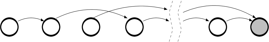
    Figure 3: A topological sort of the nodes of a directed acyclic graph is a linear ordering $v_{1}...v_{M}$ such that if $(v_{i},v_{j})$ is an edge, then $i<j$.

  • Consider a block of snapshots ${\mathbf{U}}(k)=[U_{0}^{N}(k)U_{1}^{N}(k)...U_{M}^{N}(k)]$ captured at time $kN$. At time $(k+l)N$ (for $l=0...M$), node $v_{\pi(l)}$ will have received all bits with portions of the encodings of ${\mathbf{U}}(k)$ generated by nodes upstream in the topological order – thus, together with its own encoding of $U^{N}_{\pi(l)}(k)$, all the bits for ${\mathbf{U}}(k)$ up to and including node $v_{\pi(l)}$ will be available there, and thus can be routed to nodes downstream in the topological order.

  • Consider now all edges of the form $(v_{\pi(k)},v^{\prime})$ for which $\varphi(v_{\pi(k)},v^{\prime})>0$:

    1. Collect the $m=\sum_{v^{\prime}}\varphi(v^{\prime},v_{\pi(k)})$ information bits sent by the upstream nodes $v^{\prime}$.

    2. Consider now the set of all downstream nodes $v^{\prime\prime}$, for which $\varphi(v_{\pi(k)},v^{\prime\prime})>0$. Due to flow conservation for $\varphi$, $\sum_{v^{\prime\prime}}\varphi(v_{\pi(k)},v^{\prime\prime})=m+R_{\pi(k)}$, where $R_{\pi(k)}$ is the rate allocated to node $v_{\pi(k)}$.

    3. For each $v^{\prime\prime}$ as above, define $g_{\pi(k)v^{\prime\prime}}^{(k)}$ to be a message such that $|g_{\pi(k)v^{\prime\prime}}^{(k)}|=\varphi(v_{\pi(k)},v^{\prime})$. Partition the $m+R_{\pi(k)}$ available bits according to the values of $\varphi$, and send them downstream, as illustrated in Fig. 4.

       

       Figure 4: To illustrate the operations performed at each node. In this example, five bits come into node $v_{\pi(k)}$ from neighbouring nodes, two on the top link and three on the bottom link. The information bits from other nodes come in the form of noisy codewords – they need to be decoded from the received channel outputs. Now, because flow conservation holds for $\varphi$, we know that the aggregate capacity of the three output links will be at least five bits plus some local bits (the encoding of a block of local observations $U^{N}_{\pi(k)}$, denoted by $b_{6}$ and $b_{7}$ here). So at this point we split those bits in a way such that the individual capacity constraints of the output links are not violated, and then they are sent on their way to $v_{0}$.

• To decode, at time $(k+M)N$, node $v_{0}$ does the following:

  • Decode all channel outputs received at time $(k+M-1)N$, to recover the bits sent by each 1-hop neighbor of the sink.

  • Reassemble the set of bin indices from the segments received from each neighbor.

  • Perform typical set decoding (as in [5, pg. 411]), to recover the block of snapshot $[U_{1}^{N}(k)...U_{M}^{N}(k)]$.

An important observation is that, in this setup, network coding (in the sense of [24]) is not needed. This is because we have a case of $M$ sources and a single sink interested in collecting all messages, a case for which it was shown in [35] that routing alone suffices.

Our next task is to find conditions under which this coding strategy results in $P_{e}^{(N)}\to 0$ as $N\to\infty$.

II-B2 Analysis of the Probability of Error

The coding strategy proposed above hinges on two main elements:

• Slepian-Wolf codes: in this case, we know that provided the rate vector $(R_{1}...R_{M})$ is such that, for all partitions $S$ of $\{0...M\}$, $S\neq\emptyset$, $0\in S^{c}$,

  $$\sum_{i\in S}R_{i}>H(U_{S}|U_{S^{c}}),$$ (5)

  then there exist Slepian-Wolf codes with arbitrarily low probability of error [5, Ch. 14.4].

• Network flows: from elementary flow concepts we know that if a flow $\varphi$ is feasible in a network $G$, then for all $S\subseteq\{0...M\}$, $S\neq\emptyset$, $0\in S^{c}$,

  $$\sum_{i\in S}R_{i} \stackrel{{\scriptstyle(a)}}{{=}} \sum_{i\in S,j\in V}\varphi(v_{i},v_{j})$$ (6)

  $$\stackrel{{\scriptstyle(b)}}{{=}} \sum_{i\in S,j\in S^{c}}\varphi(v_{i},v_{j})$$

  $$\stackrel{{\scriptstyle(c)}}{{\leq}} \sum_{i\in S,j\in S^{c}}C_{ij},$$

  where $(a)$ and $(b)$ follow from the flow conservation properties of a feasible flow (all the flow injected by the sources has to go somewhere in the network, and in particular all of it has to go across a network cut with the destination on the other side); and $(c)$ follows from the fact that in any flow network, the capacity of any cut is an upper bound to the value of any flow.

Thus, from (5) and (6), we conclude that if, for all partitions $S$ as above, we have that

$$H(U_{S}|U_{S^{c}})<\sum_{i\in S,j\in S^{c}}C_{ij},$$ (7)

then $P_{e}^{(N)}\to 0$ as $N\to\infty$.

II-C Converse Proof

The converse proof is fairly long and tedious, but by virtue of being based on Fano’s inequality and standard information-theoretic arguments, it is relatively straightforward – therefore, we omit it here and provide the technical details in Appendix -D. At this point however, we would like to sketch out an informal argument on why this converse should hold.

Consider an arbitrary network partition $S$ of $\{0...M\}$, $S\neq\emptyset$, $0\in S^{c}$. For each such partition we define a two-terminal system, with a “supersource” that has access to the whole vector of observations $U_{1}...U_{M}$, and a “supersink” that has access only to $U_{S^{c}}$. The supersource and supersink are connected by an array of parallel DMCs: if $i\in S$ and $j\in S^{c}$, then $(\mathcal{X}_{ij},p_{ij}(y|x),\mathcal{Y}_{ij})$ from the network is one of the channels in the array. This is illustrated in Fig. 5.

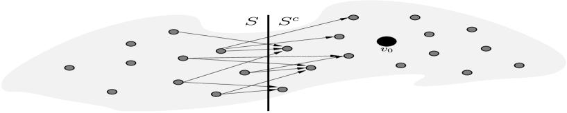
Figure 5: An artificial two-terminal system: all sources in $S$ are treated as a supersource, connected to a supersink made of all the sinks in $S^{c}$ by an array of DMCs (those going across the cut). Intuitively, any necessary condition for this system should also be necessary for our system (although this requires a formal statement and proof). The interesting statement thus is to show that the set of all conditions obtained in this form (by considering all possible cuts) is also sufficient.

Clearly, $H(U_{S}|U_{S^{c}})<\sum_{i\in S,j\in S^{c}}C_{ij}$ is an outer bound for this two-terminal system (follows directly from the source/channel separation theorem, [5, Sec. 8.13]). And intuitively, it is also clear that any outer bound for this two-terminal system provides necessary conditions for reliable communication to be possible in our network. Thus, by considering all possible partitions $(S,S^{c})$ as above, we obtain a set of necessary conditions matching those of the achievability result.

We would also like to highlight that, because of the correlation between sources, a simple max-flow/min-cut bounding argument as suggested in [5, Section 14.10]) is not sufficient to establish the source-channel separation result we seek – proving said result requires all the steps of a typical converse.

A formal proof for this converse is provided in Appendix -D.

II-D Special Cases

II-D1 A Network with Three Nodes

To provide an illustration of the meaning of Theorem 4, and of the optimality of the flow-based solution, we specialize Theorem 4 to the case of a network with three nodes. In this case, those conditions become:

$$H(U_{1}|U_{2}U_{0}) < C_{10}+C_{12}$$ (8)

$$H(U_{2}|U_{1}U_{0}) < C_{20}+C_{21}$$ (9)

$$H(U_{1}U_{2}|U_{0}) < C_{10}+C_{20}.$$ (10)

A network with three nodes as considered here is illustrated in Fig. 6.

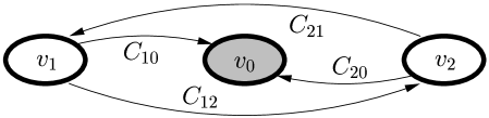
Figure 6: A network with three nodes.

Next, we regard the network in Fig. 6 as a flow network [34, Ch. 26]: a flow network with two sources ($v_{1}$ and $v_{2}$) and a single sink ($v_{0}$). Encodings of $U_{1}$ injected at source $v_{1}$ at rate $R_{1}$, and of $U_{2}$ injected at $v_{2}$ at rate $R_{2}$, are the “objects” that flow in this network and are to be delivered to the sink $v_{0}$. This is illustrated in Fig. 7.

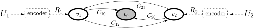
Figure 7: A flow network with three nodes, supplies $R_{1}$ and $R_{2}$ and nodes $v_{1}$ and $v_{2}$, and a sink $v_{0}$.

In the simple flow network of Fig. 7, any feasible flow $\varphi$ must satisfy some conservation equations:

$$\begin{array}[]{rclcl}R_{1}&=&\varphi(v_{1},v_{0})+\varphi(v_{1},v_{2}),\\ R_{2}&=&\varphi(v_{2},v_{0})+\varphi(v_{2},v_{1}),\\ R_{1}+R_{2}&=&\varphi(v_{1},v_{0})+\varphi(v_{1},v_{2})+\varphi(v_{2},v_{0})+\varphi(v_{2},v_{1})&=&\varphi(v_{1},v_{0})+\varphi(v_{2},v_{0}),\end{array}$$

where the last equality follows from the fact that flow conservation holds: the total amount of flow injected ($R_{1}+R_{2}$) must equal the total amount of flow received by the sink ($\varphi(v_{1},v_{0})+\varphi(v_{2},v_{0})$) [34]. Similarly, any feasible flow must also satisfy all capacity constraints:

$$\begin{array}[]{rcl}\varphi(v_{1},v_{0})+\varphi(v_{1},v_{2})&\leq&C_{10}+C_{12},\\ \varphi(v_{2},v_{0})+\varphi(v_{2},v_{1})&\leq&C_{20}+C_{21},\\ \varphi(v_{1},v_{0})+\varphi(v_{2},v_{0})&\leq&C_{10}+C_{20}.\end{array}$$

Combining these last two sets of constraints, and the conditions from the Slepian-Wolf theorem on feasible $(R_{1},R_{2})$ pairs, we immediately get

$$\begin{array}[]{rcccl}H(U_{1}|U_{2}U_{0})&<&R_{1}&\leq&C_{10}+C_{12},\\ H(U_{2}|U_{1}U_{0})&<&R_{2}&\leq&C_{20}+C_{21},\\ H(U_{1}U_{2}|U_{0})&<&R_{1}+R_{2}&\leq&C_{10}+C_{20}.\end{array}$$

It is interesting to observe in this argument that the region of achievable rates forms a convex polytope, in which three of its faces come from the Slepian-Wolf conditions, and three come from the capacity constraints. This polytope is illustrated in Fig. 8.

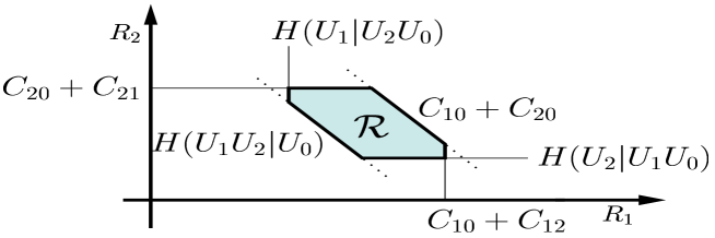
Figure 8: The polytope $\mathcal{R}$ of admissible rates.

This polytope plays a central role in our analysis: reliable communication is possible if and only if $\mathcal{R}\neq\emptyset$. Thus, the view of “information as a flow” in this class of networks is complete.

II-D2 No Cooperation and No Side Information at $v_{0}$

We consider now the special case of $M$ non-cooperating nodes and one sink, as illustrated in Fig. 9. Necessary and sufficient conditions for reliable communication under this scenario follow naturally from our main theorem by setting $C_{ij}=0$ for all $j\neq 0$, and $|\mathcal{U}_{0}|=1$.

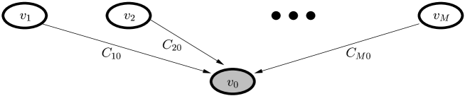
Figure 9: M non-cooperating nodes.

Corollary 1

The sources $U_{1},U_{2},\dots,U_{M}$ can be communicated reliably over an array of independent channels of capacity $C_{i0}$, $i=1\dots M$, if and only if

$$H(U_{S}|U_{S^{c}})<\sum_{i\in S}C_{i0},$$

for all subsets $S\subseteq\{1,2,\dots,M\}$, $S\neq\emptyset$.

An illustration of this corollary for two sources $U_{1}$ and $U_{2}$ is shown in Fig. 10.

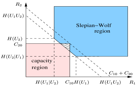
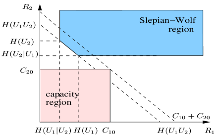
Figure 10: Relationship between the Slepian-Wolf region and the capacity region for two independent channels. In the left figure, as $H(U_{1}|U_{2})<C_{10}$ and $H(U_{2}|U_{1})<C_{20}$ the two regions intersect and therefore reliable communication is possible. The figure on the right shows the case in which $H(U_{2}|U_{1})>C_{20}$ and there is no intersection between the two regions.

When we have two independent channels with capacities $C_{10}$ and $C_{20}$, the capacity region becomes a rectangle with side lengths $C_{10}$ and $C_{20}$ [5, Chapter 14.3]. Also shown is the Slepian-Wolf region of achievable rates for separate encoding of correlated sources. Clearly, $H(U_{1}U_{2})<C_{10}+C_{20}$ is a necessary condition for reliable communication as a consequence of Shannon’s joint source and channel coding theorem for point-to-point communication. Assuming that this is the case, consider now the following possibilities:

• $H(U_{1})<C_{10}$ and $H(U_{2})<C_{20}$. The Slepian-Wolf region and the capacity region intersect, so any point $(R_{1},R_{2})$ in this intersection makes reliable communication possible. Alternatively, we can argue that reliable transmission of $U_{1}$ and $U_{2}$ is possible even with independent decoders, therefore a joint decoder will also achieve an error-free reconstruction of the source.

• $H(U_{1})>C_{10}$ and $H(U_{2})>C_{20}$. Since $H(U_{1}U_{2})<C_{10}+C_{20}$ there is always at least one point of intersection between the Slepian-Wolf region and the capacity region, so reliable communication is possible.

• $H(U_{1})<C_{10}$ and $H(U_{2})>C_{20}$ (or vice versa). If $H(U_{2}|U_{1})<C_{20}$ (or if $H(U_{1}|U_{2})<C_{10}$) then the two regions will intersect. On the other hand, if $H(U_{2}|U_{1})>C_{20}$ (or if $H(U_{1}|U_{2})>C_{10}$), then there are no intersection points, but it is not immediately clear whether reliable communication is possible or not (see Fig. 10), since examples are known in which the intersection between the capacity region of the multiple access channel and the Slepian-Wolf region of the correlated sources is empty and still reliable communication is possible [18].

Corollary 1 gives a definite answer to this last question: in the special case of correlated sources and independent channels an intersection between the capacity region and the Slepian-Wolf rate regions is not only sufficient, but also a necessary condition for reliable communication to be possible—in this case, separation holds.

II-D3 Arrays of Gaussian Channels

We should also mention that Theorem 4 applies to other channel models that are relevant in practice, for instance Gaussian channels with orthogonal multiple access. For simplicity, we illustrate this issue in the context of Corollary 1. The capacity of the Gaussian multiple access channel with $M$ independent sources is given by

$$\sum_{i\in S}R_{i}\leq\frac{1}{2}\log\left(1+\frac{\sum_{i\in S}P_{i}}{\sigma^{2}}\right),$$

for all $S\subseteq\{1...M\}$, $S\neq\emptyset$, and where $\sigma^{2}$ and $P_{i}$ are the noise power and the power of the $i$-th user respectively [5, pp. 378-379]. If we use orthogonal accessing (e.g. TDMA), and assign different time slots to each of the transmitters, then the Gaussian multiple access channel is reduced to an array of $M$ independent single-user Gaussian channels each with capacity

$$C_{i0}=\tau_{i0}\cdot\frac{1}{2}\log\bigg{(}1+\frac{P_{i0}}{\sigma^{2}\tau_{i0}}\bigg{)},\qquad 1\leq i\leq M,$$

where $\tau_{i0}$ is the time fraction allocated to source user $i$ to communicate with the data collector node $v_{0}$, and $P_{i0}$ is the corresponding power allocation.

Applying Theorem 4, we obtain the reachback capacity of the Gaussian channel with orthogonal accessing. Then, reliable communication is possible if and only if

$$H(U_{S}|U_{S^{c}})\leq\sum_{i\in S}\frac{\tau_{i0}}{2}\log\bigg{(}1+\frac{P_{i0}}{\sigma^{2}\tau_{i0}}\bigg{)},$$

for all subsets $S\subseteq\{1,2,\dots,M\}$, $S\neq\emptyset$.

III Practical/Engineering Implications of Theorem 4

III-A An Information Theoretically Optimal Protocol Stack

We believe that the fact that in networks of point-to-point noisy links with one sink Shannon information has the exact same properties of classical network flows is of particular practical relevance. This is so because there is a rich algorithmic theory associated with it, which allows us to cast standard information theoretic problems into the language of flows and optimization. Perhaps most relevant among these is is the optimality of implementing codes using a layered protocol stack, as illustrated in Fig. 11.

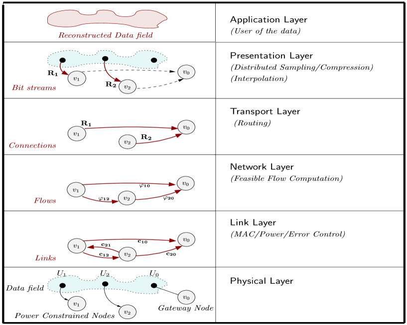
Figure 11: Abstractions that follow from the achievability proof, illustrated here for three nodes. At the physical layer there are nodes with power constraints, a data field of which these nodes collect samples in space and time, and a gateway node that will deliver all this data to destination. On top of this physical substrate, we construct a sequence of abstractions: noiseless point-to-point links of a given capacity (the Link Layer); a flow network (the Network Layer); a set of connections (the Transport Layer); and a set of distributed signal processing algorithms for sampling, compression and interpolation of the space/time continuous process (the Presentation Layer). In the end, an approximate representation of the underlying data field is delivered to applications.

As discussed in the Introduction, the decision to turn a wireless network into a network of point-to-point links is an arbitrary one. But, due to complexity and/or economic considerations, this arbitrary decision is one made very often, and thus we believe it is of great practical interest to understand what are appropriate design criteria for such networks. And our Theorem 4 offers valuable insights in this regard – if we decide to define a link-layer based on a MAC protocol that deals with interference by suppressing it, then all remaining layers in Fig. 11 follow from the achievability proof of Theorem 4. We see therefore that indeed, in this class of networks, Fig. 11 provides a set of abstractions analogous to those of Fig. 2 for classical two-terminal systems.

III-B Algorithmic/Computational Issues

As an illustration of the benefits of the “information as flow” interpretation for our results, in this subsection we outline some initial results on an optimal routing problem. This topic however will be developed in full depth elsewhere.

III-B1 Optimization Aspects of Protocol Design

A natural question that follows from our previous developments is one of optimization: given a non-empty feasibility polytope $\mathcal{R}$, we have the freedom of choosing among multiple assignments of values to flow variables, and thus it is only natural to ask if there is an optimal flow. To this end, we define a cost function $\kappa$ as follows:

$$\kappa(\varphi)=\sum_{(v_{i},v_{j})\in E}c(v_{i},v_{j})\cdot\varphi(v_{i},v_{j}),$$

where $c(v_{i},v_{j})$ is a constant that, multiplied by the total number of bits $\varphi(v_{i},v_{j})$ that a flow $\varphi$ assigns to an edge $(v_{i},v_{j})$, determines the cost of sending all that information over the channel $(\mathcal{X}_{ij},p_{ij}(y|x),\mathcal{Y}_{ij})$. The resulting optimization problem is shown in Fig. 12.

min       $\sum_{(v_{i},v_{j})\in E}\;\;c(v_{i},v_{j})\cdot\varphi(v_{i},v_{j})$   subject to: $$\begin{array}[]{lll}&\mbox{\tiny Standard flow constraints (capacity / skew symmetry / flow conservation)}\\ &\varphi(v_{i},v_{j})\leq C_{ij},&0\leq i,j\leq M.\\ &\varphi(v_{i},v_{j})=-\varphi(v_{j},v_{i}),&0\leq i,j\leq M.\\ &\sum_{v\in V}\varphi(v_{i},v)=0,&1\leq i\leq M.\\ &\mbox{\tiny Rate admissibility constraints}\\ &H(U_{S}|U_{S^{c}})<\sum_{i\in S}\varphi(s,v_{i})\leq\sum_{i\in S,j\in S^{c}}C_{ij},&S\subseteq\{1...M\},S\neq\emptyset.\\ &\varphi(s,v_{i})=R_{i},&1\leq i\leq M.\end{array}$$

Figure 12: Linear programming formulation for the assignment of values to flow variables (observe the introduction of a “supersource” $s$, which supplies $R_{i}$ units of flow to $v_{i}$). A solution to this problem provides optimal routes (those with positive flow assignment) and loads on each link. Note as well that, by choosing $c(v_{i},v_{j})=0$ for all $(v_{i},v_{j})\in E$, this LP is solvable if and only if $\mathcal{R}\neq\emptyset$ – that is, the decision problem for reliable communication (i.e., for whether a given load $p(U_{0}U_{1}...U_{M})$ can be carried over a given network $G$) admits a linear programming formulation too.

The choice of a linear cost model in this setup can be justified based on a number of reasons. First of all, linearity is a very natural assumption: in simple language, it says that it costs twice as much to double the amount of information sent on any channel. For example, we could take $c(v_{i},v_{j})$ to be the minimum energy per information bit required for reliable communication over the DMC from $v_{i}$ to $v_{j}$ [36], and then $\kappa(\varphi)$ would give us the sum of the energy consumed by all nodes when transporting data as dictated by a particular flow $\varphi$. Specifically in the context of routing problems, another important consideration is that the main drawback often cited for solving optimal routing problems based on network flow formulations is given by the fact that cost functions such as $\kappa$ only optimize average levels of link traffic, ignoring other traffic statistics [8, pg. 436]. But this is not at all an issue here, since the values of flow variables (i.e., Shannon information) are already average quantities themselves.

III-B2 A Routing Example

As one example of the usefulness of the LP formulation in Fig. 12, we consider next the problem of designing efficient mechanisms for data aggregation, as motivated in [37]. There has been a fair amount of work reported in the networking literature, on the design and performance analysis of tree structures for aggregation—for example, the work of Goel and Estrin on the construction of trees that perform well simultaneously under multiple concave costs [38]. Based on our LP formulation, we construct two examples which show the extent to which trees could give rise to suboptimalities, as opposed to other topological structures. And we start by showing an example in which, although $\mathcal{R}\neq\emptyset$, there are no feasible trees. This case is illustrated in Fig. 13.

Figure 13: To illustrate a solvable problem that cannot be solved using trees. Left: a flow network; middle/right: the decomposition of a feasible flow into two single flows, showing how much of the flow injected at each source is sent over which link ($x/c$ next to an edge means that the edge carries $x$ units of flow, and has capacity $c$).

As illustrated in Fig. 13, a solution to the transport problem exists. However, it is easy to check that if we constrain data to flow along trees, none of the three possible trees ($\{(v_{1},v_{0});(v_{2},v_{0})\}$, or $\{(v_{1},v_{2});(v_{2},v_{0})\}$, or $\{(v_{2},v_{1});(v_{1},v_{0})\}$) are feasible: in all cases, there is one link for which the capacity constraint is violated.

Next we consider a case where feasible trees exist, but the lowest cost of any tree differs from the optimal cost by an arbitrarily large factor. This case is illustrated in Fig. 14.

Figure 14: To illustrate a problem in which trees are very expensive. Left: a flow network with costs; right: an optimal solution to the linear program in Fig. 12. Such a case could arise, e.g., in a situation where there is heavy interference in the direct path from $v_{1}$ to $v_{0}$.

In this case, there exists only one feasible tree: $\{(v_{1},v_{0});(v_{2},v_{0})\}$, with cost $\ell(1+\epsilon)+1$. However, because of the “expensive” link $(v_{1},v_{0})$ along which the tree is forced to send all its data, the cost is significantly increased: by splitting the encoding of $U_{1}$ as illustrated in Fig. 14, the cost incurred into by this structure would be $\epsilon\ell+3$. Hence, we see that in this case, the cost of the best feasible tree is $\frac{\ell(1+\epsilon)+1}{\epsilon\ell+3}$ times larger than that of an optimal solution allowing splits. And this “overpayment factor” could be significant: when $\ell$ is large, this is $\approx 1+\frac{1}{\epsilon}$, and it grows unbound for small $\epsilon$.

Note as well that any time that a network is operated close to capacity, it will be necessary to split flows. And that is a situation likely to be encountered often in power-constrained networks, since minimum energy designs will necessarily result in links being allocated the least amount of power needed to carry a given traffic load. Thus, we see that these examples above are not pathological cases of limited practical interest, but instead, they are good representatives of situations likely to be encountered often in practice.

III-C Suboptimality of Correlated Codes for Orthogonal Channels

The key ingredient of the achievability proof presented by Cover, El Gamal and Salehi for the multiple access channel with correlated sources is the generation of random codes, whose codewords $X_{i}^{N}$ are statistically dependent on the source sequences $U_{i}^{N}$ [18]. This property, which is achieved by drawing the codewords according to $\prod_{j=1}^{N}p(x_{ij}|u_{ij})$ with $u_{ij}$ and $x_{ij}$ denoting the $j$-th element of $U_{i}^{N}$ and $X_{i}^{N}$, respectively, implies that $U_{i}^{N}$ and $X_{i}^{N}$ are jointly typical with high probability. Since the source sequences $U_{1}^{N}$ and $U_{2}^{N}$ are correlated, the codewords $X_{1}^{N}(U_{1}^{N})$ and $X_{2}^{N}(U_{2}^{N})$ are also correlated, and so we speak of correlated codes. This class of random codes, which is treated in more general terms in [21], can be viewed as joint source and channel codes that preserve the given correlation structure of the source sequences, based upon which the decoder can lower the probability of error.

The class of correlated codes is of interest to us because of two main reasons:

• From a practical point of view, correlated codes have a very strong appeal: sensor nodes with limited processing capabilities may be forced to use very simple codes that do not eliminate correlations between measurements prior to transmission [39] (e.g., a simple scalar quantizer and simple BPSK modulation).

• From a theoretical point of view, since these codes yield the largest known admissibility region for the problem of communicating distributed sources over multiple-access channels, it would be interesting to know how these codes fare in our context, where we know separate source and channel coding to achieve optimality.

Thus, specializing the achievability proof of [18] to the case of $M$ independent channels, we get the following result.

Corollary 2 (From Theorem 1 of [18])

A set of correlated sources $[U_{1}U_{2}...U_{M}]$ can be communicated reliably over independent channels $(\mathcal{X}_{1},p(y_{1}|x_{1}),\mathcal{Y}_{1})\dots(\mathcal{X}_{M},p(y_{M}|x_{M}),\mathcal{Y}_{M})$ to a sink $v_{0}$, if

$$H(U_{S}|U_{S^{c}})<\sum_{i\in S}I(X_{i};Y_{0}|U_{S^{c}}),$$

for all subsets $S\subseteq\{1,2,\dots,M\}$, $S\neq\emptyset$.

Proof:

This result can be obtained from the $M$-source version of the main theorem in  [18], by specializing it to a multiple access channel with conditional probability distribution

$$p(y|x_{1}x_{2}...x_{M})=p(y_{1}y_{2}\dots y_{M}|x_{1}x_{2}\dots x_{M})=\prod_{i=1}^{M}p(y_{i}|x_{i}).$$

∎

Part of the reason why we feel this is an interesting result is that the main theorem in [18] does not immediately specialize to Corollary 1: whereas the achievability results do coincide, [18] does not provide a converse. To illustrate this point better, we focus now on the case of $M=2$:

• In general, we have that $I(X_{1}X_{2};Y_{1}Y_{2})\leq I(X_{1};Y_{1})+I(X_{2};Y_{2})$, for any $p(u_{1}u_{2}x_{1}x_{2})p(y_{1}|x_{1})p(y_{2}|x_{2})$; but for this upper bound on the sum-rate to be achieved, we must take $p(u_{1}u_{2}x_{1}x_{2})=p(u_{1}u_{2})p(x_{1})p(x_{2})$ – that is, the codewords must be drawn independently of the source. And for this special case, our Theorem 4 does provide a converse.

• As argued earlier, due to practical considerations it may not be feasible to remove correlations in the source before choosing channel codewords, in which case we face a situation where correlated codes are used, despite their obvious suboptimality. In this case, it is of interest to determine the rate losses resulting from the use of correlated codes, defined as $\Delta_{1}=I(X_{1};Y_{1})-I(X_{1};Y_{1}|U_{2})$, $\Delta_{2}=I(X_{2};Y_{2})-I(X_{2};Y_{2}|U_{1})$, and $\Delta_{0}=I(X_{1};Y_{1})+I(X_{2};Y_{2})-I(X_{1}X_{2};Y_{1}Y_{2})$. Straightforward manipulations show that $\Delta_{1}=I(Y_{1};U_{2})$, $\Delta_{2}=I(Y_{2};U_{1})$, and $\Delta_{0}=I(Y_{1};Y_{2})$.

• Since $\Delta_{i}\geq 0$, $i\in\{0,1,2\}$ (mutual information is always nonnegative), we conclude that the region of achievable rates given by Corollary 2 is contained in the region defined by Corollary 1. Furthermore, we find that the rate loss terms have a simple, intuitive interpretation: $\Delta_{0}$ is the loss in sum rate due to the dependencies between the outputs of different channels, and $\Delta_{1}$ (or $\Delta_{2}$) represent the rate loss due to the dependencies between the outputs of channel $1$ (or $2$) and the source transmitted over channel $2$ (or $1$). All these terms become zero if, instead of using correlated codes, we fix $p(x_{1})p(x_{2})$ and remove the correlation between the source blocks before transmission over the channels.

At first glance, this observation may seem somewhat surprising, since the problem addressed by Corollary 1 is a special case of the multiple access channel with correlated sources considered in [18], where it is shown that in the general case correlated codes outperform the concatenation of Slepian-Wolf codes (independent codewords) and optimal channel codes. The crucial difference between the two problems is the presence (or absence) of interference in the channel. Albeit somewhat informally, we can state that correlated codes are advantageous when the transmitted codewords are combined in the channel through interference, which is obviously not the case in our problem. Practical code constructions built around this observation have been reported in [39].

IV Conclusions

IV-A Summary

In this paper we have considered the problem of encoding a set of distributed correlated sources for delivery to a single data collector node over a network of DMCs. For this setup we were able to obtain single-letter information theoretic conditions that provide an exact characterization of the admissibility problem. Two important conclusions follow from the achievability proof:

• Separate source/channel coding is optimal in any network with one sink in which interference is dealt with at the MAC layer by creating independent links among nodes.

• In such networks, the properties of Shannon information are exactly identical to those of water in pipes – information is a flow.

IV-B Discussion

A few interesting observations follow from our results:

• It is a well known fact that turning a multiple access channel into an array of orthogonal channels by using a suitable MAC protocol is a suboptimal strategy in general, in the sense that the set of rates that are achievable with orthogonal access is strictly contained in the Ahlswede-Liao capacity region [5, Ch. 14.3]. However, despite its inherent suboptimality, there are strong economic incentives for the deployment of networks based on such technologies, related to the low complexity and cost of existing solutions, as well as experience in the fabrication and operation of such systems. As a result, most existing standard implementations we are aware of (e.g., the IEEE 802.11 and 802.15.* families, or Bluetooth), are based on variants of protocols like TDMA/FDMA/CDMA or Aloha, that treat interference among users as noise or collisions, and deal with it by creating orthogonal links. We feel therefore that some of the interest in our results stems from the fact that they provide a thorough analysis for what we deem to be, with high likelihood, the vast majority of wireless communication networks to be deployed for the foreseeable future.

• A basic question follows from the results in this paper: when exactly does Shannon information act like a classical flow in a network setup? In this paper, we showed that far more often than common wisdom would suggest: for any network made up of independent links and one sink, Shannon information is a flow. The assumption of independence among channels is crucial, since well known counterexamples hold without it [18]. But, as argued before, far from being just some technical assumption needed for the theory to hold, independent channels arise naturally in practical applications. In establishing the flow properties of information, we showed how some well understood network flow tools can be applied to address network design problems that have traditionally been difficult to deal with using standard tools in network information theory, and we illustrated this with a simple example involving optimal routing. In particular we showed that, at least from an information theoretic point of view, there is little justification for the common practice of designing trees for collecting data picked up by a sensor network, thus opening up interesting problems of protocol design.

• In retrospect, perhaps the results we prove in this paper should not have been surprising. In the context of two-terminal networks, we do know the following:

  • Feedback does not increase the capacity. Therefore, the capacity of individual links is unaffected by the ability of our codes to establish a conference mechanism among nodes.

  • Compression rates are not reduced by explicit cooperation, as it follows from the Slepian-Wolf theorem: the minimum rate required to communicate $U_{1}$ to a decoder that has access to side-information $U_{0}$ is $H(U_{1}|U_{0})$, and knowledge of $U_{0}$ does not reduce the rates needed for coding $U_{1}$. Therefore, the amount of information that needs to flow through our network is not reduced either by the ability of nodes to establish conferences.

  Of course the statements above only hold for individual links, and a proof was needed to carry that intuition to the general network setup considered in this work. But those observations we think are the key to understanding why our results hold.

IV-C Future Work

After having established coding theorems for the problem of network information flow with correlated sources, a natural question that arises: what if, in a given scenario, $\mathcal{R}=\emptyset$? In that case, the best we can hope for is to reconstruct an approximation to the original source message — and the answer is given by rate-distortion theory [40]. The rate-distortion formulation of our problem in the case of non-cooperating encoders is equivalent to the well known (and still open) Multiterminal Source Coding problem [12]. Our current efforts are focused on completing work on the rate/distortion problem, and on fully developing the ideas outlined in Section III-B (e.g., to deal with problems of the type considered in [41]).

References

- [1] J. Barros and S. D. Servetto. On the Capacity of the Reachback Channel in Wireless Sensor Networks. In Proc. IEEE Int. Workshop Multimedia Sig. Proc., US Virgin Islands, 2002. Invited paper to the special session on Signal Processing for Wireless Networks.
- [2] J. Barros and S. D. Servetto. Reachback Capacity with Non-Interfering Nodes. In Proc. IEEE Int. Symp. Inform. Theory (ISIT), Yokohama, Japan, 2003.
- [3] J. Barros and S. D. Servetto. Coding Theorems for the Sensor Reachback Problem with Partially Cooperating Nodes. In Discrete Mathematics and Theoretical Computer Science (DIMACS) series on Network Information Theory, Piscataway, NJ, 2003.
- [4] J. Barros and S. D. Servetto. A Coding Theorem for Network Information Flow with Correlated Sources. In Proc. IEEE Int. Symp. Inform. Theory (ISIT), Adelaide, Australia, 2005.
- [5] T. M. Cover and J. Thomas. Elements of Information Theory. John Wiley and Sons, Inc., 1991.
- [6] I. F. Akyildiz, W. Su, Y. Sankarasubramaniam, and E. Cayirci. A Survey on Sensor Networks. IEEE Communications Mag., 40(8):102–114, 2002.
- [7] T. Berger, Z. Zhang, and H. Viswanathan. The CEO Problem. IEEE Trans. Inform. Theory, 42(3):887–902, 1996.
- [8] D. Bertsekas and R. Gallager. Data Networks (2nd ed). Prentice Hall, 1992.
- [9] A. Hu and S. D. Servetto. dFSK: Distributed Frequency Shift Keying Modulation in Dense Sensor Networks. In Proc. IEEE Int. Conf. Commun. (ICC), Paris, France, 2004.
- [10] A. Hu and S. D. Servetto. Algorithmic Aspects of the Time Synchronization Problem in Large-Scale Sensor Networks. ACM/Kluwer Mobile Networks and Applications, 10:491–503, 2005. Special issue with selected (and revised) papers from ACM WSNA 2003.
- [11] A. Hu and S. D. Servetto. On the Scalability of Cooperative Time Synchronization in Pulse-Connected Networks. IEEE Trans. Inform. Theory, to appear. Available from http://cn.ece.cornell.edu/.
- [12] T. Berger. The Information Theory Approach to Communications (G. Longo, ed.), chapter Multiterminal Source Coding. Springer-Verlag, 1978.
- [13] I. Csiszár and J. Körner. Towards a General Theory of Source Networks. IEEE Trans. Inform. Theory, 26(2):155–166, 1980.
- [14] J. Körner and K. Marton. How to Encode the Modulo-Two Sum of Binary Sources. IEEE Trans. Inform. Theory, 25(2):219–221, 1979.
- [15] V. Kawadia and P. R. Kumar. A Cautionary Perspective on Cross-Layer Design. IEEE Wireless Comm. Mag., 2004. Available from http://decision.csl.uiuc.edu/~prkumar/.
- [16] A. Ephremides and B. Hajek. Information Theory and Communication Networks: An Unconsummated Union. IEEE Trans. Inform. Theory, 44(6):2416–2434, 1998.
- [17] D. Slepian and J. K. Wolf. Noiseless Coding of Correlated Information Sources. IEEE Trans. Inform. Theory, IT-19(4):471–480, 1973.
- [18] T. M. Cover, A. A. El Gamal, and M. Salehi. Multiple Access Channels with Arbitrarily Correlated Sources. IEEE Trans. Inform. Theory, IT-26(6):648–657, 1980.
- [19] G. Dueck. A Note on the Multiple Access Channel with Correlated Sources. IEEE Trans. Inform. Theory, IT-27(2):232–235, 1981.
- [20] D. Slepian and J. K. Wolf. A Coding Theorem for Multiple Access Channels with Correlated Sources. Bell Syst. Tech. J., 52(7):1037–1076, 1973.
- [21] R. Ahlswede and T. S. Han. On Source Coding with Side Information via a Multiple-Access Channel, and Related Problems in Multi-User Information Theory. IEEE Trans. Inform. Theory, 29(3):396–411, 1983.
- [22] F. M. J. Willems. The Discrete Memoryless Multiple Access Channel with Partially Cooperating Encoders. IEEE Trans. Inform. Theory, 29(3):441–445, 1983.
- [23] T. S. Han. Slepian-Wolf-Cover Theorem for a Network of Channels. Inform. Contr., 47(1):67–83, 1980.
- [24] R. Ahlswede, N. Cai, S.-Y. R. Li, and R. W. Yeung. Network Information Flow. IEEE Trans. Inform. Theory, 46(4):1204–1216, 2000.
- [25] S. Borade. Network Information Flow: Limits and Achievability. In Proc. IEEE Int. Symp. Inform. Theory (ISIT), Lausanne, Switzerland, 2002.
- [26] S.-Y. R. Li, R. W. Yeung, and N. Cai. Linear Network Coding. IEEE Trans. Inform. Theory, 49(2):371–381, 2003.
- [27] R. Koetter and M. Médard. An Algebraic Approach to Network Coding. IEEE/ACM Trans. Networking, 11(5):782–795, 2003.
- [28] M. Effros, M. Médard, T. Ho, S. Ray, D. Karger, and R. Koetter. Linear Network Codes: A Unified Framework for Source, Channel, and Network Coding. In Discrete Mathematics and Theoretical Computer Science (DIMACS) series on Network Information Theory, Piscataway, NJ, 2003.
- [29] T. Ho, M. Médard, M. Effros, and R. Koetter. Network Coding for Correlated Sources. In Proc. 38th Annual Conf. Inform. Sciences Syst. (CISS), Princeton, NJ, March 2004.
- [30] Z. Li and B. Li. Network Coding in Undirected Networks. In Proc. 38th Annual Conf. Inform. Sciences Syst. (CISS), Princeton, NJ, March 2004.
- [31] P. Gupta and P. R. Kumar. The Capacity of Wireless Networks. IEEE Trans. Inform. Theory, 46(2):388–404, 2000.
- [32] C. Peraki and S. D. Servetto. On the Maximum Stable Throughput Problem in Random Networks with Directional Antennas. In Proc. ACM MobiHoc, Annapolis, MD, 2003.
- [33] C. Peraki and S. D. Servetto. Capacity, Stability and Flows in Large-Scale Random Networks. In Proc. IEEE Inform. Theory Workshop (ITW), San Antonio, TX, 2004.
- [34] T. H. Cormen, C. E. Leiserson, R. L. Rivest, and C. Stein. Introduction to Algorithms (2nd ed). MIT Press, 2001.
- [35] A. R. Lehman and E. Lehman. Complexity Classification of Network Information Flow Problems. In Proc. ACM/SIAM Symp. Discr. Alg. (SODA), 2004.
- [36] S. Verdú. Spectral Efficiency in the Wideband Regime. IEEE Trans. Inform. Theory, 48(6):1319–1343, 2002.
- [37] C. Intanagonwiwat, R. Govindan, D. Estrin, J. Heidemann, and F. Silva. Directed Diffusion for Wireless Sensor Networking. IEEE/ACM Trans. Networking, 11(1):2–16, 2003.
- [38] A. Goel and D. Estrin. Simultaneous Optimization for Concave Costs: Single Sink Aggregation or Single Source Buy-at-Bulk. In Proc. ACM/SIAM Symp. Discr. Alg. (SODA), Baltimore, MD, 2003.
- [39] J. Barros, M. Tüchler, and S. P. Lee. Scalable Source/Channel Decoding for Large-Scale Sensor Networks. In Proc. Int. Conf. Commun. (ICC), Paris, France, 2004.
- [40] T. Berger. Rate Distortion Theory: A Mathematical Basis for Data Compression. Prentice-Hall, Inc., 1971.
- [41] M. Chiang. Balancing Transport and Physical Layers in Wireless Multihop Networks: Jointly Optimal Congestion Control and Power Control. IEEE. J. Select. Areas Commun., 23(1):104–116, 2005.