Bandit Problems with Side Observations

Abstract

An extension of the traditional two-armed bandit problem is considered, in which the decision maker has access to some side information before deciding which arm to pull. At each time $t$, before making a selection, the decision maker is able to observe a random variable $X_{t}$ that provides some information on the rewards to be obtained. The focus is on finding uniformly good rules (that minimize the growth rate of the inferior sampling time) and on quantifying how much the additional information helps. Various settings are considered and for each setting, lower bounds on the achievable inferior sampling time are developed and asymptotically optimal adaptive schemes achieving these lower bounds are constructed.

I Introduction

Since the publication of [1], bandit problems have attracted much attention in various areas of statistics, control, learning, and economics (e.g., see [2, 3, 4, 5, 6, 7, 8, 9, 10]). In the classical two-armed bandit problem, at each time a player selects one of two arms and receives a reward drawn from a distribution associated with the arm selected. The essence of the bandit problem is that the reward distributions are unknown, and so there is a fundamental trade-off between gathering information about the unknown reward distributions and choosing the arm we currently think is the best. A rich set of problems arises in trying to find an optimal/reasonable balance between these conflicting objectives (also referred to as learning versus control, or exploration versus exploitation).

We let $\{Y^{1}_{\tau}\}$ and $\{Y^{2}_{\tau}\}$ denote the sequences of rewards from arms 1 and 2 in a two-armed bandit machine. In the traditional parametric setting, the underlying configurations/distributions of the arms are expressed by a pair of parameters $C_{0}=(\theta_{1},\theta_{2})$ such that $\{Y^{1}_{\tau}\}$ and $\{Y^{2}_{\tau}\}$ are independent and identically distributed (i.i.d.) with distribution $(F_{\theta_{1}},F_{\theta_{2}})$, where $\{F_{\theta}\}$ is a known family of distributions parametrized by $\theta$. The goal is to maximize the sum of the expected rewards. Results on achievable performance have been obtained for a number of variations and extensions of the basic problem defined in [9] (e.g., see [11, 12, 13, 14, 15, 16, 17]).

In this paper, we consider an extension of the classical two-armed bandit where we have access to side information before making our decision about which arm to pull. Suppose at time $t$, in addition to the history of previous decisions, outcomes, and observations, we have access to a side observation $X_{t}$ to help us make our current decision. The extent to which this side observation can help depends on the relationship of $X_{t}$ to the reward distributions of $Y^{1}_{t}$ and $Y^{2}_{t}$.

Previous work on bandit problems with side observations includes [18, 19, 20, 21, 22]. Woodroofe [21] considered a one-armed bandit in a Bayesian setting, and constructed a simple criterion for asymptotically optimal rules. Sarkar [20] extended the side information model of [21] to the exponential family. In [19], Kulkarni considered classes of reward distributions and their effects on performance using results from learning theory. Most of the previous work with side observations is on one-armed bandit problems, which can be viewed as a special case of the two-armed setting by letting arm 2 always return zero.

In contrast with this previous work, we consider various general settings of side information for a two-armed bandit problem. Our focus is on providing both lower bounds and bound-achieving algorithms for the various settings. The results and proofs are very much along the lines of [8] and subsequent works as in [11, 12, 13, 14, 15].

We now describe the settings considered in this paper.

1. Direct Information: In this case, $X_{t}$ provides information directly about the underlying configuration $C_{0}=(\theta_{1},\theta_{2})$, which allows a type of separation between the learning and control. This has a dramatic effect on the achievable inferior sampling time. Specifically, estimating $(\theta_{1},\theta_{2})$ by observing $\{X_{\tau}\}$, and using the estimate $(\hat{\theta}_{1},\hat{\theta}_{2})$ to make the decision, results in bounded expected inferior sampling time.

If the distribution of $\{X_{\tau}\}$ is not a function of $C_{0}$, we are not able to learn $C_{0}$ through $\{X_{\tau}\}$. However, different values of the side observation $X_{t}$ will result in different conditional distributions of the rewards $Y^{i}_{t}$. By exploiting this new structure (observing $X_{t}$ in advance), we can hope to do better than the case without any side observation.

A physical meaning about the above scenario (constant distribution on $\{X_{\tau}\}$) is that a two-armed bandit with the side observations drawn from a finite set $\{x_{1},x_{2},\cdots,x_{n}\}$ can be viewed as a set of $n$ different two-armed sub-bandit machines indexed from $x_{1}$ to $x_{n}$. The player does not know the order of sub-machines he is going to play, which is determined by rolling a die with $n$ faces. However, by observing $X_{t}$, the player knows which machine (out of the $n$ different ones) he is facing now before selecting which arm to play. The connection between these sub-machines is that they share the same common configuration pair $(\theta_{1},\theta_{2})$, so that the rewards observed from one machine provide information on the common $(\theta_{1},\theta_{2})$, which can then be applied to all of the others (different values of $X_{t}$). This is the key aspect that makes this setup distinct from simply having many independent bandit problems with random access opportunity.

We consider the following three cases of different relationships among the most rewarding arm, $C_{0}$, and $X_{t}$.

1. For all possible $C_{0}$, the best arm is a function of $X_{t}$: That is, $\forall(\theta_{1},\theta_{2}),\exists x_{1},x_{2}$ such that at time $t$, arm 1 yields higher expected reward conditioned on $X_{t}=x_{1}$ while arm 2 is preferred when $X_{t}=x_{2}$. Surprisingly, we exhibit an algorithm that achieves bounded expected inferior sampling time in this case. Woodroofe’s result [21] can then be viewed as a special case of this scenario.

2. For all possible $C_{0}$, the best arm is not a function of $X_{t}$: In this case, for all configurations $(\theta_{1},\theta_{2})$, one of the arms is always preferred regardless of the value of $X_{t}$. Since the conditional reward distributions are functions of $X_{t}$, the intuition is that we can postpone our learning until it is most advantageous to us. We show that, asymptotically, our performance will be governed by the most “informative” bandit (among the different values taken on by $X_{t}$).

3. Mixed Case: This is a general case that combines the previous two, and contains the main contribution of this paper. For some possible configurations, one arm may always be preferred (for any $X_{t}$), while for other possible configurations, the preferred arm is a function of $X_{t}$. We exhibit an algorithm that achieves the best possible in either case. That is, if the best arm is a function of $X_{t}$, it achieves bounded expected inferior sampling time as in Case 2, while if the underlying configuration is such that one arm is always preferred, then we get the results of Case 3.

Our paper is organized as follows. In Section II, we introduce the general formulation. In Section III, we provide background on the asymptotic analysis of traditional bandit problems (without side observations). In Sections IV through VII, we consider the above four cases respectively. The results are included in each section, while details of the proofs are provided in the appendix.

II General Formulation

Consider the two-armed bandit problem defined as follows. Suppose we have two sequences of (real-valued) random variables (r.v.’s), $\{Y^{i}_{\tau}\}_{i=1,2}$, and an i.i.d. side observation sequence $\{X_{\tau}\}$, taking values in ${\mathbf{X}}\subset{\mathbb{R}}$. $\{Y^{i}_{\tau}\}$ denotes the reward sequence of arm $i$ while $X_{t}$ is the side information observed at time $t$ before making the decision. The formal parametric setting is as follows. For each configuration pair $C_{0}=(\theta_{1},\theta_{2})$ and each $i$, the sequence of vectors $(X_{t},Y^{i}_{t})$ is i.i.d. with joint distribution $G_{C_{0}}(dx)F_{\theta_{i}}(dy|x)$, where the families $\{G_{C}\}_{C\in{\mathbf{\Theta}}^{2}}$ and $\{F_{\theta}(\cdot|\cdot)\}_{\theta\in{\mathbf{\Theta}}}$ are known to the player, but the true value of the corresponding index $C_{0}$ must be learned through experiments. For notational simplicity, we further assumed ${\mathbf{\Theta}}$ is a set of real numbers.

TABLE I: Glossary

Not’n	Description
$G_{C}(dx)$	The marginal distribution of the i.i.d. $\{X_{\tau}\}$ under configuration $C$.
$F_{\theta_{i}}(dy|x)$	The conditional distribution of the reward of arm $i$, $Y^{i}_{t}$, under parameter $\theta_{i}$.
$\mu_{\theta}(x)$	The conditional expectation of the reward, $\mu_{\theta}(x)={\mathsf{E}}_{\theta}\{Y|x\}=\int yF_{\theta}(dy|x)$.
$1(C_{0})$, $2(C_{0})$	The first and the second coordinates of the configuration pair $C_{0}$, i.e. $1(C_{0})=\theta_{1}$, $2(C_{0})=\theta_{2}$. For example: $F_{1(C_{0})}(dy|x)=F_{\theta_{1}}(dy|x)$ and $\mu_{2(C_{0})}(x)=\mu_{\theta_{2}}(x)$.
$M_{C}(x)$	The index of the preferred arm, i.e. $\arg\max_{i=1,2}\{\mu_{i(C)}(x)\}$.
$\phi_{t}$	The decision rule taking values in $\{1,2\}$ and depending only on the past outcomes and the current side information $X_{t}$.
$T_{i}(t)$	The total number of samples taken on arm $i$ up to time $t$, $T_{i}(t)=\sum^{t}_{\tau=1}1_{\{\phi_{\tau}=i\}}$.
$T_{inf}(t)$	The total number of samples taken on the inferior arm up to time $t$: $T_{inf}(t)=\sum^{t}_{\tau=1}1_{\{\phi_{\tau}\neq M_{C_{0}}(X_{\tau})\}}$.
$I(P,Q)$	The Kullback-Leibler (K-L) information number between distributions $P$ and $Q$: $I(P,Q)={\mathsf{E}}_{P}\left\{\log\left(\frac{dP}{dQ}\right)\right\}$.
$I(\theta_{1},\theta_{2}|x)$	The conditional K-L information number: $I(\theta_{1},\theta_{2}|x)=I(F_{\theta_{1}}(\cdot|x),F_{\theta_{2}}(\cdot|x))$.

Note that the concept of the i.i.d. bandit is now extended to the assumption that the vector sequence $\{(X_{t},Y^{i}_{t})\}_{t}$ is i.i.d. The unconditioned marginal sequence $\{Y^{i}_{\tau}\}$ remains i.i.d. However, rather than the unconditional marginals, the player is now facing the conditional distribution of $Y^{i}_{t}$, which is a function of the observed side information $X_{t}$ (and is not identically distributed given different $X_{t}$).

The goal is to find an adaptive allocation rule $\{\phi_{\tau}\}$ to maximize the growth rate of the expected reward:

$${\mathsf{E}}_{C_{0}}\{W_{\phi}(t)\}:={\mathsf{E}}_{C_{0}}\left\{\sum^{t}_{\tau=1}\left(1_{\{\phi_{\tau}=1\}}Y^{1}_{\tau}+1_{\{\phi_{\tau}=2\}}Y^{2}_{\tau}\right)\right\},$$

or equivalently to minimize the growth rate of the expected inferior sampling time, namely ${\mathsf{E}}_{C_{0}}\{T_{inf}(t)\}$. To be more explicit, at any time $t$, $\phi_{t}$ takes a value in $\{1,2\}$ and depends only on the past rewards ($\tau<t$) and the current side observation $X_{t}$.

We define a uniformly good rule as follows.

Definition 1 (Uniformly Good Rules)

An allocation rule $\{\phi_{\tau}\}$ is uniformly good if for all $C\in{\mathbf{\Theta}}^{2}$, ${\mathsf{E}}_{C}\{T_{inf}(t)\}=o(t^{\alpha})$, $\forall\alpha>0$.

In what follows, we consider only uniformly good rules and regard other rules as uninteresting. Necessary notation and several quantities of interest are defined in TABLE I. We assume that all the given expectations exist and are finite.

III Traditional Bandits

Under the general formulation provided in Section II, the traditional non-Bayesian, parametric, infinite horizon, two-armed bandit is simply a degenerate case, i.e., the traditional bandit problem is equivalent to having only one element in $\mathbf{X}$ (say ${\mathbf{X}}=\{x_{0}\}$). This formulation of traditional bandit problems is identical to the two-armed case of [14, 8, 9]. For simplicity, the argument $x_{0}$ can be omitted in this traditional setting, i.e., $M_{C}:=M_{C}(x_{0})$, $\mu_{\theta}:=\mu_{\theta}(x_{0})$, $I(\theta_{1},\theta_{2}):=I(\theta_{1},\theta_{2}|x_{0})$, etc.

The main contribution of [14, 8, 9] is the asymptotic analysis stated as the following two theorems.

Theorem 1 ($\log t$ Lower Bound)

For any uniformly good rule $\{\phi_{\tau}\}$, $T_{inf}(t)$ satisfies

$$\lim_{t\rightarrow\infty}{\mathsf{P}}_{C_{0}}\left(T_{inf}(t)\geq\frac{(1-\epsilon)\log t}{K_{C_{0}}}\right)=1,~{}\forall\epsilon>0,$$

and $$\liminf_{t\rightarrow\infty}\frac{{\mathsf{E}}_{C_{0}}\{T_{inf}(t)\}}{\log t}\geq\frac{1}{K_{C_{0}}},$$

where $K_{C_{0}}$ is a constant depending on $C_{0}$. If $M_{C_{0}}=2$, then $T_{inf}(t)=T_{1}(t)$ and $K_{C_{0}}$ is defined as follows.

$$K_{C_{0}}=\inf\{I(\theta_{1},\theta):\forall\theta,\mu_{\theta}>\mu_{\theta_{2}}\}.$$ (1)

The expression for $K_{C_{0}}$ for the case in which $M_{C_{0}}=1$ can be obtained by symmetry.

Theorem 2 (Asymptotic Tightness)

Under certain regularity conditions, the above lower bound is asymptotically tight. Formally stated, given the distribution family $\{F_{\theta}\}$, there exists a decision rule $\{\phi_{\tau}\}$ such that for all $C_{0}=(\theta_{1},\theta_{2})\in{\mathbf{\Theta}}^{2}$,

$$\limsup_{t\rightarrow\infty}\frac{{\mathsf{E}}_{C_{0}}\{T_{inf}(t)\}}{\log t}\leq\frac{1}{K_{C_{0}}},$$

where $K_{C_{0}}$ is the same as in Theorem 1.

The intuition behind the $\log t$ lower bound is as follows. Suppose $M_{C_{0}}=2$ and consider another configuration $C^{\prime}=(\theta,\theta_{2})$ such that $M_{C^{\prime}}=1$. It can be shown that if under configuration $C_{0}=(\theta_{1},\theta_{2})$, ${\mathsf{E}}_{C_{0}}\{T_{inf}(t)\}$ is less than the $\log t$ lower bound, ${\mathsf{E}}_{C^{\prime}}\{T_{inf}(t)\}$ must be greater than $o(t^{\alpha})$ for some $\alpha>0$, which contradicts the assumption that $\{\phi_{\tau}\}$ is uniformly good.

IV Direct Information

IV-A Formulation

In this setting, the side observation $X_{t}$ directly reveals information about the underlying configuration pair $C_{0}=(\theta_{1},\theta_{2})$ in the following way.

Dependence:

$G_{C_{1}}=G_{C_{2}}$ iff $C_{1}=C_{2}$.

As a result, observing the empirical distribution of $X_{t}$ gives us useful information about the underlying parameter pair $C_{0}$. Thus this is a type of identifiability condition.

Examples:

• ${\mathbf{\Theta}}=(0,0.5)$ and ${\mathbf{X}}=\{x_{1},x_{2},x_{3}\}$.

  $${\mathsf{P}}_{(\theta_{1},\theta_{2})}(X_{t}=x_{k})=\begin{cases}\theta_{k}&\text{if $k=1,2$}\\ 1-\theta_{1}-\theta_{2}&\text{otherwise}\end{cases}.$$

• ${\mathbf{\Theta}}=(0,\infty)$ and ${\mathbf{X}}=[0,1]$. $X_{t}$ is beta distributed with parameters $(\theta_{1},\theta_{2})$.

IV-B Scheme with Bounded ${\mathsf{E}}_{C_{0}}\{T_{inf}(t)\}$

Consider the following condition.

Condition 1

For any fixed $C_{0}$

$$\inf\left\{\rho(G_{C_{0}},G_{C_{e}}):C_{e}\in{\mathbf{\Theta}^{2}},\exists x,M_{C_{e}}(x)\neq M_{C_{0}}(x)\right\}>0,$$

where $\rho$ denotes the Prohorov metric on the space of distributions. Two examples satisfying Condition 1 are as follows:

• Example 1: $\mathbf{X}$ is finite, and $\forall x\in\mathbf{X}$, $\mu_{\theta}(x)$ is continuous with respect to (w.r.t.) $\theta$.

• Example 2: $F_{\theta}(\cdot|x)\sim{\mathcal{N}}(\theta x,1)$ is a Gaussian distribution with mean $\theta x$ and variance $1$.

Under this condition, we obtain the following result.

Theorem 3 (Bounded ${\mathsf{E}}_{C_{0}}\{T_{inf}(t)\}$)

If Condition 1 is satisfied, then there exists an allocation rule $\{\phi_{\tau}\}$, such that $\lim_{t\rightarrow\infty}{\mathsf{E}}_{C_{0}}\{T_{inf}(t)\}<\infty$ and $\lim_{t\rightarrow\infty}T_{inf}(t)<\infty$ a.s.

• Note: the information directly revealed by $X_{t}$ helps the sequential control scheme surpass the $\log t$ lower bound stated in Theorem 1. This significant improvement (bounded expected inferior sampling time) is due to the fact that the dilemma between learning and control no longer exists in the direct information case.

We provide a scheme achieving bounded ${\mathsf{E}}_{C_{0}}\{T_{inf}(t)\}$ as in Algorithm 1, of which a detailed analysis is given in Appendix B.

Algorithm 1 $\phi_{t}$, the decision at time $t$ (after observing $X_{t}$ but before deciding $\phi_{t}$)

1:  Construct

$${\mathbf{C}}_{t}:=\left\{C\in{\mathbf{\Theta}}^{2}:\rho(G_{C},L_{X}(t))\leq\inf_{C\in{\mathbf{\Theta}}^{2}}\rho(G_{C},L_{X}(t))+\frac{1}{t}\right\},$$

where $L_{X}(t)$ is the empirical measure of the side observations $\{X_{\tau}\}$ until time $t$, and $\rho$ is the Prohorov metric as before.

2:  Arbitrarily pick $\hat{C}_{t}\in{\mathbf{C}}_{t}$, and set $\phi_{t}=M_{\hat{C}_{t}}(X_{t})$.

V Best Arm As A Function Of $X_{t}$

For all of the following sections (Sections V through VII), we consider only the case in which observing $X_{t}$ will not reveal any information about $C_{0}$, but only reveals information about the upcoming reward $Y^{i}_{t}$, that is,

• $G_{C_{0}}$ does not depend on the value of $C_{0}$; we use $G:=G_{C_{0}}$ as shorthand notation.

Three further refinements regarding the relationship between $M_{C}(x)$ and $x$ will be discussed separately (each in one section).

V-A Formulation

In this section, we assume that for all possible $C$, the side observation $X_{t}$ is always able to change the preference order as shown in Fig. 1. That is,

• For all $C\in{\mathbf{\Theta}}^{2}$, there exist $x_{1}$ and $x_{2}$ such that $M_{C}(x_{1})=1$ and $M_{C}(x_{2})=2$.

Figure 1: The best arm at time $t$ always depends on the side observation $X_{t}$. That is, for any possible pair $(\theta_{1},\theta_{2})$ the two curves, $\mu_{\theta_{1}}(x)$ and $\mu_{\theta_{2}}(x)$, (w.r.t. $x$) always intersect each other.

The needed regularity conditions are as follows.

1. ${\mathbf{X}}$ is a finite set and ${\mathsf{P}}_{G}(X_{t}=x)>0$ for all $x\in{\mathbf{X}}$.

2. $\forall\theta_{1},\theta_{2},x$, $I(\theta_{1},\theta_{2}|x)$ is strictly positive and finite.

3. $\forall x$, $\mu_{\theta}(x)$ is continuous w.r.t. $\theta$.

The first condition embodies the idea of treating $X_{t}$ as the index of several different bandit machines, which also simplifies our proof. The second condition is to ensure that all these different bandit problems are non-trivial, with non-identical pairs of arms.

Example:

• ${\mathbf{\Theta}}=(0,\infty)$, ${\mathbf{X}}=\{-1,1\}$, and the conditional reward distribution $F_{\theta}(\cdot|x)\sim{\mathcal{N}}(\theta x,1)$.

V-B Scheme with Bounded ${\mathsf{E}}_{C_{0}}\{T_{inf}(t)\}$

Theorem 4 (Bounded ${\mathsf{E}}_{C_{0}}\{T_{inf}(t)\}$)

If the above conditions are satisfied, there exists an allocation rule $\{\phi_{\tau}\}$ such that

$$\lim_{t\rightarrow\infty}{\mathsf{E}}_{C_{0}}\{T_{inf}(t)\}<\infty.$$

Such a rule is obviously uniformly good.

• Note: although the side observation $X_{t}$ does not reveal any information about $C_{0}$ in this setting, the alternation of the best arm as the i.i.d.  $X_{t}$ takes on different values $x$ makes it possible to always perform the control part, $\phi_{t}=M_{\hat{C}_{t-1}}(X_{t})$, and simultaneously sample both arms often enough. Since the information about both arms will be implicitly revealed (through the alternation of $M_{C_{0}}(X_{t})$), the dilemma of learning and control no longer exists, and a significant improvement ($\lim_{t\rightarrow\infty}{\mathsf{E}}_{C_{0}}\{T_{inf}(t)\}<\infty$) is obtained over the $\log t$ lower bound in Theorem 1.

Algorithm 2 $\phi_{t}$, the decision at time $t+1$

Variables: Denote $T_{i}^{x}(t)$ as the total number of time instants until time $t$ when arm $i$ has been pulled and $X_{\tau}=x$, i.e.

$$T_{i}^{x}(t):=\sum_{\tau=1}^{t}1_{\{X_{\tau}=x,\phi_{\tau}=i\}},$$

and define $x^{\star}_{i}:=\arg\max_{x}\left\{T_{i}^{x}(t)\right\}$ and $T^{x^{\star}}_{i}(t):=\max_{x}\left\{T_{i}^{x}(t)\right\}$.

Construct

$${\mathbf{C}}_{t} := \{C=(\theta_{1},\theta_{2})\in{\mathbf{\Theta}}^{2}:$$

$$~{}~{}\sigma(C,t)\leq\inf\{\sigma(C,t):C\in{\mathbf{\Theta}}^{2}\}+\frac{1}{t}\},$$

$$\mbox{with~{}~{}~{}~{}~{}~{}~{}~{}~{}~{}}\sigma(C,t) := \rho(F_{1(C)}(\cdot|x^{\star}_{1}),L_{1}^{x^{\star}}(t)),~{}~{}~{}~{}~{}~{}~{}~{}~{}~{}~{}~{}~{}~{}~{}~{}~{}~{}~{}~{}~{}~{}~{}~{}~{}~{}$$

$$+\rho(F_{2(C)}(\cdot|x_{2}^{\star}),L_{2}^{x^{\star}}(t)),$$

where $L_{i}^{x}(t)$ is the empirical measure of rewards sampled from arm $i$ at those time instants $\tau\leq t$ when $X_{\tau}=x$. (As before $\rho(P,Q)$ is the Prohorov metric.) Arbitrarily choose $\hat{C}_{t}\in{\mathbf{C}}_{t}$.

Algorithm:

1:  if $t+1\leq 6$ then

2:     $\phi_{t+1}=(t\mbox{~{}mod~{}}2)+1$.

3:  else if $\exists i$ such that $T_{i}(t)<\sqrt{t+1}$ then

4:     $\phi_{t+1}=i$.

5:  else

6:     $\phi_{t+1}=M_{\hat{C}_{t}}(X_{t+1})$.

7:  end if

(Note that Line 1 guarantees that there is only one $i$ such that $T_{i}(t)<\sqrt{t+1}$.)

We construct an allocation rule with bounded ${\mathsf{E}}_{C_{0}}\{T_{inf}(t)\}$ given as Algorithm 2. The intuition as to why the proposed scheme has bounded ${\mathsf{E}}_{C_{0}}\{T_{inf}(t)\}$ is as follows. The forced sampling, $T_{i}(t)<\sqrt{t+1}$, ensures there are enough samples on both arms, which implies good enough estimates of $C_{0}$. Based on the good enough estimates, the myopic action of sampling the seemingly better arm, $\phi_{t+1}=M_{\hat{C}_{t}}(X_{t+1})$, will result in very few inferior samplings. Unlike the traditional two-armed bandits, in this scenario, the best arm $M_{C_{0}}(x)$ varies from one outcome of $X_{t}$ to the other. Therefore, the myopic action and the even appearances of the i.i.d. $\{X_{\tau}\}$ will eventually make both $T_{1}(t)$ and $T_{2}(t)$ grow linearly with the elapsed time $t$, and the forced sampling should occur only rarely. This situation differs significantly from the traditional bandits, where the forced sampling will inevitably make the $T_{inf}(t)$ of the order of $\sqrt{t}$, which is an undesired result.

A detailed proof of the boundedness of ${\mathsf{E}}_{C_{0}}\{T_{inf}(t)\}$ for this scheme is provided in Appendix C.

VI Best Arm Is Not A Function Of $X_{t}$

VI-A Formulation

Besides the assumption of constant $G$, in this section, we consider the case in which for all $C\in{\mathbf{\Theta}}^{2}$, $M_{C}(x)$ is not a function of $x$, and we thus can use $M_{C}:=M_{C}(x)$ as shorthand notation. Fig. 2 illustrates this situation.

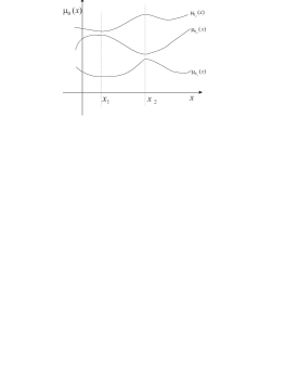
Figure 2: The best arm at time $t$ never depends on the side observation $X_{t}$. That is, for any possible pair, $(\theta_{1},\theta_{2})$, the two curves, $\mu_{\theta_{1}}(x)$ and $\mu_{\theta_{2}}(x)$, do not intersect each other. However, in this case, we can postpone our sampling to the most informative time instants.

The needed regularity conditions are similar to those in Section V:

1. ${\mathbf{X}}$ is a finite set and ${\mathsf{P}}_{G}(X_{t}=x)>0$ for all $x\in{\mathbf{X}}$.

2. $\forall\theta_{1},\theta_{2},x$, $I(\theta_{1},\theta_{2}|x)$ is strictly positive and finite.

In this case, one arm is always better than the other no matter what value of $X_{t}$ occurs. The conflict between learning and control still exists. As expected, the growth rate of the expected inferior sampling time is again lower bounded by $\log t$, but with the additional help of $X_{t}$ we can see improvements over the traditional bandit problems.

To greatly simplify the notation, we also assume that

1. For all $x$, the conditional expected reward $\mu_{\theta}(x)$ is strictly increasing w.r.t. $\theta$.

This condition gives us the notational convenience that the order of $(\mu_{\theta_{1}}(x),\mu_{\theta_{2}}(x))$ is simply the same as the order of $(\theta_{1},\theta_{2})$.

Example:

• ${\mathbf{\Theta}}=(1,\infty)$, ${\mathbf{X}}=\{1,2,3\}$, and the conditional reward distribution $F_{\theta}(\cdot|x)\sim{\mathcal{N}}(\theta x,1)$.

VI-B Lower Bound

Theorem 5 ($\log t$ Lower Bound)

Under the above assumptions, for any uniformly good rule $\{\phi_{\tau}\}$, $T_{inf}(t)$ satisfies

$$\lim_{t\rightarrow\infty}{\mathsf{P}}_{C_{0}}\left(T_{inf}(t)\geq\frac{(1-\epsilon)\log t}{K_{C_{0}}}\right)=1,~{}\forall\epsilon>0,$$

and $$\liminf_{t\rightarrow\infty}\frac{{\mathsf{E}}_{C_{0}}\{T_{inf}(t)\}}{\log t}\geq\frac{1}{K_{C_{0}}},$$ (2)

where $K_{C_{0}}$ is a constant depending on $C_{0}$. If $M_{C_{0}}=2$, then $T_{inf}(t)=T_{1}(t)$. The constant $K_{C_{0}}$ can be expressed as follows.

$$K_{C_{0}}=\inf_{\theta:\theta>\theta_{2}}\sup_{x\in{\mathbf{X}}}\{I(\theta_{1},\theta|x)\}.$$ (3)

The expression for $K_{C_{0}}$ for the case in which $M_{C_{0}}=1$ can be obtained by symmetry.

Note 1: if the decision maker is not able to access the side observation $X_{t}$, the player will then face the unconditional reward distribution $\int_{x}F_{\theta_{i}}(dy|x)G(dx)$ rather than $F_{\theta_{i}}(dy|x)$. Let $I(\theta_{1},\theta_{2})$ denote the Kullback-Leibler information between the unconditional reward distributions. By the convexity of the Kullback-Leibler information, we have

$$\sup_{x}I(\theta_{1},\theta|x)\geq\int_{x}I(\theta_{1},\theta|x)G(dx)\geq I(\theta_{1},\theta).$$

This shows that the new constant in front of $\log t$, in (3), is no larger than the corresponding constant in (1), and the additional side information $X_{t}$ generally improves the decision made in the bandit problem. As we would expect, Theorem 5 collapses to Theorem 1 when $|{\mathbf{X}}|=1$.

Note 2: This situation is like having several related bandit machines, whose reward distributions are all determined by the common configuration pair $(\theta_{1},\theta_{2})$. The information obtained from one machine is also applicable to the other machines. If arm 2 is always better than arm 1, we wish to sample arm 2 most of the time (the control part), and force sample arm 1 once in a while (the learning part). With the help of the side information $X_{t}$, we can postpone our forced sampling (learning) to the most informative machine $X_{t}=x$. As a result, the constant in the $\log t$ lower bound in Theorem 1 has been further reduced to this new $\frac{1}{K_{C_{0}}}$.

A detailed proof of Theorem 5 is provided in Appendix D.

VI-C Scheme Achieving the Lower Bound

Consider the additional conditions as follows.

1. $\mathbf{\Theta}$ is finite.

2. A saddle point for $K_{C_{0}}$ exists; that is, for all $\theta_{1}<\theta_{2}$,

   $$\inf_{\theta:\theta>\theta_{2}}\sup_{x}I(\theta_{1},\theta|x)=\sup_{x}\inf_{\theta:\theta>\theta_{2}}I(\theta_{1},\theta|x).$$

With the above conditions, we construct a $\log t$-lower-bound-achieving scheme $\{\phi_{\tau}\}$, which is inspired by [12]. The following terms and quantities are necessary in the expression of $\{\phi_{\tau}\}$.

• Denote $\hat{C}_{t}:=(\theta^{\alpha},\theta^{\beta})$. Instead of the traditional $(\hat{\theta}_{1},\hat{\theta}_{2})$ representation, we use $(\theta^{\alpha},\theta^{\beta})$. Based on this representation, we are able to derive the following useful notation:

  $$\theta^{\alpha\wedge\beta} := \min(\theta^{\alpha},\theta^{\beta})$$

  $$\alpha\wedge\beta := \arg\min(\theta^{\alpha},\theta^{\beta})$$

  $$\theta^{\alpha\vee\beta} := \max(\theta^{\alpha},\theta^{\beta})$$

  $$\alpha\vee\beta := \arg\max(\theta^{\alpha},\theta^{\beta}).$$

  For instance, if $\theta^{\alpha}<\theta^{\beta}$, $\mu_{\theta^{\alpha}}(x)=\mu_{\theta^{\alpha\wedge\beta}}(x)$; arm ${\alpha\wedge\beta}$ represents arm $1$; $Y_{t}^{\alpha\vee\beta}$ is the reward of arm 2; and $T_{inf}(t)=T_{\alpha\wedge\beta}(t)=T_{1}(t)$.

• Choose an $\epsilon$ such that $0<\epsilon<\frac{1}{2}\min\left\{\rho(F_{\theta}(\cdot|x),F_{\vartheta}(\cdot|x)):\forall x\in{\mathbf{X}},\theta\neq\vartheta\in{\mathbf{\Theta}}\right\}$, where $\rho$ is the Prohorov metric. The whole system is well-sampled if there exists a unique estimate $\hat{C}_{t}=(\theta^{\alpha},\theta^{\beta})$, such that the empirical measure $L_{i}^{x}(t)$ falls into the $\epsilon$-neighborhood of $F_{i(\hat{C}_{t})}(\cdot|x)$, for all $x\in{\mathbf{X}}$ and $i\in\{1,2\}$. That is

  $$\exists\hat{C}_{t},\mbox{ s.t.~{}}\rho\left(L_{i}^{x}(t),F_{i(\hat{C}_{t})}(\cdot|x)\right)<\epsilon,~{}~{}\forall x\in{\mathbf{X}},i\in\{1,2\}.$$

• For any estimate $\hat{C}_{t}=(\theta^{\alpha},\theta^{\beta})$, define the most informative bandit according to $\hat{C}_{t}$ as

  $$x^{*}(\hat{C}_{t}) := \arg\max_{x}\inf_{\theta:\theta>\theta^{\alpha\vee\beta}}I(\theta^{\alpha\wedge\beta},\theta,x),$$

  and $\Lambda_{t}(\hat{C}_{t},\theta)$ to be the conditional likelihood ratio between the seemingly inferior arm $\theta^{\alpha\wedge\beta}$ and the competing parameter $\theta$:

  $$\Lambda_{t}(\hat{C}_{t},\theta):=\prod_{m=1}^{T_{\alpha\wedge\beta}^{x^{*}}(t)}\frac{F_{\theta^{\alpha\wedge\beta}}\left(dY_{\tau_{x^{*}}(m)}^{\alpha\wedge\beta}|x^{*}(\hat{C}_{t})\right)}{F_{\theta}\left(dY_{\tau_{x^{*}}(m)}^{\alpha\wedge\beta}|x^{*}(\hat{C}_{t})\right)},$$

  where $\tau_{x^{*}}(m)$ denotes the time instant of the $m$-th pull of arm $\alpha\wedge\beta$ when the side observation $X_{\tau}=x^{*}(\hat{C}_{\tau})$.

• Set a total number of $|{\mathbf{X}}|+|{\mathbf{\Theta}}|^{2}+|{\mathbf{\Theta}}|^{3}$ counters, including $|{\mathbf{X}}|$ counters, named “ctr($x$)”; $|{\mathbf{\Theta}}|^{2}$ counters, named “ctr($\hat{C}$)” for all possible $\hat{C}\in{\mathbf{\Theta}}^{2}$; and $|{\mathbf{\Theta}}|^{3}$ counters, named “ctr($\hat{C},\theta$)” for all possible $\hat{C}$ and $\theta$. Initially, all counters are set to zero.

Algorithm 3 $\phi_{t+1}$, the decision at time $t+1$

1:  if there exists $i\in\{1,2\}$ and $x\in{\mathbf{X}}$ such that $T^{x}_{i}(t)=0$, then {Cond0}

2:     $\phi_{t+1}\leftarrow(t+1)\mbox{~{}mod~{}}2$.

3:  else if the whole system is not well-sampled or $\theta^{\alpha}=\theta^{\beta}$, then {Cond1}

4:     $\mbox{ctr($X_{t+1}$)}\leftarrow\mbox{ctr($X_{t+1}$)}+1$ and $\phi_{t+1}\leftarrow\mbox{ctr($X_{t+1}$)}\mbox{~{}mod~{}}2$.

5:  else if $\theta^{\alpha\vee\beta}=\bar{\theta}:=\max{\mathbf{\Theta}}$, then {Cond2}

6:     $\phi_{t+1}\leftarrow 1$ if it is $\theta^{\alpha}=\bar{\theta}$. Otherwise, $\phi_{t+1}\leftarrow 2$.

7:  else {Cond3}

8:     $\mbox{ctr($\hat{C}_{t}$)}\leftarrow\mbox{ctr($\hat{C}_{t}$)}+1$.

9:     if ctr($\hat{C}_{t}$) is odd, then {Cond3a}

10:        $\phi_{t+1}\leftarrow M_{\hat{C}_{t}}(X_{t+1})$.

11:     else {Cond3b}

12:        $\theta^{*}\leftarrow\arg\min\{\Lambda_{t}(\hat{C}_{t},\theta):\theta>\theta^{\alpha\vee\beta}\}$.

13:        if $X_{t+1}=x^{*}(\hat{C}_{t})$ then {Cond3b1}

14:           if $\Lambda_{t}(\hat{C}_{t},\theta^{*})\leq t(\log t)^{2}$, then {Cond3b1a}

15:              $\mbox{ctr($\hat{C}_{t},\theta^{*}$)}\leftarrow\mbox{ctr($\hat{C}_{t},\theta^{*}$)}+1$.

16:              if $\exists k\in{\mathbb{N}}\mbox{ s.t.~{}}\mbox{ctr($\hat{C}_{t},\theta^{*}$)}=k^{2}$, then {Cond3b1a1}

17:                 $\phi_{t+1}\leftarrow k\mbox{~{}mod~{}}2$.

18:              else {Cond3b1a2}

19:                 $\phi_{t+1}\leftarrow 3-M_{\hat{C}_{t}}(X_{t+1})$.

20:              end if

21:           else {Cond3b1b}

22:              $\phi_{t+1}\leftarrow M_{\hat{C}_{t}}(X_{t+1})$.

23:           end if

24:        else {Cond3b2}

25:           $\phi_{t+1}\leftarrow M_{\hat{C}_{t}}(X_{t+1})$.

26:        end if

27:     end if

28:  end if

Theorem 6 (Asymptotic Tightness)

With the above conditions, the scheme described in Algorithm 3 achieves the $\log t$ lower bound (2), so that this $\{\phi_{\tau}\}$ is uniformly good and asymptotically optimal.

A complete analysis is provided in Appendix E.

VII Mixed case

The main difference between Sections V and VI is that in one case, for all possible $C_{0}$, $X_{t}$ always changes the preference order, while in the other, for all possible $C_{0}$, $X_{t}$ never changes the order. A more general case is a mixture of these two. In this section, we consider this mixed case, which is the main result of this paper.

VII-A Formulation

Besides the assumption of constant $G$, in this section, we consider the case in which for some $C\in{\mathbf{\Theta}}^{2}$, $M_{C}(x)$ is not a function of $x$. For the remaining $C$, there exist $x_{1}$ and $x_{2}$ s.t. $M_{C}(x_{1})=1$ and $M_{C}(x_{2})=2$. For future reference, when the configuration pair $C_{0}$ satisfies the latter case, we say the configuration pair $C_{0}$ is implicitly revealing. Fig. 3 illustrates this situation.

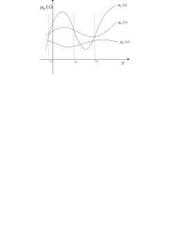
Figure 3: If $(\theta_{1},\theta_{2})=(\theta_{a},\theta_{b})$, the best arm depends on $x$, i.e. $\mu_{\theta_{1}}(x)$ and $\mu_{\theta_{2}}(x)$ intersect each other as in Section V. If $(\theta_{1},\theta_{2})=(\theta_{b},\theta_{c})$, the best arm does not depend on $x$, i.e. $\mu_{\theta_{1}}(x)$ and $\mu_{\theta_{2}}(x)$ do not intersect each other as in Section VI.

However, without knowledge of the authentic underlying configuration $C_{0}$, we do not know whether $C_{0}$ is implicitly revealing or not. In view of the results of Sections V and VI, we would like to find a single scheme that is able to achieve bounded ${\mathsf{E}}_{C_{0}}\{T_{inf}(t)\}$ when being applied to an implicitly revealing $C_{0}$, and on the other hand to achieve the $\log t$ lower bound when being applied to those $C_{0}$ which are not implicitly revealing.

The needed regularity conditions are the same as those in Sections V and VI:

1. ${\mathbf{X}}$ is a finite set and ${\mathsf{P}}_{G}(X_{t}=x)>0$ for all $x\in{\mathbf{X}}$.

2. $\forall\theta_{1},\theta_{2},x$, $I(\theta_{1},\theta_{2}|x)$ is strictly positive and finite.

To simplify the notation and the following proof, we define a partial ordering as $\theta\prec\vartheta$ iff $\forall x,\mu_{\theta}(x)\leq\mu_{\vartheta}(x)$, and $\theta\succ\vartheta$ is defined similarly. Note that for a configuration $C_{0}=(\theta_{1},\theta_{2})$, it can be the case that neither $\theta_{1}\prec\theta_{2}$ nor $\theta_{1}\succ\theta_{2}$.

Example:

• ${\mathbf{\Theta}}=(0,\infty)$, ${\mathbf{X}}=\{-1,1\}$ and the conditional reward distribution $F_{\theta}(\cdot|x)\sim{\mathcal{N}}(\theta^{2}-\theta x,1)$. Then $C_{0}=(\theta_{1},\theta_{2})=(0.1,0.2)$ is implicitly revealing, but $C_{0}=(0,10)$ is not.

VII-B Lower Bound

Theorem 7 ($\log t$ Lower Bound)

Under the above assumptions, for any uniformly good rule $\{\phi_{\tau}\}$, if $C_{0}$ is not implicitly revealing, $T_{inf}(t)$ satisfies

$$\lim_{t\rightarrow\infty}{\mathsf{P}}_{C_{0}}\left(T_{inf}(t)\geq\frac{(1-\epsilon)\log t}{K_{C_{0}}}\right)=1,~{}\forall\epsilon>0,$$

and $$\liminf_{t\rightarrow\infty}\frac{E_{C_{0}}\{T_{inf}(t)\}}{\log t}\geq\frac{1}{K_{C_{0}}},$$ (4)

where $K_{C_{0}}$ is a constant depending on $C_{0}$. If $M_{C_{0}}=2$, $T_{inf}(t)=T_{1}(t)$, and the constant $K_{C_{0}}$ can be expressed as follows.

$$K_{C_{0}}=\inf_{\left\{\theta:\exists x_{0},\mbox{ s.t.~{}}\mu_{\theta}(x_{0})>\mu_{\theta_{2}}(x_{0})\right\}}\sup_{x}\{I(\theta_{1},\theta|x)\}.$$

The expression for $K_{C_{0}}$ for the case in which $M_{C_{0}}=1$ can be obtained by symmetry.

The only difference between the lower bounds (2) and (4) is that, in (4), $K_{C_{0}}$ has been changed from taking the infimum over $\{\theta>\theta_{2}\}=\{\forall x,\mu_{\theta}(x)>\mu_{\theta_{2}}(x)\}$ to a larger set, $\{\theta:\exists x,\mu_{\theta}(x)>\mu_{\theta_{2}}(x)\}$. The reason for this is that under this case, consider a $\theta$ for which there exists $x$ such that $\mu_{\theta}(x)>\mu_{\theta_{2}}(x)$. If the authentic configuration is $C^{\prime}=(\theta,\theta_{2})$ rather than $(\theta_{1},\theta_{2})$, a linear order of incorrect sampling will be introduced, which violates the uniformly-good-rule assumption. As a result, a broader class of competing distributions $C^{\prime}=(\theta,\theta_{2})$ must be considered, i.e., we must consider a different set of configurations, over which the infimum is taken.

A detailed proof is contained in Appendix F.

VII-C Scheme Achieving the Lower Bound

Consider the same two additional conditions as those in Section VI.

1. $\mathbf{\Theta}$ is finite.

2. A saddle point for $K_{C_{0}}$ exists; that is, for all $\theta_{1}$,

   $$\inf_{\left\{\theta:\exists x_{0},\mu_{\theta}(x_{0})>\mu_{\theta_{2}}(x_{0})\right\}}\sup_{x}I(\theta_{1},\theta|x)$$

   $$=\sup_{x}\inf_{\left\{\theta:\exists x_{0},\mu_{\theta}(x_{0})>\mu_{\theta_{2}}(x_{0})\right\}}I(\theta_{1},\theta|x).$$

Algorithm 4 $\phi_{t+1}$, the decision at time $t+1$

1:  if there exists $i\in\{1,2\}$ and $x\in{\mathbf{X}}$ such that $T^{x}_{i}(t)=0$, then {Cond0}

2:     $\phi_{t+1}\leftarrow(t+1)\mbox{~{}mod~{}}2$.

3:  else if the whole system is not well-sampled or $\theta^{\alpha}=\theta^{\beta}$, then {Cond1}

4:     $\mbox{ctr($X_{t+1}$)}\leftarrow\mbox{ctr($X_{t+1}$)}+1$ and $\phi_{t+1}\leftarrow\mbox{ctr($X_{t+1}$)}\mbox{~{}mod~{}}2$.

5:  else if there exists $i\in\{1,2\}$, such that $\forall\theta,x,\mu_{\theta}(x)\leq\mu_{i(\hat{C}_{t})}(x)$, then {Cond2}

6:     $\phi_{t+1}\leftarrow i$, where $i$ is the satisfying index.

7:  else if $\hat{C}_{t}$ is implicitly revealing, then {Cond2.5}

8:     $\phi_{t+1}\leftarrow M_{\hat{C}_{t}}(X_{t+1})$.

9:  else {Cond3}

10:     $\mbox{ctr($\hat{C}_{t}$)}\leftarrow\mbox{ctr($\hat{C}_{t}$)}+1$.

11:     if ctr($\hat{C}_{t}$) is odd, then {Cond3a}

12:        $\phi_{t+1}\leftarrow M_{\hat{C}_{t}}(X_{t+1})$.

13:     else {Cond3b}

14:        $\theta^{*}\leftarrow\arg\min\{\Lambda_{t}(\hat{C}_{t},\theta):\forall\theta,\exists x_{0},\mbox{ s.t.~{}}\mu_{\theta}(x_{0})>\mu_{\theta^{\alpha\vee\beta}}(x_{0})\}$.

15:        if $X_{t+1}=x^{*}(\hat{C}_{t})$ then {Cond3b1}

16:           if $\Lambda_{t}(\hat{C}_{t},\theta^{*})\leq t(\log t)^{2}$, then {Cond3b1a}

17:              $\mbox{ctr($\hat{C}_{t},\theta^{*}$)}\leftarrow\mbox{ctr($\hat{C}_{t},\theta^{*}$)}+1$.

18:              if $\exists k\in{\mathbb{N}}\mbox{ s.t.~{}}\mbox{ctr($\hat{C}_{t},\theta^{*}$)}=k^{2}$, then {Cond3b1a1}

19:                 $\phi_{t+1}\leftarrow k\mbox{~{}mod~{}}2$.

20:              else {Cond3b1a2}

21:                 $\phi_{t+1}\leftarrow 3-M_{\hat{C}_{t}}(X_{t+1})$.

22:              end if

23:           else {Cond3b1b}

24:              $\phi_{t+1}\leftarrow M_{\hat{C}_{t}}(X_{t+1})$.

25:           end if

26:        else {Cond3b2}

27:           $\phi_{t+1}\leftarrow M_{\hat{C}_{t}}(X_{t+1})$.

28:        end if

29:     end if

30:  end if

A proposed scheme is described in Algorithm 4, which is similar to the scheme in Section VI-C. The only differences are the insertion of Cond2.5, Lines 7 and 8; the modification of Cond2, Lines 5 and 6; and the modification of Cond3b, line 14.

Notes:

1. When the estimate $\hat{C}_{t}=(\theta^{\alpha},\theta^{\beta})$ is not implicitly revealing, an ordering between $\theta^{\alpha}$ and $\theta^{\beta}$ exists. As a result, all notation regarding $\alpha\vee\beta$, $\theta^{\alpha\vee\beta}$, etc., remains valid.

2. The definition of $\Lambda_{t}(\hat{C}_{t},\theta)$ is slightly different. For any estimate $\hat{C}_{t}=(\theta^{\alpha},\theta^{\beta})$ that is not implicitly revealing, we can define the most informative bandit according to $\hat{C}_{t}$ as

   $$x^{*}(\hat{C}_{t})$$ (5)

   $$:=\arg\max_{x}\inf_{\{\theta:\exists x_{0},\mu_{\theta}(x_{0})>\mu_{\theta^{\alpha\vee\beta}}(x_{0})\}}I(\theta^{\alpha\wedge\beta},\theta|x),$$

   and $\Lambda_{t}(\hat{C}_{t},\theta)$ to be the conditional likelihood ratio between the seemingly inferior arm $\theta^{\alpha\wedge\beta}$ and the competing parameter $\theta$. That is,

   $$\Lambda_{t}(\hat{C}_{t},\theta):=\prod_{m=1}^{T_{\alpha\wedge\beta}^{x^{*}}(t)}\frac{F_{\theta^{\alpha\wedge\beta}}\left(\left.dY_{\tau_{x^{*}}(m)}^{\alpha\wedge\beta}\right|x^{*}(\hat{C}_{t})\right)}{F_{\theta}\left(\left.dY_{\tau_{x^{*}}(m)}^{\alpha\wedge\beta}\right|x^{*}(\hat{C}_{t})\right)},$$

   where $\tau_{x^{*}}(m)$ denotes the time instant of the $m$-th pull of arm $\alpha\wedge\beta$ when the side observation $X_{\tau}=x^{*}(\hat{C}_{\tau})$. (The difference between this new $\Lambda_{t}(\hat{C}_{t},\theta)$ and the previous one in Algorithm 3 is that we have a new $x^{*}(\hat{C}_{t})$ defined in (5).)

Theorem 8 (Asymptotic Tightness)

With the above conditions, the scheme described in Algorithm 4 has bounded $\lim_{t}{\mathsf{E}}_{C_{0}}\{T_{inf}(t)\}$, or achieves the $\log t$ lower bound (4), depending on whether the underlying configuration pair $C_{0}$ is implicitly revealing or not.

A detailed analysis is given in Appendix F.

VIII Conclusion

TABLE II: Summary of the Benefit of the Side Observations and the Required Regularity Conditions.

Characterization	Regularity Conditions	Results
$G_{C_{1}}\neq G_{C_{2}}$ iff $C_{1}\neq C_{2}$.	As $\hat{C}_{t}\rightarrow C_{0}$, $\forall x$, $M_{\hat{C}_{t}}(x)=M_{C_{0}}(x)$.	$\exists\{\phi_{\tau}\}$ s.t. $\forall C_{0}$, $\lim_{t}{\mathsf{E}}_{C_{0}}\{T_{inf}(t)\}<\infty$.
(i) Constant $G_{C}$, i.e., $G_{C}:=G$, (ii) $\forall C,\exists x_{1},x_{2}$, s.t. $M_{C}(x_{1})=1$, $M_{C}(x_{2})=2$ (implicitly revealing).	(i) $\mathbf{X}$ is finite. (ii) $\forall\theta_{1}\neq\theta_{2},x$, $0<I(\theta_{1},\theta_{2}|x)<\infty$. (iii) $\forall x$, $\mu_{\theta}(x)$ is continuous w.r.t. $\theta$.	$\exists\{\phi_{\tau}\}$ such that $\forall C_{0}$, $\lim_{t}{\mathsf{E}}_{C_{0}}\{T_{inf}(t)\}<\infty$.
(i) Constant $G_{C}$, i.e., $G_{C}:=G$, (ii) $\forall C$, $M_{C}(x)$ only depends on $C$, not on $x$.	(i) $\mathbf{X}$ is finite. (ii) $\forall\theta_{1}\neq\theta_{2},x$, $0<I(\theta_{1},\theta_{2}|x)<\infty$, (iii) $\forall x$, $\mu_{\theta}(x)$ is strictly increasing w.r.t. $\theta$.	For any uniformly good $\{\phi_{\tau}\}$, we have $\lim_{t}\frac{{\mathsf{E}}_{C_{0}}\{T_{inf}(t)\}}{\log t}\geq\frac{1}{K_{C_{0}}}$, $K_{C_{0}}:=\inf_{\theta}\sup_{x}I(\theta_{1},\theta|x)$. For finite $\mathbf{\Theta}$, $\exists\{\phi_{\tau}\}$, s.t. $\lim_{t}\frac{{\mathsf{E}}_{C_{0}}\{T_{inf}(t)\}}{\log t}\leq\frac{1}{K_{C_{0}}}$.
(i) Constant $G_{C}$, i.e., $G_{C}:=G$, (ii) The underlying $C_{0}$ may be implicitly revealing or not.	(i) $\mathbf{X}$ is finite. (ii) $\forall\theta_{1}\neq\theta_{2},x$, $0<I(\theta_{1},\theta_{2}|x)<\infty$.	For any uniformly good $\{\phi_{\tau}\}$, if $C_{0}$ is not implicitly revealing, we have $\lim_{t}\frac{{\mathsf{E}}_{C_{0}}\{T_{inf}(t)\}}{\log t}\geq\frac{1}{K_{C_{0}}}$, $K_{C_{0}}:=\inf_{\theta}\sup_{x}I(\theta_{1},\theta|x)$. For finite $\mathbf{\Theta}$, $\exists\{\phi_{t}\}$ s.t. (1) if $C_{0}$ is implicitly revealing, ${\mathsf{E}}_{C_{0}}\{T_{inf}(t)\}<\infty$, (2) if $C_{0}$ is not i.r., $\lim_{t}\frac{{\mathsf{E}}_{C_{0}}\{T_{inf}(t)\}}{\log t}\leq\frac{1}{K_{C_{0}}}$.

We have shown that observing additional side information can significantly improve sequential decisions in bandit problems. If the side observation itself directly provides information about the underlying configuration, then it resolves the dilemma of forced sampling and optimal control. The expected inferior sampling time will be bounded, as shown in Section IV. If the side observation does not provide information on the underlying configuration $(\theta_{1},\theta_{2})$, but always affects the preference order (implicitly revealing), then the myopic approach of sampling the seemingly-best arm will automatically sample both arms enough. The expected inferior sampling time is bounded, as shown in Section V. If the side observation does not affect the preference order at all, the dilemma still exists. However, by postponing our forced sampling to the most informative time instants, we can reduce the constant in the $\log t$ lower bound, as shown in Section VI. In Section VII, we combined the settings of Sections V and VI, and obtained a general result. When the underlying configuration $C_{0}$ is implicitly revealing (such that $X_{t}$ will change the preference order), we obtain bounded expected inferior sampling time as in Section V. Even if $C_{0}$ is not implicitly revealing (in that $X_{t}$ does not change the preference order), the new $\log t$ lower bound can be achieved as in Section VI. Our results are summarized in TABLE II.

Appendix A Sanov’s theorem and the Prohorov metric

For two distributions $P$ and $Q$ on the reals, the Prohorov metric is defined as follows.

Definition 2 (The Prohorov metric)

For any closed set $A\subset{\mathbb{R}}$ and $\epsilon>0$, define $A^{\epsilon}$, the $\epsilon$-flattening of $A$, as

$$A^{\epsilon}:=\left\{x\in{\mathbb{R}}:\inf_{y\in A}|x-y|<\epsilon\right\}.$$

The Prohorov metric $\rho$ is then defined as follows.

$$\rho(P,Q):=\inf\left\{\epsilon>0:P(A)\leq Q(A^{\epsilon})+\epsilon,\right.$$

$$\left.\mbox{ for all closed $A\subset{\mathbb{R}}$.}\right\}.$$

The Prohorov metric generates the topology corresponding to convergence in distribution. Throughout this paper, the open/closed sets on the space of distributions are thus defined accordingly.

Theorem 9 (Sanov’s theorem)

Let $L_{X}(n)$ denote the empirical measure of the real-valued i.i.d. random variables $X_{1},X_{2},\cdots,X_{n}$. Suppose $X_{i}$ is of distribution $P$ and consider any open set $A$ and closed set $B$ from the topological space of distributions, generated by the Prohorov metric. We have

$$\liminf_{n\rightarrow\infty}\frac{1}{n}\log{\mathsf{P}}_{P}(L_{X}(n)\in A) \geq -\inf_{Q\in A}I(Q,P)$$

$$\limsup_{n\rightarrow\infty}\frac{1}{n}\log{\mathsf{P}}_{P}(L_{X}(n)\in B) \leq -\inf_{Q\in B}I(Q,P).$$

Further discussion of the Prohorov metric and Sanov’s theorem can be found in [23, 24].

Appendix B Proof of Theorem 3

Proof:

For any underlying configuration pair $C_{0}=(\theta_{1},\theta_{2})$, define the error set ${\mathbf{C}}_{e}$ as follows.

$${\mathbf{C}}_{e} := \bigcup_{x\in{\mathbf{X}}}\{C\in{\mathbf{\Theta}}^{2}:M_{C}(x)\neq M_{C_{0}}(x)\}.$$ (6)

Let $\bar{{\mathbf{C}}}_{e}$ denote the closure of ${\mathbf{C}}_{e}$. By Condition 1, $C_{0}\notin\bar{{\mathbf{C}}}_{e}$. For any $t$, we can write

$${\mathsf{P}}_{C_{0}}\left(\phi_{t}\neq M_{C_{0}}(X_{t})\right) = {\mathsf{P}}_{C_{0}}\left(M_{\hat{C}_{t}}(X_{t})\neq M_{C_{0}}(X_{t})\right)$$

$$\leq {\mathsf{P}}_{C_{0}}\left(\exists x,M_{\hat{C}_{t}}(x)\neq M_{C_{0}}(x)\right)$$

$$= {\mathsf{P}}_{C_{0}}\left(\hat{C}_{t}\in{\mathbf{C}}_{e}\right)$$

$$\leq {\mathsf{P}}_{C_{0}}\left(\hat{C}_{t}\in\bar{{\mathbf{C}}}_{e}\right).$$

Let $\epsilon=\frac{1}{3}\inf\{\rho(G_{C_{0}},G_{C_{e}}):C_{e}\in\bar{{\mathbf{C}}}_{e}\}$, which is strictly positive by Condition 1, and consider sufficiently large $t\geq\frac{1}{\epsilon}$. If $\rho(G_{C_{0}},L_{X}(t))<\epsilon$, then by the definition of ${\mathbf{C}}_{t}$, $\rho(G_{\hat{C}_{t}},L_{X}(t))<\epsilon+\epsilon=2\epsilon$. By the triangle inequality, $\rho(G_{C_{0}},G_{\hat{C}_{t}})<3\epsilon$ and $\hat{C}_{t}\neq\bar{{\mathbf{C}}}_{e}$. As a result,

$$\{\hat{C}_{t}\in\bar{{\mathbf{C}}}_{e}\}\subset\left\{\rho(L_{X}(t),G_{C_{0}})\geq\epsilon\right\}\stackrel{{\scriptstyle\Delta}}{{=}}{\mathbf{K}}_{t}.$$

${\mathbf{K}}_{t}$ is a closed set. By Sanov’s theorem, the probability of ${\mathbf{K}}_{t}$ is exponentially upper bounded w.r.t. $t$, and so is ${\mathsf{P}}_{C_{0}}\left(\hat{C}_{t}\in\bar{{\mathbf{C}}}_{e}\right)$. As a result, we have

$$\lim_{t\rightarrow\infty}{\mathsf{E}}_{C_{0}}\{T_{inf}(t)\}=\lim_{t\rightarrow\infty}\sum_{\tau=1}^{t}{\mathsf{P}}_{C_{0}}(\phi_{\tau}\neq M_{C_{0}}(X_{\tau}))<\infty.$$

By the monotone convergence theorem, the expectation of $\lim_{t\rightarrow\infty}T_{inf}(t)$ is finite, which implies that $\lim_{t\rightarrow\infty}T_{inf}(t)$ is finite a.s. ∎

Appendix C Proof of Theorem 4

Similarly, we define ${\mathbf{C}}_{e}$ as that in (6). We need the following lemma to complete the analysis.

Lemma 1

With the regularity conditions specified in Section V, $\exists a_{1},a_{2}>0$ such that ${\mathsf{P}}_{C_{0}}(\hat{C}_{t}\in{\mathbf{C}}_{e})\leq a_{1}\exp\left(-a_{2}\min\left\{T_{1}^{x^{\star}}(t),T_{2}^{x^{\star}}(t)\right\}\right)$.

Proof of Lemma 1: By the continuity of $\mu_{\theta}(x)$ w.r.t. $\theta$ and the assumption of finite $\mathbf{X}$, it can be shown that $C_{0}\in\bar{\mathbf{C}}_{e}^{c}$. Therefore there exists a neighborhood of $C_{0}$, ${\mathbf{C}}_{\delta}=(\theta_{1}-\delta,\theta_{1}+\delta)\times(\theta_{2}-\delta,\theta_{2}+\delta)$, such that ${\mathbf{C}}_{\delta}\subset\bar{{\mathbf{C}}}_{e}^{c}\Leftrightarrow\bar{{\mathbf{C}}}_{e}\subset{\mathbf{C}}_{\delta}^{c}$.

Define a strictly positive $\epsilon>0$ as follows.

$$\epsilon:=\frac{1}{4}\inf\left\{\rho\left(F_{\hat{\theta}_{i}}(\cdot|x),F_{\theta_{i}}(\cdot|x)\right):~{}~{}~{}~{}~{}~{}~{}~{}~{}~{}~{}~{}~{}~{}~{}\right.$$

$$\left.\forall x\in{\mathbf{X}},i\in\{1,2\},(\hat{\theta}_{1},\hat{\theta}_{2})\in{\mathbf{C}}_{\delta}^{c}\right\}.$$

We would like to prove that for sufficiently large $t>\frac{1}{\epsilon}$,

$$\left\{\hat{C}_{t}\in{\mathbf{C}}_{\delta}^{c}\right\}\subset\left\{\exists i,\rho\left(L_{i}^{x^{\star}}(t),F_{\theta_{i}}(\cdot|x^{\star})\right)>\epsilon\right\}.$$

Suppose $\rho\left(L_{i}^{x^{\star}}(t),F_{\theta_{i}}(\cdot|x^{\star})\right)\leq\epsilon$ for both $i=1,2$. By the definition of $\sigma(C_{0},t)$, we have

$$\sigma(C_{0},t)\leq 2\epsilon.$$ (7)

However, for those $\hat{C}_{t}\in{\mathbf{C}}_{\delta}^{c}$, by the definition of $\epsilon$, for some $i\in\{1,2\}$, we have

$$\sigma(\hat{C}_{t},t) \geq \rho(F_{\hat{\theta}_{i}}(\cdot|x^{\star}),L_{i}^{x^{\star}}(t))$$ (8)

$$\geq \rho(F_{\hat{\theta}_{i}}(\cdot|x^{\star}),F_{\theta_{i}}(\cdot|x^{\star}))-\rho(F_{\theta_{i}}(\cdot|x^{\star}),L_{i}^{x^{\star}}(t))$$

$$\geq 3\epsilon,$$

which contradicts the definition of ${\mathbf{C}}_{t}$ since (7) and (8) imply $\sigma(\hat{C}_{t},t)>\frac{1}{t}+\sigma(C_{0},t)$. As a result, for sufficiently large $t$, we have

$$\left\{\hat{C}_{t}\in{\mathbf{C}}_{e}\right\} \subset \left\{\hat{C}_{t}\in{\mathbf{C}}_{\delta}^{c}\right\}$$ (9)

$$\subset \left\{\exists i,\rho\left(L_{i}^{x^{\star}}(t),F_{\theta_{i}}(\cdot|x^{\star})\right)>\epsilon\right\}$$

$$= \bigcup_{i=1,2}\left\{\rho\left(L_{i}^{x^{\star}}(t),F_{\theta_{i}}(\cdot|x^{\star})\right)>\epsilon\right\}.$$

By Sanov’s theorem, the probability of each term in the union of the right-hand side of (9) is exponentially bounded w.r.t. $T_{i}^{x^{\star}}(t)$. As a result, the probability of this finite union is bounded by $a_{1}\exp\left(-a_{2}\min\left\{T_{1}^{x^{\star}}(t),T_{2}^{x^{\star}}(t)\right\}\right)$ for some $a_{1}$, $a_{2}>0$.  ∎

Analysis of the scheme: We first use induction to show that $\forall t\geq 6$, $T_{i}(t)\geq\sqrt{t}$. This statement is true for $t=6$. Suppose $T_{t}(t-1)\geq\sqrt{t-1}$. If $T_{i}(t-1)\geq\sqrt{t}$, by the monotonicity of $T_{i}(t)$ w.r.t. $t$, we have $T_{i}(t)\geq T_{i}(t-1)\geq\sqrt{t}$. If $T_{i}(t-1)<\sqrt{t}$, by the forced sampling mechanism, $T_{i}(t)=T_{i}(t-1)+1\geq\sqrt{t-1}+1\geq\sqrt{t}$.

We consider the event of the inferior sampling at time $(t+1)$:

$$\left\{\phi_{t+1}\neq M_{C_{0}}(X_{t+1})\right\} = \left\{\phi_{t+1}\neq M_{C_{0}}(X_{t+1}),\hat{C}_{t}\in{\mathbf{C}}_{e}\right\}$$ (10)

$$~{}~{}\cup\left\{\phi_{t+1}\neq M_{C_{0}}(X_{t+1}),\hat{C}_{t}\in{\mathbf{C}}_{e}^{c}\right\}$$

$$\subset \left\{\hat{C}_{t}\in{\mathbf{C}}_{e}\right\}$$

$$~{}~{}\cup\left\{\phi_{t+1}\neq M_{C_{0}}(X_{t+1}),\hat{C}_{t}\in{\mathbf{C}}_{e}^{c}\right\}$$

$$\stackrel{{\scriptstyle\Delta}}{{=}} A_{t+1}\cup B_{t+1}.$$

Since $T_{i}(t)\geq\sqrt{t}$, we have $\min_{i}T_{i}(t)\geq\sqrt{t}$ and $\min_{i}T_{i}^{x^{\star}}(t)\geq\frac{\sqrt{t}}{|{\mathbf{X}}|}$. By Lemma 1, we have ${\mathsf{P}}_{C_{0}}(A_{t+1})\leq a_{1}e^{-a_{2}\frac{\sqrt{t}}{|{\mathbf{X}}|}}$, and hence $\sum^{\infty}_{t+1=7}{\mathsf{P}}_{C_{0}}(A_{t+1})<\infty$.

For ${\mathsf{P}}_{C_{0}}(B_{t+1})$, we can write

$$B_{t+1} = \left\{\phi_{t+1}\neq M_{\hat{C}_{t}}(X_{t+1}),\hat{C}_{t}\in{\mathbf{C}}_{e}^{c}\right\}$$ (11)

$$\subset \left\{\min\{T_{i}(t)\}_{i}<\sqrt{t+1},\hat{C}_{t}\in{\mathbf{C}}_{e}^{c}\right\}$$

$$= \left\{\min\{T_{i}(t)\}_{i}=\sqrt{t}\in{\mathbb{N}},\hat{C}_{t}\in{\mathbf{C}}_{e}^{c}\right\}$$

$$\subset \left\{\exists i,\phi_{a}\neq i,\forall a\in(\tau_{0},t],T_{i}(\tau_{0})=\sqrt{t}\right\}$$

$$\stackrel{{\scriptstyle\Delta}}{{=}} B_{t+1}^{1}\cup B_{t+1}^{2},$$

where $\tau_{0}=\left(\sqrt{t}-1\right)^{2}+1$ and $B_{t+1}^{1}$, $B_{t+1}^{2}$ correspond to $i=1,2$, respectively. The first equality comes from the fact that since $\hat{C}_{t}\in{\mathbf{C}}_{e}^{c}$, $M_{C_{0}}(X_{t+1})=M_{\hat{C}_{t}}(X_{t+1})$. The first subset sign comes from the fact that $\phi_{t+1}\neq M_{\hat{C}_{t}}(X_{t+1})$ implies the decision rule $\phi_{t+1}$ is in the stage of forced sampling. The second equality follows by combining both the inequalities: $\min\{T_{i}(t)\}_{i}\geq\sqrt{t}$ and $\min\{T_{i}(t)\}_{i}<\sqrt{t+1}$ and the fact that both $t$ and $T_{i}(t)$ are integers.

The reasoning behind the second subset inequality is as follows. By again using the fact that $T_{i}(t)\geq\sqrt{t}$ and substituting $\tau_{0}$ for $t$, we have $\sqrt{t}-1<T_{i}(\tau_{0})$ and thus have $T_{i}(\tau_{0})=\sqrt{t}=T_{i}(t)$, which guarantees that arm $i$ has not been sampled from time $\tau_{0}+1$ to $t$.

By the symmetry between $B_{t+1}^{1}$ and $B_{t+1}^{2}$, we can consider only $B_{t+1}^{1}$ for example. We have

$${\mathsf{P}}_{C_{0}}\left(B_{t+1}^{1}\right)$$

$$\leq~{}{\mathsf{P}}_{C_{0}}\left(M_{\hat{C}_{a-1}}(X_{a})=2,\forall a\in(\tau_{0},t]\right)$$

$$=\prod_{a\in(\tau_{0},t]}{\mathsf{P}}_{C_{0}}\left(\left.M_{\hat{C}_{a-1}}(X_{a})=2\right|M_{\hat{C}_{b-1}}(X_{b})=2,\forall b\in(\tau_{0},a)\right)$$

$$\leq~{}\left(1-\min_{x}\{{\mathsf{P}}_{G}(X_{t}=x)\}\right)^{t-\tau_{0}}.$$ (12)

The first inequality comes from the definition of $\{\phi_{\tau}\}$ which implies that if $T_{1}(\tau_{0})=T_{1}(t)\geq\sqrt{t}$, the forced sampling mechanism is not active during the time interval $(\tau_{0},t]$. So $\phi_{a}=2$ implies $M_{\hat{C}_{a-1}}(X_{a})=2$, $\forall a\in(\tau_{0},t]$. The second inequality comes from the assumption of i.i.d. $\{X_{\tau}\}$, which implies that $X_{a}$ is independent of $\hat{C}_{b}$ and $X_{b}$ for all $b<a$. Since at least one $x$ will make $M_{\hat{C}_{a-1}}(X_{a})=1$, each term in the product is then upper bounded by $1-\min_{x}\{{\mathsf{P}}_{G}(X_{t}=x)\}$. It is worth noting that by the regularity assumption on $G$, $1-\min_{x}\{{\mathsf{P}}_{G}(X_{t}=x)\}$ is strictly less than $1$.

Then from (11), (12), and the union bound, we obtain ${\mathsf{P}}_{C_{0}}(B_{t+1})\leq{\mathsf{P}}_{C_{0}}(B_{t+1}^{1})+{\mathsf{P}}_{C_{0}}(B_{t+1}^{2})\leq 2a^{t-((\sqrt{t}-1)^{2}+1)}$ for some $a<1$. Hence $\sum_{t+1=7}^{\infty}{\mathsf{P}}_{C_{0}}(B_{t+1})<\infty$. From (10), we conclude that

$$\lim_{t\rightarrow\infty}{\mathsf{E}}_{C_{0}}\left\{T_{inf}(t)\right\}$$

$$\leq~{}6+\sum_{\tau+1=7}^{\infty}({\mathsf{P}}_{C_{0}}(A_{\tau+1})+{\mathsf{P}}_{C_{0}}(B_{\tau+1}))<\infty,$$

which completes the proof.  ∎

Appendix D Proof of Theorem 5

Proof:

The proof is inspired by [14]. Without loss of generality, we assume $M_{C_{0}}=2$, which immediately implies $T_{inf}(t)=T_{1}(t)$. Fix a $\theta$ with $\mu_{\theta}>\mu_{\theta_{2}}$, and define $C^{\prime}=(\theta,\theta_{2})$. Let $\lambda(n)$ denote the log likelihood ratio between $\theta_{1}$ and $\theta$ based on the first $n$ observed rewards of arm 1. That is

$$\lambda(n):=\sum^{n}_{m=1}\log\left(\frac{F_{\theta_{1}}(dY^{1}_{\tau(m)}|X_{\tau(m)})}{F_{\theta}(dY^{1}_{\tau(m)}|X_{\tau(m)})}\right),$$

where $\tau(m)$ is a random variable corresponding to the time index of the $m$-th pull of arm 1.

By conditioning on the sequence $\{X_{\tau(m)}\}$, $\lambda(n)$ is a sum of independent r.v.’s. Let $K_{C^{\prime}}:=\sup_{x\in{\mathbf{X}}}\{I(\theta_{1},\theta|x)\}$, and suppose there exists $\delta>0$ such that

$$\limsup_{n\rightarrow\infty}\frac{\lambda(n)}{n}>K_{C^{\prime}}+\delta,$$

with positive probability. Then with positive probability, there exists an $x_{0}$ such that the average of the subsequence for which $X_{\tau(m)}=x_{0}$, will be larger than $K_{C^{\prime}}+\delta$. This, however, contradicts the strong law of large numbers since the subsequence is i.i.d. and with marginal expectation $I(\theta_{1},\theta|x_{0})$. Thus we obtain

$$\limsup_{n\rightarrow\infty}\frac{\lambda(n)}{n}\leq K_{C^{\prime}},~{}~{}{\mathsf{P}}_{C_{0}}-a.s.$$ (13)

The inequality (13) is equivalent to the statement that with probability one, there are finitely many $n$ such that $\lambda(n)>n(K_{C^{\prime}}+\delta)$ for some $\delta>0$. And since $K_{C^{\prime}}>0$, this in turn implies there are at most finitely manly $n$ such that $\max_{m\leq n}\lambda(m)>n(K_{C^{\prime}}+\delta)$. As a result, we have

$$\limsup_{n\rightarrow\infty}\frac{\max_{m\leq n}\lambda(m)}{n}\leq K_{C^{\prime}},~{}~{}P_{C_{0}}-a.s.,$$

$$\mbox{and~{}~{}~{}}\lim_{n\rightarrow\infty}{\mathsf{P}}_{C_{0}}\left(\exists m\leq n,\lambda(m)\geq(1+\delta)nK_{C^{\prime}}\right)=0.~{}~{}~{}$$ (14)

Henceforth, we proceed using contradiction. Suppose

$$\limsup_{t\rightarrow\infty}{\mathsf{P}}_{C_{0}}\left(T_{1}(t)<\frac{\log t}{(1+2\delta)K_{C^{\prime}}}\right)>0.$$

Using $A_{1}$ and $A_{2}$ as shorthand to denote events $A_{1}:=\left\{T_{1}(t)<\frac{\log t}{(1+2\delta)K_{C^{\prime}}}\right\}$ and $A_{2}:=\left\{\lambda(T_{1}(t))\leq\frac{(1+\delta)\log t}{(1+2\delta)}\right\}$, and by (14), we have

$$\limsup_{t\rightarrow\infty}{\mathsf{P}}_{C_{0}}\left(A_{1}\cap A_{2}\right)>0.$$ (15)

The quantity ${\mathsf{E}}_{C^{\prime}}\left\{T_{inf}(t)\right\}$ can be rewritten as follows.

$${\mathsf{E}}_{C^{\prime}}\left\{T_{inf}(t)\right\}$$

$$\stackrel{{\scriptstyle(a)}}{{=}}~{}{\mathsf{E}}_{C^{\prime}}\left\{T_{2}(t)\right\}$$

$$\stackrel{{\scriptstyle(b)}}{{=}}~{}{\mathsf{E}}_{C^{\prime}}\left\{t-T_{1}(t)\right\}$$

$$\stackrel{{\scriptstyle(c)}}{{\geq}}~{}\left(t-\frac{\log t}{(1+2\delta)K_{C^{\prime}}}\right){\mathsf{P}}_{C^{\prime}}\left(A_{1}\right)$$

$$\stackrel{{\scriptstyle(d)}}{{\geq}}~{}\left(t-\frac{\log t}{(1+2\delta)K_{C^{\prime}}}\right){\mathsf{P}}_{C^{\prime}}\left(A_{1}\cap A_{2}\right)$$

$$\stackrel{{\scriptstyle(e)}}{{\geq}}~{}\left(t-\frac{\log t}{(1+2\delta)K_{C^{\prime}}}\right)e^{-\frac{(1+\delta)\log t}{1+2\delta}}{\mathsf{P}}_{C_{0}}\left(A_{1}\cap A_{2}\right)$$

$$\stackrel{{\scriptstyle(f)}}{{=}}~{}{\mathcal{O}}\left(t^{\frac{\delta}{1+2\delta}}\right).$$ (16)

The equality marked $(a)$ follows from $M_{C^{\prime}}=1$ and $(b)$ follows from the fact that $T_{1}(t)+T_{2}(t)=t$. $(c)$ and $(d)$ follow from elementary probability inequalities. $(e)$ follows from the change-of-measure formula and the definition of $A_{2}$ in which $\lambda(T_{1}(t))\leq\frac{(1+\delta)\log t}{(1+2\delta)}$. $(f)$ follows from simple arithmetic and Eq. (15).

The inequality (16) contradicts the assumption that $\{\phi_{\tau}\}$ is uniformly good for both $C_{0}=(\theta_{1},\theta_{2})$ and $C^{\prime}=(\theta,\theta_{2})$, and thus we have

$$\lim_{t\rightarrow\infty}{\mathsf{P}}_{C_{0}}\left(T_{1}(t)\geq\frac{(1-\epsilon)\log t}{K_{C^{\prime}}}\right)=0,~{}~{}\forall\epsilon>0.$$

By choosing the $\theta$ in $C^{\prime}=(\theta,\theta_{2})$ with the minimizing configuration $\inf_{\theta>\theta_{2}}\sup_{x}I(\theta_{1},\theta|x)$, we complete the proof of the first statement of Theorem 5. The second statement in Theorem 5 can be obtained by simply applying Markov’s inequality and the first statement. ∎

Appendix E Proof of Theorem 6

We prove Theorem 6 by decomposing the inferior sampling time instants into disjoint subsequences, each of which will be discussed in separate lemmas respectively. For simplicity, throughout this proof, we use $1\{\mbox{\sf Cond1}(t)\}$ as shorthand for $1\{\mbox{\mbox{\sf Cond1} is satisfied at time $t$}\}$, and use $\delta\mbox{-nbd}(G)$ to denote the $\delta$-neighborhood of the distribution $G(x)$ on the $L^{\infty}$ space of distributions.

Suppose $M_{C_{0}}=2$. To prove that for the $\{\phi_{\tau}\}$ in Algorithm 3, $\limsup_{t\rightarrow\infty}\frac{{\mathsf{E}}_{C_{0}}T_{1}(t)}{\log t}\leq\frac{1}{\inf_{\theta>\theta_{2}}\max_{x}I(\theta_{1},\theta|x)}$, we first note the following:

$$T_{1}(t)$$ (17)

$$=~{}\sum_{\tau=1}^{t}1\{\phi_{\tau}=1\}$$

$$=~{}\sum_{\tau=1}^{t}1\{\phi_{\tau}=1,\mbox{\sf Cond0}(\tau)\}$$

$$~{}~{}~{}~{}+\sum_{\tau=1}^{t}1\{\phi_{\tau}=1,\mbox{\sf Cond1}(\tau)\}$$

$$~{}~{}~{}~{}+\sum_{\tau=1}^{t}1\{\phi_{\tau}=1,\mbox{\sf Cond2}(\tau)\}$$

$$~{}~{}~{}~{}+\sum_{\tau=1}^{t}1\{\phi_{\tau}=1,\hat{C}_{\tau-1}=(\theta^{\alpha},\theta^{\beta}),\theta^{\alpha}<\theta^{\beta}\neq\theta_{2},\mbox{\sf Cond3}(\tau)\}$$

$$~{}~{}~{}~{}+\sum_{\tau=1}^{t}1\{\phi_{\tau}=1,\hat{C}_{\tau-1}=(\theta^{\alpha},\theta^{\beta}),\theta_{1}\neq\theta^{\alpha}>\theta^{\beta},\mbox{\sf Cond3}(\tau)\}$$

$$~{}~{}~{}~{}+\sum_{\tau=1}^{t}1\{\phi_{\tau}=1,\hat{C}_{\tau-1}=(\theta^{\alpha},\theta^{\beta}),\theta_{1}\neq\theta^{\alpha}<\theta^{\beta}=\theta_{2},\mbox{\sf Cond3}(\tau)\}$$

$$~{}~{}~{}~{}+\sum_{\tau=1}^{t}1\{\phi_{\tau}=1,\hat{C}_{\tau-1}=(\theta^{\alpha},\theta^{\beta}),\theta_{1}=\theta^{\alpha}>\theta^{\beta},\mbox{\sf Cond3}(\tau)\}$$

$$~{}~{}~{}~{}+\sum_{\tau=1}^{t}1\{\phi_{\tau}=1,\hat{C}_{\tau-1}=(\theta^{\alpha},\theta^{\beta})=C_{0}=(\theta_{1},\theta_{2}),\mbox{\sf Cond3}(\tau)\}.$$

These eight terms of the right-hand side of (17) will be treated separately in Lemmas 2 through 8.

Lemma 2

Suppose $M_{C_{0}}=2$, i.e., $\theta_{1}<\theta_{2}$. Then

$$\forall C_{0}\in{\mathbf{\Theta}}^{2}, \lim_{t\rightarrow\infty}{\mathsf{E}}_{C_{0}}\left\{\sum_{\tau=1}^{t}1\{\phi_{\tau}=1,\mbox{\sf Cond0}(\tau)\}\right\}$$

$$\leq~{}\lim_{t\rightarrow\infty}{\mathsf{E}}_{C_{0}}\left\{\sum_{\tau=1}^{t}1\{\mbox{\sf Cond0}(\tau)\}\right\}<\infty.$$

Proof:

Let $T0:=\sum_{\tau=1}^{\infty}1\{\mbox{\sf Cond0}(\tau)\}$. By the monotone convergence theorem, it is equivalent to prove that ${\mathsf{E}}_{C_{0}}\left\{T0\right\}<\infty$ for all $C_{0}$. By the definition of Cond0, we have

$${\mathsf{P}}_{C_{0}}(T0=t)$$

$$\leq~{}\sum_{x\in{\mathbf{X}}}{\mathsf{P}}_{G}(X_{t}=x,\forall\tau<t\mbox{~{}and~{}}\tau\equiv t\mbox{~{}mod~{}}2,X_{\tau}\neq x)$$

$$=~{}\sum_{x\in{\mathbf{X}}}{\mathsf{P}}_{G}(X_{t}=x)(1-{\mathsf{P}}_{G}(X=x))^{[\frac{t-1}{2}]}$$

$$\leq~{}\left(1-\min_{x}{\mathsf{P}}_{G}(X_{t}=x)\right)^{[\frac{t-1}{2}]}.$$

By directly computing the expectation, we obtain ${\mathsf{E}}_{C_{0}}\{T0\}<\infty$. ∎

Lemma 3

Suppose $M_{C_{0}}=2$, i.e., $\theta_{1}<\theta_{2}$. Then

$$\lim_{t\rightarrow\infty}{\mathsf{E}}_{C_{0}}\left\{\sum_{\tau=1}^{t}1\{\phi_{\tau}=1,\mbox{\sf Cond1}(\tau)\}\right\}$$

$$\leq~{}\lim_{t\rightarrow\infty}{\mathsf{E}}_{C_{0}}\left\{\sum_{\tau=1}^{t}1\{\mbox{\sf Cond1}(\tau)\}\right\}<\infty.$$

Proof:

We define $L_{X}(t|\mbox{\sf Cond1})$ as the empirical distribution of $X_{\tau}$ at those time instants $\tau\leq t$ for which Cond1 is satisfied. We then have

$$\sum_{\tau=1}^{t}1\{\mbox{\sf Cond1}(\tau)\}$$

$$=~{}\sum_{\tau=1}^{t}1\{\mbox{\sf Cond1}(\tau),L_{X}(\tau|\mbox{\sf Cond1})\in\delta\mbox{-nbd}(G)\}$$

$$~{}~{}~{}~{}~{}+\sum_{\tau=1}^{t}1\{\mbox{\sf Cond1}(\tau),L_{X}(\tau|\mbox{\sf Cond1})\notin\delta\mbox{-nbd}(G)\}.$$ (18)

By Sanov’s theorem on finite alphabets (see [24]), each term in the second sum is exponentially upper bounded w.r.t. $\tau$, which implies the bounded expectation of the second sum. For the first sum, we have

$$\sum_{\tau=1}^{t}1\{\mbox{\sf Cond1}(\tau),L_{X}(\tau|\mbox{\sf Cond1})\in\delta\mbox{-nbd}(G)\}$$

$$\leq~{}\sum_{\tau=1}^{\infty}1\{\exists i,x,\mbox{ s.t.~{}}L_{i}^{x}(\tau-1)\notin\epsilon\mbox{-nbd}(F_{\theta_{i}}(\cdot|x)),$$

$$~{}~{}~{}~{}~{}~{}~{}~{}~{}~{}~{}~{}~{}~{}~{}~{}~{}~{}~{}\mbox{and }L_{X}(\tau|\mbox{\sf Cond1})\in\delta\mbox{-nbd}(G)\}$$

$$\leq~{}\sum_{x}\sum_{i=1}^{2}\sum_{\tau=1}^{\infty}1\{L_{i}^{x}(\tau-1)\notin\epsilon\mbox{-nbd}(F_{\theta_{i}}(\cdot|x)),$$

$$~{}~{}~{}~{}~{}~{}~{}~{}~{}~{}~{}~{}~{}~{}~{}~{}~{}~{}~{}~{}~{}~{}L_{X}(\tau|\mbox{\sf Cond1})\in\delta\mbox{-nbd}(G)\}$$ (19)

$$\leq~{}\sum_{x}\sum_{i=1}^{2}\sum_{\tau^{\prime}=1}^{\infty}1\{\exists n\geq\left[\frac{\tau^{\prime}{\mathsf{P}}_{G}(X=x)(1-\delta)-1}{2}\right],$$

$$~{}~{}~{}~{}~{}~{}~{}~{}~{}~{}~{}~{}~{}~{}~{}~{}~{}~{}~{}~{}~{}~{}~{}~{}\mbox{ s.t.~{}}\rho(L_{i}^{x}(n),F_{\theta_{i}}(\cdot|x))>\epsilon\}.$$ (20)

The first inequality comes from extending the finite sum to the infinite sum and the definition of Cond1. The second inequality comes from the union bound. The third inequality comes from the following three steps. First we change the summation index from the time variable $\tau$ to $\tau^{\prime}$, which specifies that it is the $\tau^{\prime}$-th time that the condition in (19) is satisfied. (Note: by definition, $\tau\geq\tau^{\prime}$.) Second, by $L_{X}(\tau|\mbox{\sf Cond1})\in\delta\mbox{-nbd}(G)$, there must be at least $\tau^{\prime}{\mathsf{P}}_{G}(X=x)(1-\delta)$ time instants that $X_{s}=x$, $s\leq\tau$, which guarantees we have enough access to the bandit machine $x$. And finally, by the definition of Cond1 in Algorithm 3, at the $\tau^{\prime}$-th time of satisfaction, the sample size $n$ must be greater than $\left[\frac{\tau^{\prime}{\mathsf{P}}_{C_{0}}(X=x)(1-\delta)-1}{2}\right]$. By slightly abusing the notation $L_{i}^{x}(t)$ with $L_{i}^{x}(n)$, where $n$ represents the sample size $T^{x}_{i}(t)$ rather than the current time $t$, we obtain the third inequality.

Remark: this change-of-index transformation will be used extensively throughout the proofs in this section.

By Sanov’s theorem on $\mathbb{R}$ (Theorem 9), the probability of each term in (20) is exponentially upper bounded w.r.t. $\tau^{\prime}$, which implies that the summation has bounded expectation. By (18), the proof of Lemma 3 is then complete. ∎

Lemma 4

Suppose $M_{C_{0}}=2$, i.e., $\theta_{1}<\theta_{2}$. Then

$$\lim_{t\rightarrow\infty}{\mathsf{E}}_{C_{0}}\left\{\sum_{\tau=1}^{t}1\{\phi_{\tau}=1,\mbox{\sf Cond2}(\tau)\}\right\}<\infty.$$

Proof:

By the assumption $\theta_{1}<\theta_{2}$, we have

$$\sum_{\tau=1}^{t}1\{\phi_{\tau}=1,\mbox{\sf Cond2}(\tau)\}$$

$$=~{}\sum_{\tau=1}^{t}1\{\hat{C}_{\tau-1}=(\theta^{\alpha},\theta^{\beta}),\theta^{\alpha}=\bar{\theta}\}$$

$$=~{}\sum_{\tau=1}^{t}1\{\hat{C}_{\tau-1}=(\theta^{\alpha},\theta^{\beta}),\theta^{\alpha}=\bar{\theta},L_{X}(\tau|\theta^{\alpha}=\bar{\theta})\in\delta\mbox{-nbd}(G)\}$$

$$~{}~{}~{}~{}+\sum_{\tau=1}^{t}1\{\hat{C}_{\tau-1}=(\theta^{\alpha},\theta^{\beta}),\theta^{\alpha}=\bar{\theta},L_{X}(\tau|\theta^{\alpha}=\bar{\theta})\notin\delta\mbox{-nbd}(G)\}$$

By Sanov’s theorem on finite alphabets, each term in the second sum is exponentially upper bounded w.r.t. $\tau$, which implies the bounded expectation of the second sum. For the first sum, we have

$$\sum_{\tau=1}^{t}1\{\hat{C}_{\tau-1}=(\theta^{\alpha},\theta^{\beta}),\theta^{\alpha}=\bar{\theta},L_{X}(\tau|\theta^{\alpha}=\bar{\theta})\in\delta\mbox{-nbd}(G)\}$$

$$\leq~{}\sum_{\tau=1}^{\infty}1\{\hat{C}_{\tau-1}=(\theta^{\alpha},\theta^{\beta}),\theta^{\alpha}=\bar{\theta},\exists x,\mbox{ s.t.~{}}$$

$$~{}~{}~{}~{}~{}~{}~{}~{}~{}~{}~{}~{}~{}~{}\rho(L_{1}^{x}(\tau-1),F_{\theta_{1}}(\cdot|x))>\epsilon,L_{X}(\tau|\theta^{\alpha}=\bar{\theta})\in\delta\mbox{-nbd}(G)\}$$

$$\leq~{}\sum_{x}\sum_{\tau^{\prime}=1}^{\infty}1\{\exists n\geq\left[\tau^{\prime}{\mathsf{P}}_{G}(X=x)(1-\delta)-1\right],\mbox{ s.t.~{}}$$

$$~{}~{}~{}~{}~{}~{}~{}~{}~{}~{}~{}~{}~{}~{}~{}~{}~{}~{}~{}~{}~{}~{}~{}~{}~{}~{}~{}~{}~{}~{}~{}~{}~{}~{}\rho(L_{1}^{x}(n),F_{\theta_{1}}(\cdot|x))>\epsilon\}.$$

By extending the finite sum to the infinite sum, we obtain the first inequality. By the definition of Cond2 in Algorithm 3 and using exactly the same reasoning used in going from (19) to (20), we obtain the second inequality. By Sanov’s theorem, each term in the above sum is exponentially upper bounded w.r.t. $\tau^{\prime}$. Thus it follows that the expectation of the first sum is also finite, which completes the proof. ∎

Lemma 5

Suppose $M_{C_{0}}=2$, i.e., $\theta_{1}<\theta_{2}$. Then

$$\lim_{t\rightarrow\infty}{\mathsf{E}}_{C_{0}}\left\{\sum_{\tau=1}^{t}1\left\{\phi_{\tau}=1,\hat{C}_{\tau-1}=(\theta^{\alpha},\theta^{\beta}),\right.\right.$$

$$~{}~{}~{}~{}~{}~{}~{}~{}~{}~{}~{}~{}~{}~{}~{}~{}~{}~{}~{}\left.\left.\theta^{\alpha}<\theta^{\beta}\neq\theta_{2},\mbox{\sf Cond3}(\tau)\right\}\right\}$$

$$\leq~{}\lim_{t\rightarrow\infty}{\mathsf{E}}_{C_{0}}\left\{\sum_{\tau=1}^{t}1\left\{\hat{C}_{\tau-1}=(\theta^{\alpha},\theta^{\beta}),\right.\right.$$

$$~{}~{}~{}~{}~{}~{}~{}~{}~{}~{}~{}~{}~{}~{}~{}~{}~{}~{}~{}\left.\left.\theta^{\alpha}<\theta^{\beta}\neq\theta_{2},\mbox{\sf Cond3}(\tau)\right\}\right\}$$

$$<~{}\infty.$$

Proof:

We have

$$\sum_{\tau=1}^{t}1\left\{\hat{C}_{\tau-1}=(\theta^{\alpha},\theta^{\beta}),\theta^{\alpha}<\theta^{\beta}\neq\theta_{2},\mbox{\sf Cond3}(\tau)\right\}$$

$$=~{}\sum_{(\theta,\vartheta):\theta<\vartheta\neq\theta_{2}}\sum_{\tau=1}^{t}1\{\hat{C}_{\tau-1}=(\theta,\vartheta),\mbox{\sf Cond3}(\tau)\}$$

$$\leq~{}2\sum_{(\theta,\vartheta):\theta<\vartheta\neq\theta_{2}}\sum_{\tau=1}^{t}1\{\hat{C}_{\tau-1}=(\theta,\vartheta),\mbox{\sf Cond3a}(\tau)\}$$

$$=~{}2\sum_{(\theta,\vartheta):\theta<\vartheta\neq\theta_{2}}\sum_{x}\sum_{\tau=1}^{t}1\{X_{\tau}=x,\hat{C}_{\tau-1}=(\theta,\vartheta),\mbox{\sf Cond3a}(\tau)\}$$

$$\leq~{}2\sum_{(\theta,\vartheta):\theta<\vartheta\neq\theta_{2}}\sum_{x}\sum_{\tau=1}^{\infty}1\{\rho(L_{2}^{x}(\tau-1),F_{\theta_{2}}(\cdot|x))>\epsilon,\mbox{\sf Cond3a}(\tau)\}$$

$$\leq~{}2\sum_{(\theta,\vartheta):\theta<\vartheta\neq\theta_{2}}\sum_{x}\sum_{\tau^{\prime}=1}^{\infty}1\{\exists n\geq\left[\tau^{\prime}-1\right],\mbox{ s.t.~{}}$$

$$~{}~{}~{}~{}~{}~{}~{}~{}~{}~{}~{}~{}~{}~{}~{}~{}~{}~{}~{}~{}~{}~{}~{}~{}~{}~{}~{}~{}~{}~{}~{}~{}~{}~{}~{}~{}~{}~{}~{}~{}~{}~{}~{}~{}~{}~{}~{}~{}~{}~{}~{}~{}\rho(L_{2}^{x}(n),F_{\theta_{2}}(\cdot|x))>\epsilon\}.$$

The first equality follows from conditioning on the event that the exact value of the estimate $\hat{C}_{\tau-1}$ is some configuration pair $(\theta,\vartheta)$. The first inequality follows from the definition of Cond3a in Algorithm 3, where double the number of time instants with odd ctr($\hat{C}$) will be larger than the total number of times that Cond3 is satisfied. The second equality follows from conditioning on the value of $X_{\tau}$. The second inequality follows from the condition that the second coordinate of the estimate, $\vartheta\neq\theta_{2}$, and then extending the finite sum to the infinite sum. The third inequality follows from the definition of Cond3a and changing the time index to $\tau^{\prime}$, similarly to the reasoning in (19)–(20). By Sanov’s theorem, each term is exponentially upper bounded w.r.t. $\tau^{\prime}$, and thus the entire sum has bounded expectation. The proof is thus complete. ∎

Corollary 1

By the symmetry of $\{\phi_{\tau}\}$, we have

$$\lim_{t\rightarrow\infty}$$

$${\mathsf{E}}_{C_{0}}\left\{\sum_{\tau=1}^{t}1\left\{\phi_{\tau}=1,\hat{C}_{\tau-1}=(\theta^{\alpha},\theta^{\beta}),\theta_{1}\neq\theta^{\alpha}>\theta^{\beta},\mbox{\sf Cond3}(\tau)\right\}\right\}$$

$$<~{}\infty.$$

Lemma 6

Suppose $M_{C_{0}}=2$, i.e., $\theta_{1}<\theta_{2}$. Then

$$\lim_{t\rightarrow\infty}{\mathsf{E}}_{C_{0}}\left\{\sum_{\tau=1}^{t}1\left\{\phi_{\tau}=1,\hat{C}_{\tau-1}=(\theta^{\alpha},\theta^{\beta})\right.\right.,$$

$$~{}~{}~{}~{}~{}~{}~{}~{}~{}~{}~{}~{}~{}\left.\left.\theta_{1}\neq\theta^{\alpha}<\theta^{\beta}=\theta_{2},\mbox{\sf Cond3}(\tau)\right\}\right\}<\infty.$$

Proof:

We have

$$\sum_{\tau=1}^{t}1\left\{\phi_{\tau}=1,\hat{C}_{\tau-1}=(\theta^{\alpha},\theta^{\beta}),\theta_{1}\neq\theta^{\alpha}<\theta^{\beta}=\theta_{2},\mbox{\sf Cond3}(\tau)\right\}$$

$$=~{}\sum_{\theta:\theta_{1}\neq\theta<\theta_{2}}\sum_{\tau=1}^{t}1\{\phi_{\tau}=1,\hat{C}_{\tau-1}=(\theta,\theta_{2}),\mbox{\sf Cond3}(\tau)\}$$

$$=~{}\sum_{\theta:\theta_{1}\neq\theta<\theta_{2}}\sum_{\tau=1}^{t}(1\{\phi_{\tau}=1,\hat{C}_{\tau-1}=(\theta,\theta_{2}),\mbox{\sf Cond3b1a1}(\tau)\}$$

$$~{}~{}~{}~{}~{}~{}~{}~{}~{}~{}~{}~{}~{}~{}~{}~{}~{}+1\{\phi_{\tau}=1,\hat{C}_{\tau-1}=(\theta,\theta_{2}),\mbox{\sf Cond3b1a2}(\tau)\})$$

$$\leq~{}\sum_{\theta_{1}\neq\theta<\vartheta=\theta_{2}}\sum_{\theta^{\prime}:\theta^{\prime}>\theta_{2}}$$

$$~{}~{}~{}~{}(\sum_{\tau=1}^{\infty}1\{\phi_{\tau}=1,\hat{C}_{\tau-1}=(\theta,\theta_{2}),\theta^{*}=\theta^{\prime},\mbox{\sf Cond3b1a1}(\tau)\}$$

$$~{}~{}~{}~{}+\sum_{\tau=1}^{\infty}1\{\phi_{\tau}=1,\hat{C}_{\tau-1}=(\theta,\theta_{2}),\theta^{*}=\theta^{\prime},\mbox{\sf Cond3b1a2}(\tau)\})$$ (21)

$$\leq~{}\sum_{\theta:\theta_{1}\neq\theta<\theta_{2}}\sum_{\theta^{\prime}:\theta^{\prime}>\theta_{2}}\sum_{\tau^{\prime}=1}^{\infty}$$

$$~{}~{}~{}~{}(4(\tau^{\prime}+1)^{2}-(2\tau^{\prime})^{2})\cdot 1\{\exists n\geq[\tau^{\prime}-1],\mbox{ s.t.~{}}$$

$$~{}~{}~{}~{}~{}~{}~{}~{}~{}~{}~{}~{}~{}~{}~{}~{}~{}~{}~{}~{}~{}~{}~{}~{}~{}~{}~{}~{}~{}~{}~{}~{}\rho(L_{1}^{x^{*}(\theta^{\prime})}(n),F_{\theta_{1}}(\cdot|x^{*}(\theta^{\prime})))>\epsilon\}.$$ (22)

The second equality comes from the fact that the scheme samples the inferior arm only when either Cond3b1a1 or Cond3b1a2 is satisfied. For the first inequality, we condition on $\theta^{*}$ and extend to the infinite sum. For the last inequality, we change the time index to $\tau^{\prime}$, which specifies the $\tau^{\prime}$-th satisfaction of Cond3b1a1, so that we can upper bound the first sum of (21). The reason we have a multiplication factor $(4(\tau^{\prime}+1)^{2}-(2\tau^{\prime})^{2})$ in front of the indicator function is in order to upper bound the second sum of (21), concerning Cond3b1a2, simultaneously.

To obtain this result, we note that between the consecutive times $\tau^{\prime}$ and $\tau^{\prime}+1$, at which Cond3b1a1 is satisfied and arm 1 is pulled, the number of times that Cond3b1a2 is satisfied and arm 1 is pulled cannot exceed $(2(\tau^{\prime}+1))^{2}-(2\tau^{\prime})^{2}-1$, which is because of the algorithm involving ctr($\hat{C}_{t},\theta^{*}$) in Line 16. Multiplying the factor $(4(\tau^{\prime}+1)^{2}-(2\tau^{\prime})^{2})$, we simultaneously bound these two sums.

By Sanov’s theorem, the expectation of the indicator in (22) is exponentially upper bounded w.r.t. $\tau^{\prime}$. As a result, the entire sum will have bounded expectation, which in turn completes the proof. ∎

Lemma 7

Suppose $M_{C_{0}}=2$, i.e., $\theta_{1}<\theta_{2}$. Then

$$\lim_{t\rightarrow\infty}{\mathsf{E}}_{C_{0}}\left\{\sum_{\tau=1}^{t}1\left\{\phi_{\tau}=1,\hat{C}_{\tau-1}=(\theta^{\alpha},\theta^{\beta}),\right.\right.$$

$$\left.\left.\theta_{1}=\theta^{\alpha}>\theta^{\beta},\mbox{\sf Cond3}(\tau)\right\}\right\}<\infty.$$

Proof:

We have,

$$\sum_{\tau=1}^{t}1\left\{\phi_{\tau}=1,\hat{C}_{\tau-1}=(\theta^{\alpha},\theta^{\beta}),\theta_{1}=\theta^{\alpha}>\theta^{\beta},\mbox{\sf Cond3}(\tau)\right\}$$

$$=~{}\sum_{\vartheta:\theta_{1}>\vartheta}\sum_{\tau=1}^{t}1\{\phi_{\tau}=1,\hat{C}_{\tau-1}=(\theta_{1},\vartheta),\mbox{\sf Cond3}(\tau)\}$$

$$\leq~{}\sum_{\vartheta:\theta_{1}>\vartheta}\sum_{\tau=1}^{t}1\{\hat{C}_{\tau-1}=(\theta_{1},\vartheta),\mbox{\sf Cond3}(\tau)\}$$

$$\leq~{}\sum_{\vartheta:\theta_{1}>\vartheta}\left(2\sum_{\tau=1}^{t}1\{\hat{C}_{\tau-1}=(\theta_{1},\vartheta),\mbox{\sf Cond3b}(\tau)\}+1\right)$$

$$=~{}\#\{\vartheta\in{\mathbf{\Theta}}:\vartheta<\theta_{1}\}+\sum_{\vartheta:\theta_{1}>\vartheta}$$

$$~{}~{}~{}~{}\left(2\sum_{\theta^{\prime}:\theta^{\prime}>\theta_{1}}\sum_{\tau=1}^{t}1\{\hat{C}_{\tau-1}=(\theta_{1},\vartheta),\theta^{*}=\theta^{\prime},\mbox{\sf Cond3b}(\tau)\}\right)$$

$$=~{}\#\{\vartheta\in{\mathbf{\Theta}}:\vartheta<\theta_{1}\}$$

$$~{}~{}~{}~{}+2\sum_{\vartheta:\theta_{1}>\vartheta}\sum_{\theta^{\prime}:\theta^{\prime}>\theta_{1}}\sum_{\tau=1}^{t}$$

$$~{}~{}~{}~{}~{}~{}~{}~{}~{}~{}(1\{\hat{C}_{\tau-1}=(\theta_{1},\vartheta),\theta^{*}=\theta^{\prime},$$

$$~{}~{}~{}~{}~{}~{}~{}~{}~{}~{}~{}~{}~{}~{}~{}~{}~{}~{}~{}\mbox{\sf Cond3b}(\tau),L_{X}(\tau|\mbox{\sf Cond3b})\in\delta\mbox{-nbd}(G)\}$$

$$~{}~{}~{}~{}~{}~{}~{}~{}~{}~{}~{}~{}+1\{\hat{C}_{\tau-1}=(\theta_{1},\vartheta),\theta^{*}=\theta^{\prime},$$

$$~{}~{}~{}~{}~{}~{}~{}~{}~{}~{}~{}~{}~{}~{}~{}~{}~{}~{}~{}\mbox{\sf Cond3b}(\tau),L_{X}(\tau|\mbox{\sf Cond3b})\notin\delta\mbox{-nbd}(G)\}).$$ (23)

The first inequality follows from Line 11 in Algorithm 3, where Cond3b is satisfied once after two times of Cond3 satisfaction. The last two equalities come from conditioning on $\theta^{*}$ and $L_{X}(\tau|\mbox{\sf Cond3b})$. By Sanov’s theorem on finite alphabets, the terms of the second sum in (23) are exponentially upper bounded and the entire sum thus has bounded expectation. For the first sum, we have

$$\sum_{\tau=1}^{t}1\{\hat{C}_{\tau-1}=(\theta_{1},\vartheta),\theta^{*}=\theta^{\prime},$$

$$~{}~{}~{}~{}~{}~{}~{}~{}~{}~{}~{}~{}~{}\mbox{\sf Cond3b}(\tau),L_{X}(\tau|\mbox{\sf Cond3b})\in\delta\mbox{-nbd}(G)\}$$

$$\leq~{}\frac{1}{{\mathsf{P}}_{G}(X=x^{*}(\theta_{1},\vartheta))(1-\delta)}\cdot$$

$$~{}~{}~{}~{}~{}\sum_{\tau=1}^{t}1\{\hat{C}_{\tau-1}=(\theta_{1},\vartheta),\theta^{*}=\theta^{\prime},\mbox{\sf Cond3b1}(\tau)\}.$$

(24)

This inequality follows from the fact that once $L_{X}$ falls into the $\delta$-nbd($G$), the total number of time instants can be upper bounded by the number of instants when $X_{\tau}=x^{*}(\theta_{1},\vartheta)$, over ${\mathsf{P}}_{G}(X=x^{*}(\theta_{1},\vartheta))(1-\delta)$. To show

$$\lim_{t\rightarrow\infty}{\mathsf{E}}_{C_{0}}\left\{\sum_{\tau=1}^{t}1\{\hat{C}_{\tau-1}=(\theta_{1},\vartheta),\theta^{*}=\theta^{\prime},\mbox{\sf Cond3b1}(\tau)\}\right\}<\infty,$$

we further decompose the expectand into

$$\sum_{\tau=1}^{t}1\{\hat{C}_{\tau-1}=(\theta_{1},\vartheta),\theta^{*}=\theta^{\prime},\mbox{\sf Cond3b1}(\tau)\}$$

$$=~{}\sum_{\tau=1}^{t}1\{\hat{C}_{\tau-1}=(\theta_{1},\vartheta),\theta^{*}=\theta^{\prime},\mbox{\sf Cond3b1a}(\tau)\}$$

$$~{}~{}~{}~{}+\sum_{\tau=1}^{t}1\{\hat{C}_{\tau-1}=(\theta_{1},\vartheta),\theta^{*}=\theta^{\prime},\mbox{\sf Cond3b1b}(\tau)\}.$$ (25)

For the first sum in (25), under the assumption $\theta_{1}>\vartheta$, we can write

$$\sum_{\tau=1}^{t}1\{\hat{C}_{\tau-1}=(\theta_{1},\vartheta),\theta^{*}=\theta^{\prime},\mbox{\sf Cond3b1a}(\tau)\}$$

$$\leq~{}\sum_{\tau=1}^{\infty}1\{\hat{C}_{\tau-1}=(\theta_{1},\vartheta),\theta^{*}=\theta^{\prime},\mbox{\sf Cond3b1a1}(\tau)\}$$

$$~{}~{}~{}~{}+\sum_{\tau=1}^{\infty}1\{\hat{C}_{\tau-1}=(\theta_{1},\vartheta),\theta^{*}=\theta^{\prime},\mbox{\sf Cond3b1a2}(\tau)\}$$

$$\leq~{}1+2\sum_{\tau=1}^{\infty}1\{\hat{C}_{\tau-1}=(\theta_{1},\vartheta),\theta^{*}=\theta^{\prime},\mbox{\sf Cond3b1a2}(\tau)\}$$

$$\leq~{}1+2\sum_{\tau^{\prime}=1}^{\infty}1\{\rho(\exists n\geq[\tau-1],\mbox{ s.t.~{}}$$

$$~{}~{}~{}~{}~{}~{}~{}~{}~{}~{}~{}~{}~{}~{}~{}~{}~{}~{}\rho(L_{2}^{x^{*}(\theta_{1},\vartheta)}(n),F_{\theta_{2}}(\cdot|x^{*}(\theta_{1},\vartheta)))>\epsilon\}.$$ (26)

The first inequality comes from conditioning on the sub-conditions Cond3b1a1 and Cond3b1a2, and extending to the infinite sums. Let ${\mathsf{SQ}}_{n}$ denote the set of perfectly squared integers in $\{1,\cdots,n\}$. The second inequality is from the definition of Cond3b1a1 in Algorithm 3 and the fact that $\forall n\in{\mathbb{N}}$, $|{\mathsf{SQ}}_{n}|$ is no larger than $1+|\{1,\cdots,n\}\backslash{\mathsf{SQ}}_{n}|$. The third inequality comes from the fact that by definition, under Cond3b1a2, $\phi_{\tau}=2$, and changing the time index to $\tau^{\prime}$, the number of satisfaction times. By Sanov’s theorem on $\mathbb{R}$, the above has bounded expectation.

For the second sum of (25), with the condition $\theta_{1}>\vartheta$

$$\sum_{\tau=1}^{t}1\{\hat{C}_{\tau-1}=(\theta_{1},\vartheta),\theta^{*}=\theta^{\prime},\mbox{\sf Cond3b1b}(\tau)\}$$

$$\leq~{}1+\sum_{\tau=1}^{t-1}1\{\hat{C}_{\tau}=(\theta_{1},\vartheta),\theta^{*}=\theta^{\prime},\Lambda_{\tau}(\hat{C}_{\tau},\theta^{\prime})>\tau(\log\tau)^{2}\}$$

$$\leq~{}1+\sum_{\tau=1}^{t-1}1\{\hat{C}_{\tau}=(\theta_{1},\vartheta),\Lambda_{\tau}(\hat{C}_{\tau},\theta_{2})>\tau(\log\tau)^{2}\}$$

$$\leq~{}1+\sum_{\tau=1}^{t-1}1\{\prod_{m=1}^{T_{2}^{x^{*}(\theta_{1},\vartheta)}(\tau)}\frac{F_{\vartheta}(dY_{\tau_{x^{*}}(m)}^{2}|x^{*}(\theta_{1},\vartheta))}{F_{\theta_{2}}(dY_{\tau_{x^{*}}(m)}^{2}|x^{*}(\theta_{1},\vartheta))}>\tau(\log\tau)^{2},\}$$

$$\leq~{}1+\sum_{\tau=1}^{t-1}1\{\exists n\leq\tau,\mbox{ s.t.~{}}\prod_{m=1}^{n}\frac{F_{\vartheta}(dY_{m|x^{*}}^{2}|x^{*}(\theta_{1},\vartheta))}{F_{\theta_{2}}(dY_{m|x^{*}}^{2}|x^{*}(\theta_{1},\vartheta))}>\tau(\log\tau)^{2}\},$$

where $Y^{2}_{m|x^{*}}$ is the reward of arm 2 at the $m$-th time that $X_{s}=x^{*}(\theta_{1},\vartheta)$ and $\phi_{s}=2$. The first inequality follows from focusing only on the $\Lambda_{\tau-1}(\hat{C}_{\tau-1},\theta^{\prime})$ condition in Cond3b1b and then shifting the time index $\tau$. The second inequality follows by replacing the minimum achieving $\theta^{\prime}$ with $\theta_{2}$. The third inequality follows from expressing $\Lambda_{\tau}$ using its definition. The fourth inequality follows from the set relationship, where $n$ is $T_{2}^{x^{*}(\theta_{1},\vartheta)}(\tau)$, the number of time instants that the side information $X_{s}=x^{*}(\theta_{1},\vartheta)$ and $\phi_{s}=2$, for $s\leq\tau$.

We first note that $\prod_{m=1}^{n}\frac{F_{\vartheta}(dY^{2}_{m|x^{*}}|x^{*}(\theta_{1},\vartheta))}{F_{\theta_{2}}(dY^{2}_{m|x^{*}}|x^{*}(\theta_{1},\vartheta))}$ is a positive martingale with expectation 1, when being considered under distribution $F_{\theta_{2}}(\cdot|x^{*}(\theta_{1},\vartheta))$. By Doob’s maximal inequality, we have

$${\mathsf{P}}_{C_{0}}\left(\exists n\leq\tau,\prod_{m=1}^{n}\frac{F_{\vartheta}(dY_{m|x^{*}}^{2}|x^{*}(\theta_{1},\vartheta))}{F_{\theta_{2}}(dY_{m|x^{*}}^{2}|x^{*}(\theta_{1},\vartheta))}>\tau(\log\tau)^{2}\right)\leq\frac{1}{\tau(\log\tau)^{2}},$$

and thus the expectation is bounded, i.e.,

$${\mathsf{E}}_{C_{0}}\left\{\sum_{\tau=1}^{t}1\{\hat{C}_{\tau-1}=(\theta_{1},\vartheta),\theta^{*}=\theta^{\prime},\mbox{\sf Cond3b1b}(\tau)\}\right\}$$

$$\leq~{}1+\sum_{\tau=1}^{\infty}\frac{1}{\tau(\log\tau)^{2}}<\infty.$$ (27)

By (23), (24), (25), (26), and (27), Lemma 7 is proved. ∎

Lemma 8

Suppose $M_{C_{0}}=2$, i.e., $\theta_{1}<\theta_{2}$. Then

$$\limsup_{t\rightarrow\infty}\frac{1}{\log t}\cdot$$

$${\mathsf{E}}_{C_{0}}\left\{\sum_{\tau=1}^{t}1\left\{\phi_{\tau}=1,\hat{C}_{\tau-1}=(\theta^{\alpha},\theta^{\beta})=(\theta_{1},\theta_{2}),\mbox{\sf Cond3}(\tau)\right\}\right\}$$

$$\leq~{}\frac{1}{\inf_{\theta>\theta_{2}}\max_{x}I(\theta_{1},\theta|x)}.$$

Proof:

By the definition of $\{\phi_{\tau}\}$, especially of Cond3b1a, we have

$${\mathsf{E}}_{C_{0}}\left\{\sum_{\tau=1}^{t}1\left\{\phi_{\tau}=1,\hat{C}_{\tau-1}=(\theta^{\alpha},\theta^{\beta})=C_{0}=(\theta_{1},\theta_{2}),\mbox{\sf Cond3}(\tau)\right\}\right\}$$

$$\leq~{}{\mathsf{E}}_{C_{0}}\left\{\sum_{\tau=1}^{t}1\{\hat{C}_{\tau-1}=C_{0},\mbox{\sf Cond3b1a}(\tau)\}\right\}$$

$$\leq~{}{\mathsf{E}}_{C_{0}}\left\{\sup\{1\leq n\leq t-1:\right.$$

$$~{}~{}~{}~{}~{}~{}~{}~{}~{}~{}~{}~{}~{}~{}~{}~{}\left.\min_{\theta>\theta_{2}}\prod_{m=1}^{n}\frac{F_{\theta_{1}}(dY_{m|x^{*}}^{1}|x^{*}(C_{0}))}{F_{\theta}(dY_{m|x^{*}}^{1}|x^{*}(C_{0}))}\leq t(\log t)^{2}\}\right\}$$

$$\leq~{}{\mathsf{E}}_{C_{0}}\left\{\sup\{1\leq n<\infty:\right.$$

$$~{}~{}~{}~{}~{}~{}~{}~{}~{}~{}~{}~{}~{}~{}~{}~{}\left.\min_{\theta>\theta_{2}}\prod_{m=1}^{n}\frac{F_{\theta_{1}}(dY_{m|x^{*}}^{1}|x^{*}(C_{0}))}{F_{\theta}(dY_{m|x^{*}}^{1}|x^{*}(C_{0}))}\leq t(\log t)^{2}\}\right\}$$

$$=~{}{\mathsf{E}}_{C_{0}}\left\{\max_{\theta>\theta_{2}}\sup\{1\leq n<\infty:\right.$$

$$~{}~{}~{}~{}~{}~{}~{}~{}~{}~{}~{}~{}~{}~{}~{}~{}\left.\prod_{m=1}^{n}\frac{F_{\theta_{1}}(dY_{m|x^{*}}^{1}|x^{*}(C_{0}))}{F_{\theta}(dY_{m|x^{*}}^{1}|x^{*}(C_{0}))}\leq t(\log t)^{2}\}\right\}$$

$$=~{}{\mathsf{E}}_{C_{0}}\left\{\max_{\theta>\theta_{2}}\sum_{s=1}^{\infty}1\{\inf_{n\geq s}\prod_{m=1}^{n}\frac{F_{\theta_{1}}(dY_{m|x^{*}}^{1}|x^{*}(C_{0}))}{F_{\theta}(dY_{m|x^{*}}^{1}|x^{*}(C_{0}))}\leq t(\log t)^{2}\}\right\},$$

where $Y^{1}_{m|x^{*}}$ denotes the reward of the $m$-th time that arm 1 of the sub-bandit machine $X_{\tau}=x^{*}(C_{0})$ is pulled. The first inequality follows because, by definition, only when Cond3b1a is satisfied can $\phi_{\tau}=1$, given $\hat{C}_{\tau-1}=C_{0}$. The second inequality is obtained by focusing on the sub-condition $\Lambda_{\tau}(\hat{C}_{\tau},\theta)$ in Cond3b1a, and letting $n=T_{1}^{x^{*}}(t-1)$ be the number of time instants when arm 1 is pulled and $X_{\tau}=x^{*}(C_{0})$. The third inequality comes from extending the upper bound of $n$ from $t-1$ to $\infty$. The equalities come from rearranging the $\max$ and $\min$ operators and elementary implications. By applying Lemma 4.3 of [12], quoted as Lemma 9 below, we have

$$\limsup_{t\rightarrow\infty}\frac{1}{\log t+2\log\log t}\cdot$$

$${\mathsf{E}}_{C_{0}}\left\{\max_{\theta>\theta_{2}}\sum_{s=1}^{\infty}1\{\inf_{n\geq s}\prod_{m=1}^{n}\frac{F_{\theta_{1}}(dY_{m|x^{*}}^{1}|x^{*}(C_{0}))}{F_{\theta}(dY_{m|x^{*}}^{1}|x^{*}(C_{0}))}\leq t(\log t)^{2}\}\right\}$$

$$\leq~{}\frac{1}{\min_{\theta>\theta_{2}}{\mathsf{E}}_{C_{0}}\left\{\log\left(\frac{F_{\theta_{1}}(dY_{m|x^{*}}^{1}|x^{*}(C_{0}))}{F_{\theta}(dY_{m|x^{*}}^{1}|x^{*}(C_{0}))}\right)\right\}}$$

$$=~{}\frac{1}{\min_{\theta>\theta_{2}}I(\theta_{1},\theta|x^{*}(C_{0}))}=\frac{1}{\max_{x}\inf_{\theta>\theta_{2}}I(\theta_{1},\theta|x)}$$

$$=~{}\frac{1}{\inf_{\theta>\theta_{2}}\max_{x}I(\theta_{1},\theta|x)},$$

where the equalities come from the existence-of-saddle-points assumption. By noting that $\log t\gg 2\log\log t$, this completes the proof of Lemma 8. ∎

By (17) and Lemmas 2 through 8, it has been proved that for the $\{\phi_{\tau}\}$ described in Algorithm 3,

$$\limsup_{t\rightarrow\infty}\frac{{\mathsf{E}}_{C_{0}}\left\{T_{inf}(t)\right\}}{\log t}\leq\frac{1}{K_{C_{0}}},~{}~{}\forall C_{0}\in{\mathbf{\Theta}}^{2}.$$

Lemma 4.3 of [12] is quoted as follows.

Lemma 9 (Lemma 4.3 of [12])

Suppose $Y_{1},Y_{2},\cdots$ are i.i.d. r.v.’s taking values in a finite set ${\mathbf{Y}}$, with marginal mass function $p(y)$. Let $f^{\theta}:{\mathbf{Y}}\rightarrow{\mathbb{R}}$ be such that $0<{\mathsf{E}}_{p}\{f^{\theta}(Y_{1})\}<\infty$, $\forall\theta\in\mathbf{\Theta}$, where $\mathbf{\Theta}$ is a finite set. Define $S^{\theta}_{t}=\sum_{\tau=1}^{t}f^{\theta}(Y_{\tau})$, $L^{\theta}_{A}=\sum_{\tau=1}^{\infty}1\{\inf_{t\geq\tau}S^{\theta}_{t}\leq A\}$, and $L_{A}=\max_{\theta\in\mathbf{\Theta}}L_{A}^{\theta}$. Then

$$\limsup_{A\rightarrow\infty}\frac{{\mathsf{E}}_{p}\{L_{A}\}}{A}\leq\frac{1}{\min_{\theta\in\mathbf{\Theta}}{\mathsf{E}}_{p}\{f^{\theta}(Y_{1})\}}.$$ (28)

Note: by incorporating Cramér’s theorem during the proof of this lemma in [12], it can be extended to continuous r.v.’s $Y_{1},Y_{2},\cdots$, provided ${\mathsf{E}}_{p}\left\{|f^{\theta}(Y_{1})|\right\}$ and ${\mathsf{E}}_{p}\left\{|f^{\theta}(Y_{1})|^{2}\right\}$ are finite for all $\theta$.

Appendix F Proof of Theorems 7 and 8

Proof of Theorem 7 ($\log t$ lower bound): This proof is basically a variation of that for Theorem 5, with the major difference being that the competing configuration $C^{\prime}=(\theta,\theta_{2})$ is now from a different set: $\{\theta:\exists x_{0},\mu_{\theta}(x_{0})>\mu_{\theta_{2}}(x_{0})\}$. We can first follow line by line in the proof of Theorem 5, and replace (16) with the following inequality.

$${\mathsf{E}}_{C^{\prime}}\left\{T_{inf}(t)\right\}$$

$$\geq~{}{\mathsf{E}}_{C^{\prime}}\left\{\sum_{\tau=1}^{t}1\{\phi_{\tau}=2,M_{C^{\prime}}(X_{\tau})=1\}\right\}$$

$$=~{}{\mathsf{E}}_{C^{\prime}}\left\{\sum_{\tau=1}^{t}1\{M_{C^{\prime}}(X_{\tau})=1\}-\right.$$

$$~{}~{}~{}~{}~{}~{}~{}~{}~{}~{}~{}~{}~{}~{}\left.\sum_{\tau=1}^{t}1\{\phi_{\tau}=1,M_{C^{\prime}}(X_{\tau})=1\}\right\}$$

$$\geq~{}{\mathsf{E}}_{C^{\prime}}\left\{\sum_{\tau=1}^{t}1\{M_{C^{\prime}}(X_{\tau})=1\}-\sum_{\tau=1}^{t}1\{\phi_{\tau}=1\}\right\}$$

$$\stackrel{{\scriptstyle(b)}}{{=}}~{}{\mathsf{E}}_{C^{\prime}}\left\{\pi t-T_{1}(t)\right\}$$

$$\stackrel{{\scriptstyle(c)}}{{\geq}}~{}\left(\pi t-\frac{\log t}{(1+2\delta)K_{C^{\prime}}}\right){\mathsf{P}}_{C^{\prime}}\left(A_{1}\right)$$

$$\stackrel{{\scriptstyle(d)}}{{\geq}}~{}\left(\pi t-\frac{\log t}{(1+2\delta)K_{C^{\prime}}}\right){\mathsf{P}}_{C^{\prime}}\left(A_{1}\cap A_{2}\right)$$

$$\stackrel{{\scriptstyle(e)}}{{\geq}}~{}\left(\pi t-\frac{\log t}{(1+2\delta)K_{C^{\prime}}}\right)e^{-\frac{(1+\delta)\log t}{1+2\delta}}{\mathsf{P}}_{C_{0}}\left(A_{1}\cap A_{2}\right)$$

$$\stackrel{{\scriptstyle(f)}}{{=}}~{}{\mathcal{O}}\left(t^{\frac{\delta}{1+2\delta}}\right),$$

where the first inequality comes from dropping the other half of the events where $\{\phi_{\tau}=1,M_{C^{\prime}}(X_{\tau})=2\}$. The second inequality comes from dropping the condition $M_{C^{\prime}}(X_{\tau})=1$. With $\pi:={\mathsf{P}}_{G}(M_{C^{\prime}}(X_{\tau})=1)>0$, recalling that $\theta^{\prime}$ satisfies that $\exists x_{0}$, such that $M_{C^{\prime}}(x_{0})=1$, we obtain $(b)$. $(c)$–$(f)$ follow from the same reasoning as discussed in connection with (16). From the contradiction of the uniformly-good-rule assumption, we have

$$\lim_{t\rightarrow\infty}{\mathsf{P}}_{C_{0}}\left(T_{1}(t)\geq\frac{(1-\epsilon)\log t}{K_{C^{\prime}}}\right)=0,~{}~{}\forall\epsilon>0.$$

By choosing the $\theta$ in $C^{\prime}=(\theta,\theta_{2})$ with the minimizing configuration $\inf_{\{\theta:\exists x,\mbox{ s.t.~{}}\mu_{\theta}(x)>\mu_{\theta_{2}}(x)\}}\sup_{x}I(\theta_{1},\theta|x)$, the proof of the first statement in Theorem 7 follows. The second statement in Theorem 7 can be obtained by simply applying Markov’s inequality and the first statement.  ∎

Proof of Theorem 8 (bound-achieving scheme): Following the same path as in the proof of Theorem 6, we first decompose the inferior sampling time instants into disjoint subsequences, each of which will be discussed separately.

$$T_{inf}(t)$$

$$=~{}\sum_{\tau=1}^{t}1\{\phi_{\tau}\neq M_{C_{0}}(X_{\tau})\}$$

$$=~{}\sum_{\tau=1}^{t}1\{\phi_{\tau}\neq M_{C_{0}}(X_{\tau}),\mbox{\sf Cond0}(\tau)\}$$

$$~{}~{}~{}~{}+\sum_{\tau=1}^{t}1\{\phi_{\tau}\neq M_{C_{0}}(X_{\tau}),\mbox{\sf Cond1}(\tau)\}$$

$$~{}~{}~{}~{}+\sum_{\tau=1}^{t}1\{\phi_{\tau}\neq M_{C_{0}}(X_{\tau}),\mbox{\sf Cond2}(\tau)\}$$

$$~{}~{}~{}~{}+\sum_{\tau=1}^{t}1\{\phi_{\tau}\neq M_{C_{0}}(X_{\tau}),\mbox{\sf Cond2.5}(\tau)\}$$

$$~{}~{}~{}~{}+\sum_{\tau=1}^{t}1\{\phi_{\tau}\neq M_{C_{0}}(X_{\tau}),\hat{C}_{\tau-1}=(\theta^{\alpha},\theta^{\beta}),$$

$$~{}~{}~{}~{}~{}~{}~{}~{}~{}~{}~{}~{}~{}~{}~{}\theta^{\alpha}\prec\theta^{\beta}\neq\theta_{2},\mbox{\sf Cond3}(\tau)\}$$

$$~{}~{}~{}~{}+\sum_{\tau=1}^{t}1\{\phi_{\tau}\neq M_{C_{0}}(X_{\tau}),\hat{C}_{\tau-1}=(\theta^{\alpha},\theta^{\beta}),$$

$$~{}~{}~{}~{}~{}~{}~{}~{}~{}~{}~{}~{}~{}~{}~{}\theta_{1}\neq\theta^{\alpha}\succ\theta^{\beta},\mbox{\sf Cond3}(\tau)\}$$

$$~{}~{}~{}~{}+\sum_{\tau=1}^{t}1\{\phi_{\tau}\neq M_{C_{0}}(X_{\tau}),\hat{C}_{\tau-1}=(\theta^{\alpha},\theta^{\beta}),$$

$$~{}~{}~{}~{}~{}~{}~{}~{}~{}~{}~{}~{}~{}~{}~{}\theta_{1}\neq\theta^{\alpha}\prec\theta^{\beta}=\theta_{2},\mbox{\sf Cond3}(\tau)\}$$

$$~{}~{}~{}~{}+\sum_{\tau=1}^{t}1\{\phi_{\tau}\neq M_{C_{0}}(X_{\tau}),\hat{C}_{\tau-1}=(\theta^{\alpha},\theta^{\beta}),$$

$$~{}~{}~{}~{}~{}~{}~{}~{}~{}~{}~{}~{}~{}~{}~{}\theta_{1}=\theta^{\alpha}\succ\theta^{\beta}\neq\theta_{2},\mbox{\sf Cond3}(\tau)\}$$

$$~{}~{}~{}~{}+\sum_{\tau=1}^{t}1\{\phi_{\tau}\neq M_{C_{0}}(X_{\tau}),\hat{C}_{\tau-1}=(\theta^{\alpha},\theta^{\beta})=C_{0}=(\theta_{1},\theta_{2}),$$

$$~{}~{}~{}~{}~{}~{}~{}~{}~{}~{}~{}~{}~{}~{}~{}\mbox{\sf Cond3}(\tau)\}.$$ (29)

By exactly the same analysis as in Lemmas 2 and 3, the first two sums in (29), concerning Cond0 and Cond1, have bounded expectations. Let $\bar{\theta}$ denote the configuration satisfying $\forall x_{0},\mu_{\theta}(x_{0})\leq\mu_{\bar{\theta}}(x_{0})$. For the sum concerning Cond2, $\{\phi_{\tau}\neq M_{C_{0}}(X_{\tau}),\mbox{\sf Cond2}(\tau)\}$ implies it is either $\theta^{\alpha}=\bar{\theta}\neq\theta_{1}$ or $\theta^{\beta}=\bar{\theta}\neq\theta_{2}$, where $(\theta^{\alpha},\theta^{\beta})=\hat{C}_{\tau-1}$. Both of the above cases are discussed in Lemma 4 and are proved to have finite expectations.

For future reference, we denote the five different sums concerning Cond3 as term3a, term3b, term3c, term3d, and term3e, in order. By Lemma 5 and Corollary 1, both term3a and term3b have bounded expectations.

If the underlying $C_{0}$ is not implicitly revealing, by Lemmas 6 and 7, term3c and term3d have bounded expectation. And by Lemma 8, $\limsup_{t}\frac{{\mathsf{E}}_{C_{0}}\{\mbox{\sf term3e}\}}{\log t}\leq K_{C_{0}}$.

If the underlying $C_{0}$ is implicitly revealing, $\mbox{\sf term3e}=0$. For term3c and term3d, we have

$$\sum_{\tau=1}^{t}1\{\phi_{\tau}\neq M_{C_{0}}(X_{\tau}),\hat{C}_{\tau-1}=(\theta^{\alpha},\theta^{\beta}),$$

$$~{}~{}~{}~{}~{}~{}~{}~{}~{}~{}\theta_{1}\neq\theta^{\alpha}\prec\theta^{\beta}=\theta_{2},\mbox{\sf Cond3}(\tau)\}$$

$$~{}~{}~{}+\sum_{\tau=1}^{t}1\{\phi_{\tau}\neq M_{C_{0}}(X_{\tau}),\hat{C}_{\tau-1}=(\theta^{\alpha},\theta^{\beta}),$$

$$~{}~{}~{}~{}~{}~{}~{}~{}~{}~{}~{}~{}~{}~{}~{}\theta_{1}=\theta^{\alpha}\succ\theta^{\beta}\neq\theta_{2},\mbox{\sf Cond3}(\tau)\}$$

$$\leq~{}\sum_{\tau=1}^{t}1\{\phi_{\tau}=1,\hat{C}_{\tau-1}=(\theta^{\alpha},\theta^{\beta}),\theta_{1}\neq\theta^{\alpha}\prec\theta^{\beta}=\theta_{2},\mbox{\sf Cond3}(\tau)\}$$

$$~{}~{}~{}+\sum_{\tau=1}^{t}1\{\phi_{\tau}=2,\hat{C}_{\tau-1}=(\theta^{\alpha},\theta^{\beta}),\theta_{1}\neq\theta^{\alpha}\prec\theta^{\beta}=\theta_{2},\mbox{\sf Cond3}(\tau)\}$$

$$~{}~{}~{}+\sum_{\tau=1}^{t}1\{\phi_{\tau}=1,\hat{C}_{\tau-1}=(\theta^{\alpha},\theta^{\beta}),\theta_{1}=\theta^{\alpha}\succ\theta^{\beta}\neq\theta_{2},\mbox{\sf Cond3}(\tau)\}$$

$$~{}~{}~{}+\sum_{\tau=1}^{t}1\{\phi_{\tau}=2,\hat{C}_{\tau-1}=(\theta^{\alpha},\theta^{\beta}),\theta_{1}=\theta^{\alpha}\succ\theta^{\beta}\neq\theta_{2},\mbox{\sf Cond3}(\tau)\},$$

(30)

which is obtained by replacing the condition $\phi_{\tau}\neq M_{C_{0}}(X_{\tau})$ with either $\phi_{\tau}=1$ or $\phi_{\tau}=2$. By Lemma 6, both the first and the fourth sums in (30) have bounded expectations. By Lemma 7, both the second and the third sums in (30) also have bounded expectations.

Note: in the proofs of Lemmas 6, 7, and 8, there are summations or minima taken on the set $\{\theta>\theta^{\beta}\}$. All those sets could be replaced by $\{\theta:\exists x_{0},\mbox{ s.t.~{}}\mu_{\theta}(x_{0})>\mu_{\theta^{\beta}}(x_{0})\}$ and the rest of the proofs still follow.

We have discussed all sub-sums in (29) except the sum regarding Cond2.5. It remains to show that the sum concerning Cond2.5 has bounded expectation, which is addressed in the following lemma.

Lemma 10

Consider the $\{\phi_{\tau}\}$ described in Algorithm 4. For all possible $C_{0}$, we have

$$\lim_{t\rightarrow\infty}{\mathsf{E}}_{C_{0}}\left\{\sum_{\tau=1}^{t}1\{\phi_{\tau}\neq M_{C_{0}}(X_{\tau}),\mbox{\sf Cond2.5}(\tau)\}\right\}<\infty.$$

Proof:

$$\sum_{\tau=1}^{t}1\{\phi_{\tau}\neq M_{C_{0}}(X_{\tau}),\mbox{\sf Cond2.5}(\tau)\}$$

$$\leq~{}\sum_{(\theta,\vartheta):(\theta,\vartheta)\neq C_{0}}\sum_{\tau=1}^{t}1\{\hat{C}_{\tau-1}=(\theta,\vartheta),\mbox{\sf Cond2.5}(\tau)\}$$

$$=~{}\sum_{(\theta,\vartheta):(\theta,\vartheta)\neq C_{0}}\sum_{\tau=1}^{t}1\{\hat{C}_{\tau-1}=(\theta,\vartheta),\mbox{\sf Cond2.5}(\tau),$$

$$~{}~{}~{}~{}~{}~{}~{}~{}~{}~{}~{}~{}~{}~{}~{}L_{X}(\tau|\mbox{\sf Cond2.5})\in\delta\mbox{-nbd}(G)\}$$

$$~{}~{}~{}~{}+\sum_{(\theta,\vartheta):(\theta,\vartheta)\neq C_{0}}\sum_{\tau=1}^{t}1\{\hat{C}_{\tau-1}=(\theta,\vartheta),\mbox{\sf Cond2.5}(\tau),$$

$$~{}~{}~{}~{}~{}~{}~{}~{}~{}~{}~{}~{}~{}~{}~{}L_{X}(\tau|\mbox{\sf Cond2.5})\notin\delta\mbox{-nbd}(G)\}$$ (31)

By Sanov’s theorem on finite alphabets, each term in the second sum is exponentially upper bounded w.r.t. $\tau$, which implies that the second sum has finite expectation. For the first sum, we have

$$\sum_{\tau=1}^{t}1\{\hat{C}_{\tau-1}=(\theta,\vartheta),\mbox{\sf Cond2.5}(\tau),$$ (32)

$$~{}~{}~{}~{}~{}~{}~{}~{}~{}~{}~{}~{}~{}~{}~{}L_{X}(\tau|\mbox{\sf Cond2.5})\in\delta\mbox{-nbd}(G)\}$$

$$\leq \sum_{\tau=1}^{t}1\{\hat{C}_{\tau-1}=(\theta,\vartheta),\theta\neq\theta_{1},\mbox{\sf Cond2.5}(\tau),$$

$$~{}~{}~{}~{}~{}~{}~{}~{}~{}~{}~{}~{}~{}~{}~{}L_{X}(\tau|\mbox{\sf Cond2.5})\in\delta\mbox{-nbd}(G)\}$$

$$+\sum_{\tau=1}^{t}1\{\hat{C}_{\tau-1}=(\theta,\vartheta),\vartheta\neq\theta_{2},\mbox{\sf Cond2.5}(\tau),$$

$$~{}~{}~{}~{}~{}~{}~{}~{}~{}~{}~{}~{}~{}~{}~{}L_{X}(\tau|\mbox{\sf Cond2.5})\in\delta\mbox{-nbd}(G)\},$$

which is obtained by considering whether $\theta\neq\theta_{1}$ or $\vartheta\neq\theta_{2}$, recalling that $(\theta,\vartheta)\neq C_{0}$. Since these two sums are symmetric, henceforth we show only the finite expectation of the first sum in (32). The finite expectation of the second sum then follows by symmetry.

$$\sum_{\tau=1}^{t}1\{\hat{C}_{\tau-1}=(\theta,\vartheta),\theta\neq\theta_{1},\mbox{\sf Cond2.5}(\tau),$$

$$~{}~{}~{}~{}~{}~{}~{}~{}~{}~{}~{}~{}~{}~{}~{}L_{X}(\tau|\mbox{\sf Cond2.5})\in\delta\mbox{-nbd}(G)\}$$

$$\leq~{}\sum_{\tau=1}^{t}1\{\exists x,\mbox{ s.t.~{}}M_{(\theta,\vartheta)}(x)=1,\rho(L_{1}^{x}(\tau-1),F_{\theta_{1}}(\cdot|x))>\epsilon,$$

$$~{}~{}~{}~{}~{}~{}~{}~{}~{}~{}~{}~{}\mbox{\sf Cond2.5}(\tau),L_{X}(\tau|\mbox{\sf Cond2.5})\in\delta\mbox{-nbd}(G)\}$$

$$\leq~{}\sum_{x:M_{(\theta,\vartheta)}(x)=1}\sum_{\tau^{\prime}=1}^{\infty}1\{\exists n\geq[\tau^{\prime}{\mathsf{P}}_{G}(X=x)(1-\delta)],\mbox{ s.t.~{}}$$

$$~{}~{}~{}~{}~{}~{}~{}~{}~{}~{}~{}~{}~{}~{}~{}\rho(L_{1}^{x}(n),F_{\theta_{1}}(\cdot|x))>\epsilon\}$$ (33)

The first inequality comes from the definition of Cond2.5: since $\hat{C}_{\tau-1}=(\theta,\vartheta)$ is implicitly revealing, there must be an $x$ s.t. $M_{\hat{C}_{\tau-1}}=1$. And since the estimate $\theta\neq\theta_{1}$, for that specific $x$, the distance between $L_{1}^{x}$ and $F_{\theta_{1}}(\cdot|x)$ must be greater than $\epsilon$. The second inequality comes from changing the time index to $\tau^{\prime}$, the time instants at which $X_{s}=x$ and Cond2.5 is satisfied, and extending the summation to infinity. (This change of the time index is similar to the one described in (19)–(20)).

Thus by Sanov’s theorem on $\mathbb{R}$, the expectation of each term in (33) is exponentially upper bounded w.r.t. $\tau^{\prime}$, which implies finite expectation of the entire sum in (33). By the discussions on (31), (32), and (33), Lemma 10 is proved. ∎

From the above discussion of the sub-sums in (29), we conclude that the modified scheme, $\{\phi_{\tau}\}$ in Algorithm 4, has bounded ${\mathsf{E}}_{C_{0}}\{T_{inf}(t)\}$ if the underlying $C_{0}$ is implicitly revealing. If $C_{0}$ is not implicitly revealing, the $\{\phi_{\tau}\}$ in Algorithm 4 achieves the new $\log t$ lower bound (4).  ∎

Chih-Chun Wang received the B.E. degree in electrical engineering from National Taiwan University, Taipei, Taiwan in 1999. He is currently working toward the Ph.D. degree in electrical engineering at Princeton University, Princeton, NJ. He worked in COMTREND Corporation, Taipei, Taiwan, from 1999-2000, and spent the summer of 2004 with Flarion Technologies. His research interests are in optimal control, information theory and coding theory, especially on iterative decoding of LDPC codes.

Sanjeev R. Kulkarni (M’91, SM’96, F’04) received the B.S. in Mathematics, B.S. in E.E., M.S. in Mathematics from Clarkson University in 1983, 1984, and 1985, respectively, the M.S. degree in E.E. from Stanford University in 1985, and the Ph.D. in E.E. from M.I.T. in 1991. From 1985 to 1991 he was a Member of the Technical Staff at M.I.T. Lincoln Laboratory working on the modeling and processing of laser radar measurements. In the spring of 1986, he was a part-time faculty at the University of Massachusetts, Boston. Since 1991, he has been with Princeton University where he is currently Associate Professor of Electrical Engineering and Associate Dean of Academic Affairs in the School of Engineering and Applied Science. He spent January 1996 as a research fellow at the Australian National University, 1998 with Susquehanna International Group, and summer 2001 with Flarion Technologies. Prof. Kulkarni received an ARO Young Investigator Award in 1992, an NSF Young Investigator Award in 1994, and several teaching awards at Princeton University. He has served as an Associate Editor for the IEEE Transactions on Information Theory. Prof. Kulkarni’s research interests include statistical pattern recognition, nonparametric estimation, learning and adaptive systems, information theory, wireless networks, and image/video processing.

H. Vincent Poor (S’72, M’77, SM’82, F’87) received the Ph.D. degree in EECS in 1977 from Princeton University, where he is currently the George Van Ness Lothrop Professor in Engineering. From 1977 until he joined the Princeton faculty in 1990, he was a faculty member at the University of Illinois at Urbana-Champaign. His research interests are primarily in the areas of stochastic analysis and statistical signal processing, with applications in wireless communications and related areas. Among his publications in this area is the recent book, Wireless Networks: Multiuser Detection in Cross-Layer Design. Dr. Poor is a member of the National Academy of Engineering, and is a Fellow of the Institute of Mathematical Statistics, the Optical Society of America, and other organizations. In 1990, he served as the President of the IEEE Information Theory Society and he is currently the Editor-in-Chief of the IEEE Transactions on Information Theory. Among his recent honors are the Joint Paper Award of the IEEE Communications and Information Theory Societies (2001), the NSF Director’s Award for Distinguished Teaching Scholars (2002), a Guggenheim Fellowship (2002-03), the IEEE EAB Major Educational Innovation Award (2004), and the IEEE Education Medal (2005).

References

- [1] H. Robbins, “Some aspects of the sequential design of experiments,” Bull. Am. Math. Soc., vol. 58, pp. 527–535, 1952.
- [2] K. Adam, “Learning while searching for the best alternative,” Journal of Economic Theory, vol. 101, pp. 252–280, 2001.
- [3] D. A. Berry, “A Bernoulli two-armed bandit,” Ann. Math. Stat., vol. 43, no. 3, pp. 871–897, June 1972.
- [4] H. Chernoff, Sequential Analysis and Optimal Design. Philadelphia: Society for Industrial and Applied Mathematics, 1972.
- [5] B. Ghosh and P.K.Sen, Handbook of Sequential Analysis. New York: Dekker, 1991.
- [6] J. C. Gittins, “Bandit processes and dynamic allocation indices,” J. Royal Statistical Society. Series B (Methodological), vol. 41, no. 2, pp. 148–177, 1979.
- [7] ——, “A dynamic allocation index for the discounted multiarmed bandit problem,” Biometrika, vol. 66, no. 3, pp. 561–565, Dec. 1979.
- [8] T. L. Lai and H. Robbins, “Asymptotically optimal allocation of treatments in sequential experiments,” in Design of Experiments : Ranking and Selection, Thomas J. Santner, Ajit C. Tamhane Eds. New York: Dekker, 1984.
- [9] ——, “Asymptotically efficient allocation rules,” Adv. Appl. Math., vol. 6, no. 1, pp. 4–22, 1985.
- [10] T. L. Lai and S. Yakowitz, “Machine learning and nonparametric bandit theory,” IEEE Trans. Automat. Contr., vol. 40, no. 7, pp. 1199–1209, July 1995.
- [11] R. Agrawal, M. V. Hegde, and D. Teneketzis, “Asymptotically efficient adaptive allocation rules for the multiarmed bandit problem with switching cost,” IEEE Trans. Automat. Contr., vol. 33, no. 10, pp. 899–906, Oct. 1988.
- [12] R. Agrawal, D. Teneketzis, and V. Anantharam, “Asymptotically efficient adaptive allocation schemes for controlled i.i.d. processes: Finite parameter space,” IEEE Trans. Automat. Contr., vol. 34, no. 3, pp. 258–267, Mar. 1989.
- [13] ——, “Asymptotically efficient adaptive allocation schemes for controlled Markov chains: Finite parameter space,” IEEE Trans. Automat. Contr., vol. 34, no. 12, pp. 1249–1259, Mar. 1989.
- [14] V. Anantharam, P. Varaiya, and J. Walrand, “Asymptotically efficient allocation rules for the multiarmed bandit problem with multiple plays-part I: I.i.d. rewards,” IEEE Trans. Automat. Contr., vol. 32, no. 11, pp. 968–976, Nov. 1987.
- [15] ——, “Asymptotically efficient allocation rules for the multiarmed bandit problem with multiple plays-part II: Markovian rewards,” IEEE Trans. Automat. Contr., vol. 32, no. 11, pp. 977–982, Nov. 1987.
- [16] M. N. Katehakis and H. Robbins, “Sequential choice from several populations,” in Proc. Nat. Acad. Sci. USA, vol. 92, Sept. 1995, pp. 8584–8585.
- [17] S. R. Kulkarni and G. Lugosi, “Finite-time lower bounds for the two-armed bandit problem,” IEEE Trans. Automat. Contr., vol. 45, no. 4, pp. 711–714, Apr. 2000.
- [18] M. K. Clayton, “Covariate models for Bernoulli bandits,” Sequential Analysis, vol. 8, no. 4, pp. 405–426, 1989.
- [19] S. R. Kulkarni, “On bandit problems with side observations and learnability,” in Proc. 31st Allerton Conf. Commun. Contr. Comp., Sept. 1993, pp. 83–92.
- [20] J. Sarkar, “One-armed bandit problems with covariates,” Ann. Statist., vol. 19, no. 4, pp. 1978–2002, 1991.
- [21] M. Woodroofe, “A one-armed bandit problem with a concomitant variable,” J. Amer. Stat. Assoc., vol. 74, no. 368, pp. 799–806, Dec 1979.
- [22] T. Zoubeidi, “Optimal allocations in sequential tests involving two populations with covariates,” Commun. Statist.: Theory and Methods, vol. 23, no. 4, pp. 1215–1225, 1994.
- [23] J. A. Bucklew, Large Deviation Techniques in Decision, Simulation, and Estimation. New York: Wiley, 1990.
- [24] A. Dembo and O. Zeitouni, Large Deviation Techniques and Applications. New York: Springer, 1998.