On The Tradeoff Between Two Types of Processing Gain

Abstract

One of the features characterizing almost every multiple access (MA) communication system is the processing gain. Through the use of spreading sequences, the processing gain of Random CDMA systems (RCDMA), or any other CDMA systems, is devoted to both bandwidth expansion and orthogonalization of the signals transmitted by different users. Another type of multiple access system is Impulse Radio (IR). IR systems promise to deliver high data rates over ultra wideband (UWB) channels with low complexity transmitters and receivers. In many aspects, IR systems are similar to time division multiple access (TDMA) systems, and the processing gain of IR systems represents the ratio between the actual transmission time and the total time between two consecutive transmissions (on-plus-off to on ratio). While CDMA systems, which constantly excite the channel, rely on spreading sequences to orthogonalize the signals transmitted by different users, IR systems transmit a series of short pulses and the orthogonalization between the signals transmitted by different users is achieved by the fact that most of the pulses do not collide with each other at the receiver.

In this paper, a general class of MA communication systems that use both types of processing gain is presented, and both IR and RCDMA systems are demonstrated to be two special cases of this more general class of systems. The bit error rate (BER) of several receivers as a function of the ratio between the two types of processing gain is analyzed and compared under the constraint that the total processing gain of the system is large and fixed. It is demonstrated that in non inter-symbol interference (ISI) channels there is no tradeoff between the two types of processing gain. However, in ISI channels a tradeoff between the two types of processing gain exists. In addition, the sub-optimality of RCDMA systems in frequency selective channels is established.

I Introduction

I-A Motivation

Multiple access (MA) communication systems are in widespread use. It is enough to mention that almost every cellular phone system and wireless local area network is an MA system. Many approaches for implementing multiple access systems exist; for example direct sequence code division multiple access (CDMA), frequency hopping, and time division, to name a few [8]. Recently, Impulse Radio (IR) systems have been suggested as a simple way of implementing MA systems [10]. Impulse Radio systems promise to deliver high data rates in multiple access channels with low complexity transmitters and receivers. Currently, IR systems are being considered for use in many applications and mainly as the preferred solution for communication systems transmitting over ultra wideband (UWB) channels [2, 3, 17, 18, 16, 19].

The two most popular ways for implementing MA systems are CDMA and time division multiple access (TDMA). These two types of systems are based on two different, and even “orthogonal” ideas. Consider a CDMA system and a TDMA system assigned with equal bandwidth and supporting identical users. In the CDMA system, each user’s transmitted signal’s bandwidth is expanded using a distinct spreading sequence, and all the users transmit simultaneously over the same channel. The purposes of the spreading sequences are to spread the transmitted energy over the assigned bandwidth and to make different users’ transmitted signals as close to orthogonal as possible. Alternatively, in a TDMA system, each user transmits for only a small fraction of the time but at a high data rate (and hence the need for large bandwidth). By preventing simultaneous transmissions from two different users, collisions between the signals transmitted by different users are avoided and hence the required rate from each user is achieved.

One type of CDMA systems are long-code CDMA systems, also known as random CDMA (RCDMA) systems [11, 13]. In RCDMA systems each user uses a random spreading sequence for expanding the bandwidth of the transmitted signal. Several MA communication systems are based on long-code CDMA, with the IS-95 mobile phone system being the most famous one [8]. As mentioned previously, IR systems have been suggested as a new approach to implementing MA communication systems. IR systems transmit a series of very short pulses, typically on the order of a fraction of a nano-second in duration. Each user transmits each pulse at a time slot randomly chosen, and each pulse is repeated several times. The receiver, using appropriate signal processing algorithms, recovers the transmitted bits [15]. IR systems can be regarded as random TDMA systems where each user transmits for a very short time at a time slot randomly chosen.

It is interesting to note that RCDMA systems and IR systems represent two extremes of a wide range of MA systems. In the first, the processing gain is devoted to increasing the signal bandwidth and making the different users’ transmitted signals as close to orthogonal as possible, while in the second the processing gain is mostly devoted to reducing the transmission time, which in turn reduces the probability of several users transmitting simultaneously. Although both IR and RCDMA systems have been analyzed in the past, the literature still lacks a study that examines the tradeoff between the types of processing gain represented by these two systems. Moreover, systems that use both types of processing gain have not been suggested and analyzed. This paper offers such a study by examining the performance of IR systems and the performance tradeoff between the two types of processing gain as a function of the system parameters for a fixed signaling environment.

The processing gain of IR systems, denoted hereafter by $N$, is $N=N_{f}N_{c}$. The pulse rate, $N_{f}$, represents the first type of processing gain, that is, the number of times each pulse is repeated (either uncoded or coded). Alternatively, $N_{c}$, which is the ratio between the average total time between two consecutive transmissions and the actual transmission time, is the second type of processing gain. Assume that the total processing gain is fixed. By changing the pulse rate, $N_{f}$, the ratio between the two types of processing gain is changed as well. The effect of this change on the system’s bit error rate (BER) is the main interest of this paper. Thus, throughout the rest of the paper we will compare systems that have equal total processing gain but which divide this total processing gain between the two types of processing gain differently.

I-B Signal Model

Consider the case of downlink channel of a $K$-user TH-IR synchronous cellular type system transmitting over a frequency-flat channel. Note that generalizing the results reported herein to more complex network configurations, e.g., uplink channels or asynchronous systems, can be easily carried out at the expense of complicating most of the, already complicated, computations, while the main results will essentially remain the same. The received signal, of say the $k$th user (out of $K$ total users in the system), in a binary phase-shift keyed random time hopping impulse radio (TH-IR) system can be described by the following continues time model,

$$r(t)=\sum_{k=1}^{K}\sqrt{\frac{E_{k}}{N_{f}}}\sum_{j=-\infty}^{\infty}d_{j}^{k}b_{\lfloor j/N_{f}\rfloor}^{k}w(t-jT_{f}-c_{j}^{k}T_{c})+n(t)$$ (1)

where $T_{f}$ is the average pulse repetition time, $w(t)$ is the transmitted unit-energy pulse, also referred to (in the UWB literature) as the monocycle, and $E_{k}$ is the transmitted energy per bit for user $k$. In order to allow the channel to be exploited by many users and to avoid catastrophic collisions, a long pseudo-random sequence $\{c_{j}^{k}\}$, such that $c_{j}^{k}$ is an integer taking one of the values in $[0,1,\ldots,N_{c}-1]$, is assigned to each user. Each sequence, usually referred to as the time hopping sequence, provides an additional time shift of $c_{j}^{k}T_{c}$ seconds to the $j$th pulse of the $k$th user. In order to avoid inter-pulse interference (IPI), it is usually required that $T_{c}\leq\frac{T_{f}}{N_{c}}$, so that overlaps between pulses originating from the same user are avoided. In typical IR systems each data symbol is transmitted over a set of multiple monocycles called a frame. Here $N_{f}$ denotes the number of pulses that correspond to one information symbol, i.e., the number of monocycles per frame. Thus, $b_{\lfloor j/N_{f}\rfloor}^{k}\in\{\pm 1\}$ is the information symbol transmitted during the $i=\lfloor j/N_{f}\rfloor$th frame. $n(t)$ represent white, Gaussian noise with power spectrum $\frac{N_{0}}{2}$ per hertz.

Two types of IR systems are considered in this paper. In the first type $d_{j}^{k}=1,\;\forall j,k$, while in the second the $d_{j}^{k}$’s are binary random variables, independent for $(i,k)\neq(j,l)$, taking each of the values $\pm 1$ with probability 1/2. The first type of system was the first to be proposed in the literature for transmission over UWB channels [7], while a different variant of the second was recently proposed in [9]. In the sequel, the two types of systems are referred to as uncoded and coded systems, respectively. Note that a coded IR systems can model an RCDMA system by taking $T_{f}=T_{c}$ and letting $N_{f}$ be the processing gain of the RCDMA system.

Denote by $\{s_{j}^{k}\}$ the following sequence

$$s_{j}^{k}=\left\{\begin{array}[]{cc}d_{\lfloor j/N_{c}\rfloor}^{k}&j-N_{f}\lfloor j/N_{c}\rfloor=c_{\lfloor j/Nc\rfloor}^{k}\\ 0&{\rm Otherwise}\\ \end{array}\right..$$ (4)

The sequence $\{s_{j}^{k}\}$ can be regarded as a pulse (or chip) rate spreading sequence where $s_{j}^{k}$ take the value $d_{\lfloor j/N_{c}\rfloor}^{k}$ whenever a pulse is transmitted and zero otherwise. Assuming, without loss of generality (wolog), that $\frac{T_{f}}{T_{c}}=N_{c}$, the received signal can be described by the following model,

$$r(t)=\sum_{k=1}^{K}\sqrt{\frac{E_{k}}{N_{f}}}\sum_{j=-\infty}^{\infty}s_{j}^{k}b_{\lfloor j/(N_{f}N_{c})\rfloor}^{k}w(t-jT_{c})+n(t).$$ (5)

Although (5) describes a continuous time TH-IR signal, discrete time equivalent models for CDMA systems can be used for describing the more general TH-IR systems. Assume that the received signal is passed through a linear filter matched to $w(t)$, and sampled at the pulse rate. Denote by ${\bf r}_{i}=[r_{iN_{f}N_{c}+1}\;\cdots\;r_{(i+1)N_{f}N_{c}}]^{T}$ the collection of all the samples corresponding to the $i$th frame. ${\bf r}_{i}$ can be described by the following linear model,

$${\bf r}_{i}={\bf S}_{i}{\bf A}{\bf b}_{i}+{\bf n}_{i}$$ (6)

where ${\bf S}_{i}=[{\bf s}_{i}^{1}\;\cdots{\bf s}_{i}^{K}]$ is the matrix whose columns are the spreading sequences used for spreading the $i$th information symbol of all the users, that is ${\bf s}_{i}^{k}\stackrel{{\scriptstyle\triangle}}{{=}}[s_{iN_{f}N_{c}+1}^{k}\;s_{iN_{f}N_{c}+2}^{k}\;\cdots\;s_{(i+1)N_{f}N_{c}}^{k}]^{T}$; ${\bf A}$ is a diagonal matrix with the users’ amplitudes on its diagonal, that is ${\bf A}=\frac{1}{\sqrt{N_{f}}}{\rm diag}[\sqrt{E_{1}}\;\cdots\;\sqrt{E_{K}}]$; ${\bf b}_{i}=[b_{i}^{1}\;\cdots b_{i}^{K}]^{T}$ is the vector containing the $i$th transmitted symbols of all the users; and ${\bf n}_{i}\sim{\mathcal{N}}\left(0,\sigma^{2}{\bf I}\right)$ is the additive noise. Note that a coded IR systems can model an RCDMA system by taking $N_{f}=N$ and letting $N_{f}$ be the processing gain of the RCDMA system. Also note that as $N_{f}$ decreases, the transmitted signal become more and more impulsive and hence the name Impulse Radio systems [6, 7, 9].

It is well known that ${\bf r}_{i}$ is a sufficient statistic for detecting the transmitted symbols. It is also well known that ${\bf y}_{i}={\bf S}_{i}^{T}{\bf r}_{i}$ is also a sufficient statistic for detecting the transmitted symbols. It is easily seen that ${\bf y}_{i}$ can be described by the following model,

$${\bf y}_{i}={\bf R}_{i}{\bf A}{\bf b}_{i}+\tilde{{\bf n}}_{i}$$ (7)

where ${\bf R}_{i}={\bf S}_{i}^{T}{\bf S}_{i}$ is the un-normalized cross-correlation matrix, with $N_{f}$ on its main diagonal and $\rho_{kl}^{i}=<{\bf s}_{i}^{k},{\bf s}_{i}^{l}>={\bf s}_{i}^{kT}{\bf s}_{i}^{l}=\sum_{j=1}^{N}[{\bf s}_{i}^{k}]_{j}[{\bf s}_{i}^{l}]_{j}$, as the off-diagonal elements; and where $\tilde{{\bf n}}_{i}$ is a zero mean, Gaussian random vector with correlation matrix $\sigma^{2}{\bf R}_{i}$.

Discrete time equivalent models for frequency selective channels are more complex. In order to have a tractable model that allows for analysis, we assume that a guard time equal to the length of the channel impulse response exists at the end of each symbol. This assumption is usually made in order to simplify the analysis [4]. As such, the following model for ${\bf r}_{i}$ is used in the sequel,

$${\bf r}_{i}={\bf H}_{0}{\bf S}_{i}{\bf A}{\bf b}_{i}+{\bf n}_{i}$$ (8)

where ${\bf H}_{0}$ is a lower-triangular Toeplitz matrix whose first column equals $[h_{0}\;h_{1}\;h_{2}\;\cdots\;h_{L}\;{\bf 0}]^{T}$.

I-C Organization of the Paper

The rest of the paper is organized as follows: In Section II, IR systems transmitting over frequency-flat channels are analyzed, and in Section III IR systems transmitting over frequency selective channels are analyzed. In Section IV some conclusions and concluding remarks are given. For convenience, numerical examples are presented at the end of each section.

II Transmission Over Flat Fading Channels

In this section, we focus on systems transmitting over flat fading channels. Both coded and uncoded systems are analyzed, and are shown to behave differently as a function of the pulse rate.

II-A Coded System

In this subsection coded-user systems are analyzed. The following simple lemma will be very useful in the analysis of both the matched filter detector and the optimal multiuser detector.

Lemma 1

Denote by ${\bm{\rho}}=[\rho_{1,2}\,\rho_{1,3}\,\ldots\,\rho_{K-1,K}]^{T}$, the vector containing cross-correlations between any two spreading sequences. Assume that $N\rightarrow\infty$ and that $\frac{N_{f}}{N_{c}}\rightarrow c>0$. Then ${\bm{\rho}}$ is asymptotically normally distributed with zero mean and correlation matrix $\frac{N_{f}}{N_{c}}{\bf I}$.

Proof of Lemma 1

See Appendix A

Consider the model for the received signal (7) scaled by $\frac{1}{\sqrt{N_{f}}}$,

$$\tilde{{\bf y}}_{i}=N_{f}^{-1/2}{\bf R}_{i}{\bf A}{\bf b}+N_{f}^{-1/2}{\bf n}.$$ (9)

According to Lemma 1, asymptotically (for large $N$) the vector of elements of $N_{f}^{-1/2}{\bf R}_{i}$ is distributed as a normal random vector with zero mean and correlation matrix $\frac{1}{N}{\bf I}$. Thus, for systems with large total processing gain, the distribution of $\tilde{{\bf y}}$, which is a sufficient statistic for detecting the transmitted symbols, is essentially independent of the pulse rate, and depends solely on $N$. Consequently the BER of any multiuser detection (MUD) algorithm which is based on ${\bf y}$ is essentially independent of the pulse rate. In particular the performance of the optimal, matched filter, minimum mean square error (MMSE), and zero forcing (ZF) multiuser detectors are independent of the pulse rate and depends solely on the total processing gain and not on the ratio between the two types of processing gains. Simulation results, which are not reported here due to space limitations, show that this result holds for systems with processing gains as low as $N=32$.

In the sequel we refer to a system satisfying $N_{f}<<N$ as a low pulse rate system, while a system such that $N_{f}$ is on the order of $N$ is referred to as a high pulse rate system. RCDMA is an example for a high pulse rate system since in this system $N_{f}=N$. It should be noted that as the pulse rate, $N_{f}$, decreases, the energy per transmitted pulse increases. This general behavior characterizes the main hardware complexity tradeoff between high pulse rate and low pulse rate systems. We demonstrate this hardware complexity by examining the matched filter (MF) detector.

The MF detector for detecting the $i$th symbol of the first user is $[{\bf y}_{i}]_{1}\stackrel{{\scriptstyle\textstyle>}}{{<}}_{b_{1}=-1}^{b_{1}=1}0$. Denote by $R_{s}$ the symbol rate. In order to implement the MF detector, the system sampling rate can be as low as $N_{f}R_{s}$, while the transmitted energy per pulse is $\frac{E}{N_{f}}$. These two terms represent a hardware complexity tradeoff between high and low pulse rate systems. While the sampling rate of low pulse rate systems can be lower than the sampling rate used by high pulse rate systems, the receiver dynamic range of low pulse rate systems must be higher than the receiver dynamic range of high pulse rate systems. The increase in the receiver dynamic range is due to the increase in the signal peak-to-average power ratio exhibited by low pulse rate systems.

II-B Uncoded System

In a way similar to the proof of Lemma 1 it is easy to verify that in uncoded-user systems ${\bm{\rho}}$ is asymptotically normally distributed with mean $\frac{N_{f}}{N_{c}}$ and covariance matrix $\frac{N_{f}}{N_{c}}\left(1-\frac{1}{N_{c}}\right){\bf I}$.

II-B1 Two User Systems

The Matched Filter Detector: Consider a two-uncoded-user system. For large N, the BER of the MF detector can be approximated as follows:

$$P_{e}=E_{\rho}(P_{e}|\rho)=E_{\rho}\left\{\frac{1}{2}Q\left(\frac{N_{f}\sqrt{\frac{E_{1}}{N_{f}}}-\sqrt{\frac{E_{2}}{N_{f}}}\rho}{\sigma\sqrt{N_{f}}}\right)\right.$$

$$+\left.\frac{1}{2}Q\left(\frac{N_{f}\sqrt{\frac{E_{1}}{N_{f}}}+\sqrt{\frac{E_{2}}{N_{f}}}\rho}{\sigma\sqrt{N_{f}}}\right)\right\}\cong$$

$$\frac{1}{2}Q\left(\frac{\sqrt{E_{1}}+\frac{\sqrt{E_{2}}}{N_{c}}}{\sqrt{\sigma^{2}+\frac{E_{2}}{N}\left(1-\frac{1}{N_{c}}\right)}}\right)+\frac{1}{2}Q\left(\frac{\sqrt{E_{1}}-\frac{\sqrt{E_{2}}}{N_{c}}}{\sqrt{\sigma^{2}+\frac{E_{2}}{N}\left(1-\frac{1}{N_{c}}\right)}}\right),$$ (10)

where $P_{e}|\rho$ is due to [12], and we used the identity ${\rm E}_{X}\left\{Q\left(\mu+\lambda X\right)\right\}=Q\left(\frac{\mu}{\sqrt{1+\lambda^{2}}}\right)$ for $X\sim{\mathcal{N}}\left(0,1\right)$.

It can be easily seen that asymptotically (as $N\rightarrow\infty$) the BER of the system depends on the ratio between the two types of processing gain, and hence there is a tradeoff between the two types of processing gains. The main question that arises is “what ratio between $N_{f}$ and $N_{c}$ minimizes the system BER?”. In Appendix B the following result is proven. Given that $\frac{E_{1}}{N}$ and $\frac{E_{2}}{N}$ are less than $\sigma^{2}$, and that $\frac{\sqrt{E_{2}}}{N}<\sqrt{E_{1}}<N\sqrt{E_{2}}$, the BER of (10) is a monotonically increasing function of the pulse rate. The above sufficient conditions means that the transmitted energy per chip is lower than the background noise level, and that the energies transmitted by the two users do not differ by a factor larger than the square of the processing gain. These conditions are almost always met in practical systems. Simulation results we conducted confirm that unless one of the users is much stronger than the other, low pulse rate systems are preferable over high pulse rate systems.

The superiority of low pulse rate systems over high pulse rate system can be intuitively deduced from (10) quite easily. Let us assume that $\frac{E_{2}}{N}<\frac{E_{1}}{N}<\sigma^{2}$. It can be easily seen that under this condition the approximate BER of the MF detector is the average of the $Q$ function over a simple random variable that can take one of two possible values. Due to our assumptions, on one hand, the average of these two values is approximately a constant independent of the pulse rate, and on the other as the pulse rate increases the distance between these two values increases as well. Since the $Q$ function is a convex function, Jensen’s inequality implies that the BER of the MF detector is a monotonically increasing function of the pulse rate.

Optimal Detector: In uncoded systems, it is quite clear from the asymptotic distribution of the correlation between the two users’ spreading sequences that the distribution of any sufficient statistic for detecting the transmitted symbols depends on the pulse rate. Thus, it is of interest to study the BER of the optimal MUD as a function of the pulse rate.

Denote by $P_{e}|\rho$ the probability of error of optimal MUD given that the correlation between the two users’ spreading sequences is $\rho$. It is well known that no general closed form expression for $P_{e}|\rho$ exists. Nevertheless, upper bounds for $P_{e}|\rho$ exist and it is easily seen that the one reported in [12] is a monotonically increasing function of $|\rho|$. As indicated by a large number of simulation studies, it is widely believed that $P_{e}|\rho$ is a monotonically increasing function of $|\rho|$ as well. Since in our system, $\rho$ is a random variable, the overall BER is given by averaging $P_{e}|\rho$ with respect to the distribution of $\rho$. Denote by $P_{e}|N_{f}$ this overall BER of optimal MUD given that the pulse rate equals $N_{f}$, i.e., $P_{e}|N_{f}={\rm E}_{\rho|N_{f}}\left\{P_{e}|\rho\right\}$.

Assume that $N_{f}<N_{f}^{\prime}$. Note that since the system is an uncoded one, $\rho|N_{f}\geq 0$ with probability one. In Appendix C it is proven that for all $x>0$ and large $N$, ${\textnormal{P}}\left((\rho|N_{f})<x\right)\geq{\textnormal{P}}((\rho|N_{f}^{\prime})<x)$. In the statistical literature this kind of relation between two random variables is usually termed first stochastic dominance and it is denoted as $\rho|N_{f}^{\prime}\succeq_{FSD}\rho|N_{f}$. It is well known that if $X\succeq_{FSD}Y$ and $U(\cdot)$ is a monotonically increasing function then ${\rm E}_{X}\left\{U(X)\right\}\geq{\rm E}_{Y}\left\{U(Y)\right\}$ [14]. Thus since $\rho|N_{f}^{\prime}\succeq_{FSD}\rho|N_{f}$ and the upper bound for the probability of error given $\rho$ is a monotonically increasing function of $\rho$, the average upper bound, which is also an upper bound for the average BER, is a monotonically increasing function of $N_{f}$ as well. By using the conjecture that the probability of error is a monotonically increasing function of $\rho$, and by using $\rho|N_{f}^{\prime}\succeq_{FSD}\rho|N_{f}$, we also conjecture that the BER of the optimal MUD is a monotonically increasing function of pulse rate.

II-B2 Multiple User Systems

In this section the BER of uncoded-user systems with arbitrary number of users using the matched filter detector or the optimal detector is examined. It is demonstrated that the general behavior observed for two-uncoded-user systems carries over to the case of a large number of users.

The matched filter detector for detecting the transmitted symbol, of say the first user, is, $[{\bf y}_{i}]_{1}=\sqrt{N_{f}E_{1}}b_{1}+\sum_{j=2}^{K}\sqrt{\frac{E_{j}}{N_{f}}}b_{j}\rho_{1,j}+[{\bf n}]_{1}\stackrel{{\scriptstyle\textstyle>}}{{<}}_{b_{1}=-1}^{b_{1}=1}0$, where $\rho_{1,j}$ is the $j$th element of the first row of ${\bf R}_{i}$. Assuming that $K$ is large, and all the users transmit with equal power, by invoking the Central Limit Theorem (CLT) $\frac{1}{\sqrt{K-1}}\sum_{j=1}^{K}\sqrt{\frac{E_{i}}{N_{f}}}b_{j}\rho_{1,j}$ is asymptotically normally distributed with zero mean and variance $\frac{E}{N_{f}}\left(\frac{N_{f}^{2}}{N_{c}^{2}}+\frac{N_{f}}{N_{c}}\left(1-\frac{1}{N_{c}}\right)\right)$. As a result, the BER of the MF detector can be approximated by

$$P_{e}\cong Q\left(\frac{\sqrt{E_{1}}}{\sqrt{\sigma^{2}+KE_{2}\left(\frac{1}{N}+\frac{1}{N_{c}^{2}}-\frac{1}{NN_{c}}\right)}}\right).$$ (11)

It is clear that the approximate system BER is a monotonically increasing function of the pulse rate as is the case for two user uncoded system. It is also clear that when the users transmit at different powers similar conclusion can be reached.

Analyzing the performance of the optimal multiuser detector is quite difficult due to the lack of closed-form expressions, or even simple upper bounds, for the system BER as a function of the users’ gains and correlation matrix. Nevertheless, we conjecture that, similarly to the case of a two-uncoded-user system, the system BER is a monotonically increasing function of the pulse rate. This conjecture is based on the observation that assuming $N_{f}<N_{f}^{\prime}$ then ${\bf R}_{i}|N_{f}\preceq_{FSD}{\bf R}_{i}|N_{f}^{\prime}$. That is, when the pulse rate decreases, the off-diagonal elements of ${\bf R}_{i}$ tends to be smaller, and hence the spreading sequences of the various users tends to be less correlated.

II-C Numerical Example

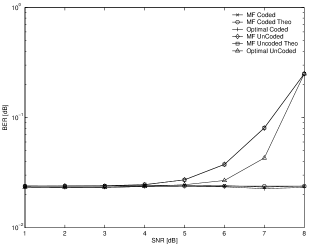
Figure 1: Probability of error as a function of the pulse rate. Two equal power users transmitting over a frequency-flat channel

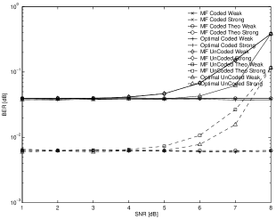
Figure 2: Probability of error as a function of the pulse rate. Two non-equal power users transmitting over a frequency-flat channel

In this subsection we present a numerical example that confirms the results reported thus far. We consider a system with processing gain $N=128$. Figures 1 and 2 depict the BER of both the MF detector and the optimal MUD as a function of the pulse rate. In Fig. 1 we assume two equal power users transmitting at signal to noise ratio (SNR) of 6dB, while in Fig. 2 we assume that the first user transmits at SNR of 5dB and the second use at SNR of 8dB. The theoretical expressions for the performance of the matched filter detector are depicted as well [6].

It is evident from the graph that the BERs of both the matched filter detector and the optimal multiuser detector in the coded system are unaffected by the pulse rate. Also the BERs of both the matched filter detector and the optimal multiuser detector in the uncoded system degrade considerably as the pulse rate increases. This is in accordance with the analysis conducted in this section. Moreover, we can see that the empirical and the theoretical curves agree well.

III Transmission over Frequency Selective channels

III-A Analysis

In this section, coded-user systems transmitting over frequency selective channels are analyzed. The analysis will be carried out in two stages. In the first stage it is assumed that only two paths arrive at the receiver, that is, the channel impulse response is ${\bf h}=[1\;{\bf 0}\;h_{l}]$, and that $l\leq N_{c}$. In the second step we will consider more general channels. Denote by $r_{j}$ the sample at the output of the matched filter at the time instant corresponding to the arrival time of the $j$th pulse from the user of interest, say the first user. The following model for $r_{j}$ can be easily deduced from (8),

$$r_{j}=\sqrt{\frac{E_{1}}{N_{f}}}d_{j}^{1}b_{1}+\sqrt{\frac{E_{1}}{N_{f}}}h_{l}d_{j-1}^{1}b_{1}I_{j}^{1}+\sqrt{\frac{E_{2}}{N_{f}}}d_{j}^{2}b_{2}I_{j}^{2}$$

$$+\sqrt{\frac{E_{2}}{N_{f}}}h_{l}d_{j-1}^{2}b_{2}I_{j}^{3}+n_{j}\quad,\quad j=1,\ldots,N_{f},$$ (12)

where $I_{j}^{1}$ is an indicator function taking the value one if the $(j-1)$th pulse transmitted by the first user collides via the second path with the $j$th pulse transmitted by the first user, and zero otherwise. $I_{j}^{2}$ is a function taking the value one if the $j$th pulse transmitted from the second user collides with the $j$th pulse transmitted from the first user, the value $h_{l}$ if the $j$th pulse transmitted from the second user and arriving via the second path collides with the $j$th pulse transmitted from the first user, and zero otherwise. $I_{j}^{3}$ is an indicator function taking the value one if the $(j-1)$th pulse transmitted by the second user collides via the second path with the $j$th pulse transmitted by the first user, and zero otherwise. The MF detector is

$$T=\sum_{j=1}^{N_{f}}d_{j}^{1}r_{j}=\sum_{j=1}^{N_{f}}\sqrt{\frac{E_{1}}{N_{f}}}b_{1}+\sqrt{\frac{E_{1}}{N_{f}}}h_{l}d_{j}^{1}d_{j-1}^{1}b_{1}I_{j}^{1}$$

$$+\sqrt{\frac{E_{2}}{N_{f}}}d_{j}^{1}d_{j}^{2}b_{2}I_{j}^{2}$$

$$+\sqrt{\frac{E_{2}}{N_{f}}}h_{l}d_{j}^{1}d_{j-1}^{2}b_{2}I_{j}^{3}+d_{j}^{1}n_{j}\stackrel{{\scriptstyle\textstyle>}}{{<}}_{b_{1}=-1}^{b_{1}=1}0.$$ (13)

In Appendix D it is shown that the multiple access interference (MAI), $\sum_{j=1}^{N_{f}}\sqrt{\frac{E_{1}}{N_{f}}}h_{l}d_{j}^{1}d_{j-1}^{1}b_{1}I_{j}^{1}+\sqrt{\frac{E_{2}}{N_{f}}}d_{j}^{1}d_{j}^{2}b_{2}I_{j}^{2}+\sqrt{\frac{E_{2}}{N_{f}}}h_{l}d_{j}^{1}d_{j-1}^{2}b_{2}I_{j}^{3}$, is asymptotically (as $N\rightarrow\infty$) normally distributed with zero mean and variance $E_{1}\frac{h_{l}^{2}l}{N_{c}^{2}}+E_{2}\frac{1+h_{l}^{2}}{N_{c}}$. Thus for systems with large processing gain, the distribution of the MF test statistic is approximately $T\sim{\mathcal{N}}\left(\sqrt{N_{f}E_{1}}b_{1},\frac{E_{1}h_{l}^{2}l}{N_{c}^{2}}+E_{2}\frac{1+h_{l}^{2}}{N_{c}}+N_{f}\sigma^{2}\right)$, and the BER can be approximated by,

$$P_{e}\cong Q\left(\frac{\sqrt{E_{1}}}{\sqrt{\sigma^{2}+E_{1}\frac{h_{l}^{2}l}{NN_{c}}+E_{2}\frac{1+h_{l}^{2}}{N}}}\right).$$ (14)

It can be easily seen from Appendix D that the multiple access interference is the sum of two independent terms. The first is the MAI created by the second user, $\sqrt{\frac{E_{2}}{N_{f}}}d_{j}^{1}d_{j}^{2}b_{2}I_{j}^{2}+\sqrt{\frac{E_{2}}{N_{f}}}h_{l}d_{j}^{1}d_{j-1}^{2}b_{2}I_{j}^{3}$, and the second is the self interference processes created by the first user upon itself, $\sum_{j=1}^{N_{f}}\sqrt{\frac{E_{1}}{N_{f}}}h_{l}d_{j}^{1}d_{j-1}^{1}b_{1}I_{j}^{1}$. Note that the self interference created by the first user is due to pulses arriving via the second path colliding with different pulses arriving via the first path; that is, this represents inter-pulse interference.

We now turn to the computation of the BER of the MF when more than two paths arrive at the receiver. The MAI created by the second user is asymptotically (as $N\rightarrow\infty$) normally distributed with zero mean and variance $E_{2}\frac{1+h_{l}^{2}}{N_{c}}$. This MAI can be modeled as the sum of two independent, zero mean Gaussian random variables, with variances $\frac{E_{2}}{N_{c}}$ and $\frac{E_{2}h_{l}^{2}}{N_{c}}$, respectively. The first (second) random variable represents the MAI caused by pulses originating from the second user and arriving at the receiver via the first (second) path. Hence, asymptotically, the MAI resulting from pulses arriving through different paths are independent. Using the same method used in Appendix D this can be generalized to channels with more than two paths or with two paths such that $l>N_{c}$. Thus, when the channel impulse response is arbitrary, the MAI created by the second user is asymptotically normally distributed with zero mean and variance $\frac{E_{2}}{N_{c}}\sum_{i=1}^{l}h_{i}^{2}=\frac{E_{2}||{\bf h}||}{N_{c}}$, which is the sum of the interference created by the different paths.

If the number of users in the system is larger than two it is easy to verify that the MAI processes due to different users are independent. Hence the total multiple access interference due to various users, is asymptotically (as $N\rightarrow\infty$) normally distributed with zero mean and variance $\frac{||{\bf h}||}{N}\sum_{i=2}^{K}E_{i}$.

The self interference created by the first user due to pulses arriving via the second path is asymptotically normally distributed with zero mean and variance $\frac{E_{2}h_{l}^{2}}{N_{c}}\frac{l}{N_{c}}$. It is easy to verify (Appendix D) that if $l>N_{c}$ the self interference caused by the first user is asymptotically normally distributed with zero mean and variance $\frac{E_{2}h_{l}^{2}}{N_{c}}$. It should be noted that when $l\leq N_{c}$, the average power of the self interference is the average power of the self interference when $l>N_{c}$, $\frac{E_{2}h_{l}^{2}}{N_{c}}$, multiplied by the probability that a transmitted pulse will arrive via the second path at times where the next transmitted pulse will arrive via the first path. If more than two paths exist it can be seen that the self interference terms created by any two paths are asymptotically independent. Thus, similarly to the MAI created by the second user, the total self interference created by the first user is the sum of the individual interferences. The following conclusion follows readily from this discussion: in arbitrary channels, the self interference created by the first user is asymptotically normally distributed with zero mean and variance $\frac{E_{1}}{N_{c}}\left(\sum_{j=1}^{N_{c}}\frac{j}{N_{c}}h_{j}^{2}+\sum_{N_{c}+1}^{l}h_{j}^{2}\right)$.

Combining the asymptotic distribution of the multiple access interference and the self interference results in the following simple approximate expression for the BER of the MF detector,

$$P_{e}\cong Q\left(\frac{\sqrt{E_{1}}}{\sqrt{\sigma^{2}+\frac{E_{1}}{N}\left(\sum_{i=1}^{N_{c}}\frac{i}{N_{c}}h_{i}^{2}+\sum_{N_{c}+1}^{l}h_{i}^{2}\right)+\frac{||{\bf h}||}{N}\sum_{i=1}^{K}E_{i}}}\right).$$ (15)

Note that (14) is a special case of (15).

It is very easy to see that the BER of the MF detector is influenced by the pulse rate. The argument of the $Q(\cdot)$ function appearing in the expression for the BER, (15), is a monotonically non-increasing function of $N_{c}$, or equivalently, monotonically non-decreasing function the pulse rate, $N_{f}$, and hence the BER is a monotonically non-decreasing function of the pulse rate. Moreover, the effect of the pulse rate on the BER is due to collisions between the transmitted pulses and pulses received via the multipath from the user of interest. Thus, as the pulse rate increases the probability of such collisions increases as well, and hence the BER increases. On the other hand, the interference caused by the other users is independent of the pulse rate.

The result just obtained raises a question as to whether the pulse rate has any effect on the performance of the (jointly or individually) optimal multiuser detector. The answer to this question is simple: a numerical example, discussed in the next subsection, demonstrates that the pulse rate does effect the BER of the system. This answer raises an even more interesting question as to whether the pulse rate effects the BER in the same way regardless of the scenario. The answer to this question is much more complicated and the lack of a closed-form expression for the BER of the optimal multiuser detector prohibits a definitive answer. In the numerical example just mentioned, the BER of the optimal MUD is a monotonically increasing function of the pulse rate. We conjecture that performance improvement occurs with the decrease of the pulse rate. Although we do not have mathematical proof for this claim, we do have some evidence supporting it . By invoking the CLT it could be argued that the mean of the correlation matrix, ${\bf R}_{i}$, is independent of the pulse rate, and that a decrease in the pulse rate uniformly “concentrates” the distribution of the correlation matrix around its mean; that is, with some abuse of notation, $\sigma\left({\bf R}|N_{f}\right)<\sigma({\bf R}|N_{f}^{\prime})$ for $N_{f}<N_{f}^{\prime}$. Combining this with the convexity of the probability of error as a function of ${\bf R}$, provides evidence supporting the conjecture. Numerous simulations we have conducted supports this conjecture as well.

III-B Numerical Example

In this subsection we present a numerical example that confirms the results of section III-A. We consider a coded-system with processing gain $N=128$. For simplicity, the channel was taken to be ${\bf h}=[1\;0.9\;0.8]$.

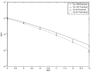
Figure 3: BER of the matched filter detector as a function of SNR, for an RCDMA system and a low pulse rate system

Figure 3 depicts the BER of the matched filter detector as a function of the SNR. We consider a three-user system, one user of which has SNR 3dB higher than the SNR of the other two. The curves shown correspond to an RCDMA system, that is $N_{f}=128$, and a system with pulse rate equal thirty two, that is $N_{f}=32$. The theoretical expressions for the BER are depicted as well.

As can be seen from the figure, the BER of the lower pulse rate system is lower than the BER of the RCDMA system, and a gain of more than 0.5dB can be achived by using the low pulse rate system. It is evident that the performance gap between the low pulse rate and high pulse rate system increases as the SNR increases. Recall that the self interference noise level increases as the pulse rate increases (see, (15). Therefore as long as the additive noise level and the MAI level are high compared with the self interference level, then the difference in BER of high and low pulse rate systems is negligible. However, when the SNR increases and the self interference noise becomes dominant, then the differences between low and high pulse rate systems become evident.

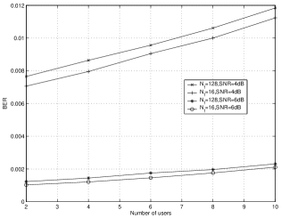
Figure 4: BER of the optimal MUD as a function of the number of users

In Figure 4 the optimal detector’s BER is depicted as a function of the number of users. We consider an RCDMA system and a low pulse rate system transmitting 16 pulses per symbol, with equal power users. We examined two SNRs 4dB and 6dB.

As can be seen from Fig 4 the BER increases as the number of users increases, and the low pulse rate system outperforms the RCDMA system for any number of users. In addition, it can be seen from the figure that for fixed SNR and BER the low pulse rate system can support two additional users compared with the RCDMA system.

In the last figure we examine the optimal detector’s BER as a function of the SNR and the pulse rate. We consider six equal power users, and an RCDMA system and two low pulse rate systems transmitting 32 and 8 pulses per symbol.

We can see from the figure that the RCDMA system requires an additional 0.3dB to achieve the same BER as the low pulse rate system. The performance improvement due to the use of low pulse rate system is not large. However, this performance improvement demonstrates the validity of our theoretical results as well asthe advantages of using low pulse rate systems.

IV Summary and Concluding Remarks

In this paper, the trade off between two types of processing gain, namly spreading and time division, has been analyzed under the assumption that the total processing gain is fixed and large. These two types of processing gain are interchangeable, and the analysis reveals that in some cases one should favor the second type of processing gain over the first.

Specifically, it has been argued that when coded systems transmitting over non-ISI channels are used, the two types of processing gains are reciprocal. That is, the BER of many MUDs is independent of the ratio between the two types of processing gain as long as the total processing gain is fixed. Nevertheless, the system complexity varies as the ratio between the two types of processing gain is changed. In systems that devote some of their processing gain to reducing the transmission time, the sampling rate can be decreased at the expense of large dynamic range requirements, when compared with high pulse rate systems.

In the context of UWB systems this result is very important. Under today’s regulations, the bandwidth of UWB systems could be up to $7\;GHz$. It is obvious that RCDMA systems that use the whole bandwidth will have to sample the received signal at rate of at least $7\;GHz$. On the other hand, some of the processing gain can be devoted to reducing the transmission time, and thus lower sampling rate could be used. Moreover, multiuser detection algorithms specifically designed for low pulse rate systems have very low complexity compared with their high pulse rate counterparts [5].

In frequency selective channels it has been shown that there is a tradeoff between the two types of processing gain, and this tradeoff is in favor of reducing the pulse rate, that is reducing the total transmission time. Although the decrease in the BER due to the use of low pulse rate systems can be low, the system complexity will be much lower than that of high pulse rate systems. It can be seen from the expression (15) for the approximate BER of the MF detector that the effect of the pulse rate on the total noise level is only via the signal transmitted from the user of interest. If the number of users is large or all the users transmit with equal power, the part of the noise level depending on the pulse rate is negligible compared to the part that is independent of the pulse level. In the equal-power-users case it is easy to verify that the part depending on the pulse rate is always smaller than the part independent of the pulse rate. Therefore, in these cases the advantage of the low pulse rate systems is negligible compared with high pulse rate systems.

Appendix A Proof of Lemma 1

Recall that
${\bm{\rho}}=[\rho_{1,1},\cdots,\rho_{K-1,K}]^{T}=\sum_{j=1}^{N}[s_{j}^{1}s_{j}^{2},\cdots,s_{j}^{K-1}s_{j}^{K}]^{T}=$
$\sum_{j=0}^{N_{f}-1}\sum_{l=1}^{N_{c}}[s_{jN_{c}+l}^{1}s_{jN_{c}+l}^{2},\cdots,s_{jN_{c}+l}^{K-1}s_{jN_{c}+l}^{K}]^{T}$. In order to prove the lemma we first show that for $m\neq n$ the random vectors $\sum_{l=1}^{N_{c}}[s_{mN_{c}+l}^{1}s_{mN_{c}+l}^{2},\cdots,s_{mN_{c}+l}^{K-1}s_{mN_{c}+l}^{K}]^{T}$ and $\sum_{l=1}^{N_{c}}[s_{nN_{c}+l}^{1}s_{nN_{c}+l}^{2},\cdots,s_{nN_{c}+l}^{K-1}s_{nN_{c}+l}^{K}]^{T}$ are independent and identically distributed with zero mean and covariance matrix equal $\frac{1}{N_{c}}{\bf I}$. It is easy to see from the definition of $s_{j}^{k}$ that, for every $k$, $s_{j}^{k}$ is independent of $s_{l}^{k}$ for $l\neq\lfloor j/N_{c}\rfloor N_{c}+1,\ldots,\lceil j/N_{c}\rceil N_{c}$. Thus, for $m\neq n$ the random variables $\{s_{mN_{c}+l}^{k}\}_{l=0,k=1}^{N_{c}-1,K}$ are jointly independent of $\{s_{nN_{c}+l}^{k}\}_{l=0,k=1}^{N_{c}-1,K}$, and so the random vectors $\sum_{l=1}^{N_{c}}[s_{mN_{c}+l}^{1}s_{mN_{c}+l}^{2},\cdots,s_{mN_{c}+l}^{K-1}s_{mN_{c}+l}^{K}]^{T}$ and $\sum_{l=1}^{N_{c}}[s_{nN_{c}+l}^{1}s_{nN_{c}+l}^{2},\cdots,s_{nN_{c}+l}^{K-1}s_{nN_{c}+l}^{K}]^{T}$ are independent as well. We now turn to examine the random variable $\sum_{l=1}^{N_{c}}s_{jN_{c}+l}^{n}s_{jN_{c}+l}^{m}$, where $0<n<m\leq K$ . This sum will be equal to zero if the $j$th pulse of the $m$th and $n$th users will be transmitted at different time slots. The probability of this event is $1-1/N_{c}$. If the $j$th pulse of the $m$th and $n$th users are transmitted at the same time slots, then the probability that both of them will transmit a pulse with equal phase is one-half. Combining these observations, it is easy to see that $\sum_{l=1}^{N_{c}}s_{jN_{c}+l}^{n}s_{jN_{c}+l}^{m}$ is a ternary random variable equaling zero with probability $1/N_{c}$, and one or minus one each with probability $1-1/(2N_{c})$. By using the same technique one can verify that the expectation of $\sum_{l=1}^{N_{c}}s_{jN_{c}+l}^{n}s_{jN_{c}+l}^{m}\sum_{l=1}^{N_{c}}s_{jN_{c}+l}^{k}s_{jN_{c}+l}^{l}$ equals zero.

Now, ${\bm{\rho}}=\sum_{j=1}^{N_{f}}{\bf V}_{j}^{T}$,
where ${\bf V}_{j}=\sum_{l=1}^{N_{c}}[s_{jN_{c}+l}^{1}s_{jN_{c}+l}^{2},\cdots,s_{jN_{c}+l}^{K-1}s_{jN_{c}+l}^{K}]^{T}$ is a zero mean random vector with covariance matrix $\frac{1}{N_{c}}{\bf I}$. Invoking the CLT on this sum proves the lemma; i.e.,

$$\sqrt{\frac{N_{c}}{N_{f}}}\rho\rightarrow N\left(0,{\bf I}\right)$$ (16)

Appendix B Analysis of the Matched Filter receiver in uncoded system

Define two functions $f_{1}(N_{c}),f_{2}(N_{c})$ as follow,

$$f_{1}(N_{c})=\frac{\sqrt{E_{1}}+\frac{\sqrt{E_{2}}}{N_{c}}}{\sqrt{\sigma^{2}+\frac{E_{2}}{N}\left(1-\frac{1}{N_{c}}\right)}}\quad;\quad f_{2}(N_{c})=\frac{\sqrt{E_{1}}-\frac{\sqrt{E_{2}}}{N_{c}}}{\sqrt{\sigma^{2}+\frac{E_{2}}{N}\left(1-\frac{1}{N_{c}}\right)}}.$$ (17)

The bit error rate (10) can be easily expressed with the aid $f_{1}(N_{c}),f_{2}(N_{c})$, and it is given by $P_{e}=1/2Q\left(f_{1}(N_{c})\right)+1/2Q\left(f_{2}(N_{c})\right)$. In what follows we find sufficient conditions such that the BER is a monotonically decreasing function of $N_{c}$, which is equivalent to proving that the BER is a monotonically increasing function of the pulse rate. In order to prove that the BER is a monotonically decreasing function of $N_{c}$ we first take the derivative of the BER with respect to $N_{c}$, which after some manipulation can be seen to be given by

$$\frac{\partial P_{e}}{\partial N_{c}}=\frac{\partial Q(f_{1}(N_{c}))+Q(f_{2}(N_{c}))}{\partial N_{c}}$$

$$=e^{-f_{1}^{2}(N_{c})}\left(\sigma^{2}+E_{2}N^{-1}-1/2E_{2}N^{-1}N_{c}^{-1}+1/2\sqrt{E_{1}E_{2}}N^{-1}\right)$$

$$-e^{-f_{2}^{2}(N_{c})}\left(\sigma^{2}+E_{2}N^{-1}-3/2E_{2}N^{-1}N_{c}^{-1}+1/2\sqrt{E_{1}E_{2}}N^{-1}\right).$$

In order for the BER to be a monotonically decreasing function of $N_{c}$, the derivative of the BER should be negative for every $N_{c}$. This is equivalent to the following condition,

$$f_{2}^{2}(N_{c})-f_{1}^{2}(N_{c})$$

$$<\ln\left(\frac{\sigma^{2}+E_{2}N^{-1}-3/2E_{2}N^{-1}N_{c}^{-1}1/2\sqrt{E_{1}E_{2}}N^{-1}}{\sigma^{2}+E_{2}N^{-1}-1/2E_{2}N^{-1}N_{c}^{-1}+1/2\sqrt{E_{1}E_{2}}N^{-1}}\right)$$

$$\quad,\quad\forall N_{c}.$$ (18)

Assume that $\frac{E_{1}}{N},\frac{E_{2}}{N}<\sigma^{2}$. Substituting (17) into (18), and by using our assumption, the following sufficient condition is deduced,

$$\frac{4\sqrt{E_{1}E_{2}}}{N_{c}\sigma^{2}+\frac{N_{c}E_{2}}{N}\left(1-\frac{1}{N_{c}}\right)}$$

$$>\ln\left(\frac{\sigma^{2}+E_{2}N^{-1}-1/2E_{2}N^{-1}N_{c}^{-1}}{\sigma^{2}+E_{2}N^{-1}-3/2E_{2}N^{-1}N_{c}^{-1}}\right)\quad,\forall N_{c}.$$ (19)

Upper bounding the right-hand side using the bound $\ln(1+x)<x$ results in the following sufficient condition,

$$\frac{4\sqrt{E_{1}}}{\sigma^{2}+\frac{E_{2}}{N}\left(1-\frac{1}{N_{c}}\right)}>\frac{\sqrt{E_{2}}N^{-1}}{\sigma^{2}+E_{2}N^{-1}-3/2E_{2}N^{-1}N_{c}^{-1}},\forall N_{c}.$$ (20)

Bounding the denominator of the left-hand side from above by $2\sigma^{2}$, and the denominator of the right hand side from below by $\sigma^{2}/2$, results in the following sufficient condition: $\sqrt{E_{1}}>\frac{\sqrt{E_{2}}}{N}$.

Appendix C Properties of the Correlation Coefficient in an Uncoded Systems

In this appendix the correlation between the spreading sequences of two uncoded users is examined. In particular, it is proven that, asymptotically in $N$, $\rho|N_{f}\preceq_{FSD}\rho|N_{f}^{\prime}$ for $1\leq N_{f}<N_{f}^{\prime}\leq N$, or equivalently that $\rho|N_{c}\succeq_{FSD}\rho|N_{c}^{\prime}$ for $1\leq N_{c}<N_{c}^{\prime}\leq N$, where $\preceq_{FSD}$ denotes first stochastic domination.

In order to prove that $\rho|N_{c}^{\prime}\preceq_{FSD}\rho|N_{c}$ we have to prove that for a fixed $x$, the probability of the event $\{(\rho|N_{c})\leq x\}$ is a monotonically increasing function of $N_{c}$. Recall that the correlation between the spreading sequences given $N_{c}$, $\rho|N_{c}$, is asymptotically normally distributed with mean $\frac{N_{f}}{N_{c}}$, and variance $\frac{N_{f}}{N_{c}}\left(1-\frac{1}{N_{c}}\right)$. Thus, the probability of the event $\{(\rho|N_{c})<x\}$ is, asymptotically, ${\textnormal{P}}\left((\rho|N_{f})<x\right)=1-Q\left(\frac{x-N_{f}/N_{c}}{\sqrt{N_{f}/N_{c}\left(1-1/N_{c}\right)}}\right)$. After some manipulation and using the relation $N_{f}N_{c}=N$, the asymptotic probability of error is thus given by

$${\textnormal{P}}\left((\rho|N_{c})<x\right)=1-Q\left(\frac{xN_{c}^{2}-N}{\sqrt{NN_{c}\left(N_{c}-1\right)}}\right).$$ (21)

Assume that $N_{c}>1$. In order to prove that (21) is a monotonically increasing function of $N_{c}$, it suffices to prove that the argument of the $Q$ function in (21) is a monotonically increasing function of $N_{c}$. Differentiating the argument of the $Q$ function in (21) with respect to $N_{c}$, and omitting some positive scaling factors, results in the following,

$$\frac{\partial}{\partial N_{c}}\frac{xN_{c}^{2}-N}{\sqrt{NN_{c}\left(N_{c}-1\right)}}$$

$$=4xNN_{c}^{2}(N_{c}-1)-\left(xN_{c}^{2}-N\right)\left(N(N_{c}-1)+NN_{c}\right)$$

$$=xN_{c}^{2}\left(2N_{c}-3\right)+N(2N_{c}-1).$$ (22)

It is easy to see that for $x\geq 0$, (22) is positive, and hence $\frac{xN_{c}^{2}-N}{\sqrt{NN_{c}\left(N_{c}-1\right)}}$ is a monotonically increasing function of $N_{c}$. Thus ${\textnormal{P}}\left((\rho|N_{c})<x\right)$ is a monotonically increasing function of $N_{c}$ as well. Note that since the system is an uncoded system, ${\textnormal{P}}\left((\rho|N_{c}<0)\right)=0$, so the case $x<0$, has no interest.

Assume that $N_{c}=1$. It is easy to verify that ${\textnormal{P}}\left((\rho|N_{c}=1)<x\right)=0$ for $x<N_{f}$ and ${\textnormal{P}}\left((\rho|N_{c}=1)<N_{f}\right)=1$. Combining this result with the monotonicity of ${\textnormal{P}}\left((\rho|N_{c})<\alpha\right)$ for $N_{c}>1$, concludes the proof.

Appendix D Properties of the interference

It is easy to verify from the definition of $d_{i}^{j}$ that the random variables $d_{j}^{1}d_{j-1}^{1},d_{j}^{1}d_{j}^{2},\mbox{ and }d_{j}^{1}d_{j-1}^{2}$ are binary random variables taking each of the values $\pm 1$ with probability 1/2. Let us derive the distribution of the random variable $h_{l}d_{i}^{1}d_{i-1}^{1}I_{1}$. The $(j-1)$th pulse transmitted by the first user will arrive via the second path at times when the $j$th pulse transmitted by the first user might be received if and only if $\prod_{m=1}^{N_{c}-l}s_{(j-1)N_{c}+m}^{1}=0$, and the probability of this event is $\frac{l}{N_{c}}$. Given that $\prod_{m=1}^{N_{c}-l}s_{(j-1)N_{c}+m}^{1}=0$ the probability that a collision will occur is $\frac{1}{N_{c}}$ (the probability of that arrival time of the $j$th pulse via the main path is equal to the arrival time of the $(j-1)$th pulse via the second path). Thus the probability of the event $\{I_{j}^{1}=1\}$ is $\frac{l}{N_{c}^{2}}$. Combining the distribution of $d_{j}^{1}d_{j-1}^{1}$ and the distribution of $I_{j}^{1}$ results in the following distribution for $h_{l}d_{j}^{1}d_{j-1}^{1}I_{j}^{1}$: $h_{l}d_{j}^{1}d_{j-1}^{1}I_{j}^{1}$ can take on the values $h_{l},0,-h_{l}$ with probabilities $1/(2N_{c}^{2}),1-1/(N_{c}^{2}),1/(2N_{c}^{2})$ respectively. It is easy to show in a similar way that the marginal distribution of $h_{l}d_{j}^{1}d_{j-1}^{2}I_{j}^{3}$ is equal to the marginal distribution of $h_{l}d_{j}^{1}d_{j-1}^{1}I_{j}^{1}$.

Similar arguments can lead to the following marginal distribution of $d_{j}^{1}d_{j}^{2}I_{j}^{2}$: $d_{j}^{1}d_{j}^{2}I_{j}^{2}$ takes on the values $1,h_{l},0,-h_{l},-1$ with probabilities $1/(2N_{c}),1/(2N_{c})-l/(2N_{c}^{2}),1-2/N_{c}+j/N_{c}^{2},1/(2N_{c})-l/(2N_{c}^{2}),1/(2N_{c})$, respectively. It is easy to verify that $\{h_{l}d_{j}^{1}d_{j-1}^{1}I_{j}^{1}\}$, $\{d_{j}^{1}d_{j}^{2}I_{j}^{3}\}$, $\{h_{l}d_{j}^{1}d_{j-1}^{2}I_{j}^{3}\}$ are zero mean white, mutually uncorrelated random sequences. For example take $h_{l}d_{j}^{1}d_{j-1}^{1}I_{j}^{1}$, and let $j$ and $k$ be two distinct time indices. The mean of $h_{l}d_{j}^{1}d_{j-1}^{1}I_{j}^{1}\cdot h_{l}d_{k}^{1}d_{k-1}^{1}I_{k}^{1}$ is

$$E\left\{h_{l}^{2}d_{j}^{1}d_{j-1}^{1}I_{j}^{1}d_{k}^{1}d_{k-1}^{1}I_{k}^{1}\right\}=E\left\{d_{j}^{1}\right\}E\left\{h_{l}^{2}d_{j-1}^{1}I_{j}^{1}d_{k}^{1}d_{k-1}^{1}I_{k}^{1}\right\}=0$$ (23)

where for the last equality we used the fact the $d_{j}^{1}$ is independent of all the other random variables, and we assumed that $j\neq k-1$ (if $j=k-1$, take $d_{k-1}^{1}$ instead).

The total interference is given by
$\sum_{j=1}^{N_{f}}\left[\sqrt{\frac{E_{1}}{N_{f}}}h_{l}d_{j}^{1}d_{j-1}^{1}I_{j}^{1}+\sqrt{\frac{E_{2}}{N_{f}}}d_{j}^{1}d_{j}^{2}I_{j}^{2}+\sqrt{\frac{E_{2}}{N_{f}}}h_{l}d_{j}^{1}d_{j-1}^{2}I_{j}^{3}\right]$. Since the three random processes $\{h_{l}d_{j}^{1}d_{j-1}^{1}I_{j}^{1}\}$, $\{d_{j}^{1}d_{j}^{2}I_{j}^{3}\}$, $\{h_{l}d_{j}^{1}d_{j-1}^{2}I_{j}^{3}\}$ are zero mean and mutually uncorrelated, the mean and the variance of $\sqrt{\frac{E_{1}}{N_{f}}}h_{l}d_{j}^{1}d_{j-1}^{1}I_{j}^{1}+\sqrt{\frac{E_{2}}{N_{f}}}d_{j}^{1}d_{j}^{2}I_{j}^{2}+\sqrt{\frac{E_{2}}{N_{f}}}h_{l}d_{j}^{1}d_{j-1}^{2}I_{j}^{3}$ are zero and $\frac{E_{1}}{N_{f}}\frac{h_{l}^{2}l}{N_{c}^{2}}+\frac{E_{2}}{N_{f}}\frac{1+h_{l}^{2}}{N_{c}}$, respectively. Although $\left\{\sqrt{\frac{E_{1}}{N_{f}}}h_{l}d_{j}^{1}d_{j-1}^{1}I_{j}^{1}+\sqrt{\frac{E_{2}}{N_{f}}}d_{j}^{1}d_{j}^{2}I_{j}^{2}+\sqrt{\frac{E_{2}}{N_{f}}}h_{l}d_{j}^{1}d_{j-1}^{2}I_{j}^{3}\right\}$ is a white random sequence, it is not an independent one. Nevertheless, it is a $1$-dependent random sequence, and hence it is a $\phi$-mixing random sequence for which the conditions in [1] hold. Thus, a central limit theorem can be invoked, implying the asymptotic normality of the total interference,

$$\sum_{j=1}^{N_{f}}\sqrt{\frac{E_{1}}{N_{f}}}h_{l}d_{j}^{1}d_{j-1}^{1}I_{i}^{1}+\sqrt{\frac{E_{2}}{N_{f}}}d_{j}^{1}d_{j}^{2}I_{j}^{2}$$

$$+\sqrt{\frac{E_{2}}{N_{f}}}h_{l}d_{j}^{1}d_{j-1}^{2}I_{j}^{3}\sim{\mathcal{N}}\left(0,\frac{2E_{1}h_{l}^{2}l}{N_{c}^{2}}+E_{2}\frac{1+h_{l}^{2}}{N_{c}}\right).$$ (24)

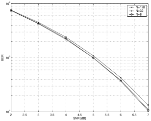
Figure 5: BER of the optimal MUD as a function of the SNR

References

- [1] P. Bilingsly. Probability and Measure. John Wiley & Sons, New York, 2nd edition, 1986.
- [2] D. Cassioli, M. Z. Win, and A. F. Molisch. The Ultra-Wide Bandwidth Indoor Channel: From Statistical Model to Simulations. IEEE J. Select. Areas Commun., 20(9):1247–1257, Dec. 2002.
- [3] R. J. Cramer, R. A. Scholtz, and M. Z. Win. An Evaluation of The Ultra-Wideband Propagation Channel. IEEE Trans. Antennas Propagat., 50(5):561–570, May 2002.
- [4] J. Evans and D. N. C. Tse. Large System Performance of Linear Multiuser Receivers in Multipath Fading Channels. IEEE Trans. Inform. Theory, IT-46(6):2059–2078, September 2000.
- [5] E. Fishler and H. V. Poor. Low-Complexity Multi-User Detection in Time Hopping Impulse Radio System. IEEE Trans. on Signal Processing (to appear), 2004.
- [6] E. Fishler and H. V. Poor. On The Tradeoff Between Two Types of Processing Gain. In Proceedings of the 40th Annual Allerton Conference on Communication, Control, and Computing, Allerton Park, IL, October, 2002.
- [7] C. J. Le-Martret and G. B. Giannakis. All-Digital PAM Impulse Radio for Multiple-Access Through Frequency-Selective Multipath. In Proceedings of the 2000 IEEE Global Telecommunications Conference (GLOBECOM2000), volume 1, pages 77–81, San Francisco, CA, Nov. 2000.
- [8] T. S. Rappaport. Wireless Communications: Principles and Practice. Prentice Hall, 2nd edition, Upper Saddle River, NJ, 2001.
- [9] B. Sadler and A. Swami. On the Performance of UWB and DS-Spread Spectrum Communication Systems. In Proceedings of the IEEE Conference on Ultra Wideband Systems and Technologies (UWBST02), pages 289–292, Baltimore, MD, May 2002.
- [10] R. A. Scholtz. Multiple Access with Time-Hopping Impulse Modulation. In Proceedings of the IEEE Military Communications Conference, (MILCOM 93), volume 2, pages 447–450, Boston, MA, Oct. 1993.
- [11] D. Tse and S. Hanly. Linear Multiuser Receivers: Effective Interference, Effective Bandwidth and User Capacity. IEEE Trans. on Inform. Theory, IT-45(2):641–657, March 1999.
- [12] S. Verd. Multiuser Detection. Cambridge University Press, Cambridge, UK, 1998.
- [13] S. Verd and S. Shamai (Shitz). Spectral Efficiency of CDMA with Random Spreading. IEEE Trans. on Inform. Theory, IT-45(2):622–640, March 1999.
- [14] G. A. Whitmore and M. C. Findlay. Stochastic Dominance. Lexington Books, Lexington, MA, 1982.
- [15] M. Z. Win and R. A. Scholtz. Impulse Radio: How It Works. IEEE Communications Letters, 2(2):36–38, Feb. 1998.
- [16] M. Z. Win and R. A. Scholtz. On Energy Capture of Ultra-Wide Bandwidth Signals in Dense Multipath Environments. IEEE Commun. Lett., 2(9):245–247, Sept. 1998.
- [17] M. Z. Win and R. A. Scholtz. Ultra-Wide Bandwidth Time-Hopping Spread-Spectrum Impulse Radio for Wireless Multiple Access Communications. IEEE Trans. Commun., COM-48(4):679–689, April 2000.
- [18] M. Z. Win and R. A. Scholtz. Characterization of Ultra-Wide Bandwidth Wireless Indoor Communications Channel: A Communication Theortic View. IEEE J. Select. Areas Commun, 20(9):1613–1627, Dec. 2002.
- [19] M. Z. Win and R.A. Scholtz. On The Robustness of Ultra-Wide Bandwidth Signals in Dense Multipath Environments. IEEE Commun. Lett., 2(2):51–53, Feb. 1998.