Large-scale lattice Boltzmann simulations of complex fluids: advances through the advent of computational grids

Abstract

Lattice-Boltzmann, complex fluids, grid computing, computational steering

During the last two years the RealityGrid project has allowed us to be one of the few scientific groups involved in the development of computational grids. Since smoothly working production grids are not yet available, we have been able to substantially influence the direction of software development and grid deployment within the project. In this paper we review our results from large scale three-dimensional lattice Boltzmann simulations performed over the last two years. We describe how the proactive use of computational steering and advanced job migration and visualization techniques enabled us to do our scientific work more efficiently. The projects reported on in this paper are studies of complex fluid flows under shear or in porous media, as well as large-scale parameter searches, and studies of the self-organisation of liquid cubic mesophases.

1 Introduction

In recent years there has emerged a class of fluid dynamical problems, called “complex fluids”, which involve both hydrodynamic flow effects and complex interactions between fluid particles. Computationally, such problems are too large and expensive to tackle with atomistic methods such as molecular dynamics, yet they require too much molecular detail for continuum Navier-Stokes approaches.

Algorithms which work at an intermediate or “mesoscale” level of description in order to solve these problems have been developed in response, including Dissipative Particle Dynamics[Espa$\tilde{\mbox{n}}$ol and Warren, 1995, Jury et al., 1999, Flekkøy et al., 2000], Lattice Gas Cellular Automata[Rivet and Boon, 2001], the Stochastic Rotation Dynamics of Malevanets and Kapral[Malevanets and Kapral, 1998, Hashimoto et al., 2000, Sakai et al., 2000], and the Lattice Boltzmann Equation[Succi, 2001, Benzi et al., 1992, Love et al., 2003]. In particular, the Lattice Boltzmann method has been found highly useful for simulation of complex fluid flows in a wide variety of systems. This algorithm, described in more detail below, is extremely well suited to implementation on parallel computers, which permits very large systems to be simulated, reaching hitherto inaccessible physical regimes. We describe some of these calculations, and also attempts to take parallel computing to a new scale, by coupling several supercomputers together into a computational grid, which in turn permits easy use of techniques such as computational steering, code migration, and real-time visualization.

The term “simple fluid” usually refers to a fluid which can be described to a good degree of approximation by macroscopic quantities only, such as the density field $\rho(\bf{x})$, velocity field $\bf{v}(\bf{x})$, and perhaps temperature $T(\bf{x})$. Such fluids are governed by the well-known Navier-Stokes equations[Faber, 1995], which, being nonlinear, are difficult to solve in the most general case, with the result that numerical solution of the equations has become a common tool for understanding the behaviour of “simple” fluids, such as water or air. Conversely, a “complex fluid” is one whose macroscopic flow is affected by its microscopic properties. A good example of such a fluid is blood: as it flows through vessels (of order millimetres wide and centimetres long), it is subjected to shear forces, which cause red blood cells (of order micrometres wide) to align with the flow so that they can slide over one another more easily, causing the fluid to become less viscous; this change in viscosity in turn affects the flow profile. Hence, the macroscopic blood flow is affected by the microscopic alignment of its constituent cells. Other examples of complex fluids include biological fluids such as milk, cell organelles and cytoplasm, as well as polymers and liquid crystals. In all of these cases, the density and velocity fields are insufficient to describe the fluid behaviour, and in order to understand this behaviour, it is necessary to treat effects which occur over a very wide range of length and time scales. This length and time scale gap makes complex fluids even more difficult to model than “simple” fluids. While numerical solutions of the macroscopic equations are possible for many simple fluids, such a level of description may not exist for complex fluids, yet simulation of every single molecule involved is computationally infeasible.

In a mixture containing many different fluid components, an amphiphile is a kind of molecule which is composed of two parts, each part being attracted towards a different fluid component. For example, soap molecules are amphiphiles, containing a head group which is attracted towards water, and a tail which is attracted towards oil and grease; analogous molecules can also be formed from polymers. If many amphiphile molecules are collected together in solution, they can exhibit highly varied and complicated behaviour, often assembling to form amphiphile mesophases, which are complex fluids of significant theoretical and industrial importance. Some of these phases have long-range order, yet remain able to flow, and are called liquid crystal mesophases. Of particular interest to us are those with cubic symmetry, whose properties have been studied experimentally [Seddon and Templer, 1995, Seddon and Templer, 1993, Czeslik and Winter, 2002] in lipid-water mixtures[Seddon and Templer, 1995], diblock copolymers[Shefelbine et al., 1999], and in many biological systems[Landh, 1995].

Over the last decade, significant effort has been invested in understanding complex fluids through computational mesoscale modelling techniques. These techniques do not attempt to keep track of the state of every single constituent element of a system, nor do they use an entirely macroscopic description; instead, an intermediate, mesoscale model of the fluid is developed, coarse-graining microscopic interactions enough that they are rendered amenable to simulation and analysis, but not so much that the important details are lost. Such approaches include Lattice Gas Automata[Rivet and Boon, 2001, Frisch et al., 1986, Rothman and Keller, 1988, Love, 2002], the Lattice Boltzmann equation[Succi, 2001, Benzi et al., 1992, McNamara and Zanetti, 1988, Higuera and Jiménez, 1989, Higuera et al., 1989, Shan and Chen, 1993, Lamura et al., 1999, Chen et al., 2000, Chin and Coveney, 2002], Dissipative Particle Dynamics[Hoogerbrugge and Koelman, 1992, Espa$\tilde{\mbox{n}}$ol and Warren, 1995, Jury et al., 1999], or the Malevanets-Kapral Real-coded Lattice Gas[Malevanets and Kapral, 1998, Malevanets and Yeomans, 2000, Hashimoto et al., 2000, Sakai et al., 2000]. Recently-developed techniques[Garcia et al., 1999, Delgado-Buscalioni and Coveney, 2003] which use hybrid algorithms have shown much promise.

All simulations described in this paper use the lattice Boltzmann algorithm, which is a powerful method for simulating fluid dynamics. This is due to the ease with which boundary conditions can be imposed, and with which the model may be extended to describe mixtures of interacting complex fluids. Rather than tracking the state of individual atoms and molecules, the method describes the dynamics of the single-particle distribution function of mesoscopic fluid packets.

In a continuum description, the single-particle distribution function $f_{1}({{\bf r}},{{\bf v}},t)$ represents the density of fluid particles with position ${{\bf r}}$ and velocity ${{\bf v}}$ at time $t$, such that the density and velocity of the macroscopically observable fluid are given by $\rho({{\bf r}},t)=\int f_{1}({{\bf r}},{{\bf v}},t){\mathrm{d}}{{\bf v}}$ and ${{\bf u}}({{\bf r}},t)=\int f_{1}({{\bf r}},{{\bf v}},t){{\bf v}}{\mathrm{d}}{{\bf v}}$ respectively. In the non-interacting, long mean free path limit, with no externally applied forces, the evolution of this function is described by Boltzmann’s equation,

$$\left(\partial_{t}+{{\bf v}}\cdot{{\bf\nabla}}\right)f_{1}=\Omega[f_{1}].$$ (1)

While the left hand side describes changes in the distribution function due to free particle motion, the right hand side models pairwise collisions. This collision operator $\Omega$ is an integral expression that is often simplified [Bhatnagar et al., 1954] to the linear Bhatnagar-Gross-Krook (BGK) form

$$\Omega[f]\simeq-\frac{1}{\tau}\left[f-f^{\mathrm{(eq)}}\right].$$ (2)

The BGK collision operator describes the relaxation, at a rate controlled by a characteristic time $\tau$, towards a Maxwell-Boltzmann equilibrium distribution $f^{\mathrm{(eq)}}$. While this is a drastic simplification, it can be shown that distributions governed by the Boltzmann-BGK equation conserve mass, momentum, and energy [Succi, 2001], and obey a non-equilibrium form of the Second Law of Thermodynamics [Liboff, 1990]. Moreover, it can be shown [Chapman and Cowling, 1952, Liboff, 1990] that the well-known Navier-Stokes equations for macroscopic fluid flow are obeyed on coarse length and time scales [Chapman and Cowling, 1952, Liboff, 1990]. In a lattice Boltzmann formulation, the single-particle distribution function is discretized in time and space. The positions ${{\bf r}}$ on which $f_{1}({{\bf r}},{{\bf v}},t)$ is defined are restricted to points ${{\bf r}}_{i}$ on a lattice, and the velocities ${{\bf v}}$ are restricted to a set ${{{\bf c}}_{i}}$ joining points on the lattice. The density of particles at lattice site ${{\bf r}}$ travelling with velocity ${{{\bf c}}_{i}}$, at timestep $t$ is given by $f_{i}({{\bf r}},t)=f({{\bf r}},{{{\bf c}}_{i}},t)$, while the fluid’s density and velocity are given by $\rho({{\bf r}})=\sum_{i}f_{i}({{\bf r}})$ and ${{\bf u}}({{\bf r}})=\sum_{i}f_{i}({{\bf r}}){{{\bf c}}_{i}}$. The discretized description can be evolved in two steps: the collision step, where particles at each lattice site are redistributed across the velocity vectors, and the advection, where values of the post-collisional distribution function are propagated to adjacent lattice sites. By combining these steps, one obtains the lattice-Boltzmann equation (LBE)

$$f_{i}({{\bf r}},t+1)-f_{i}({{\bf r}},t)=\Omega[f]\\ =-\frac{1}{\tau}\left[f_{i}({{\bf r}},t)-N_{i}\left(\rho,{{\bf u}}\right)\right],$$ (3)

where $N_{i}=N_{i}\left(\rho({{\bf r}}),{{\bf u}}({{\bf r}})\right)$ is a polynomial function of the local density and velocity, which may be found by discretizing the well-known Maxwell-Boltzmann equilibrium distribution. Our implementation uses the Shan-Chen approach [Shan and Chen, 1993], by incorporating an explicit forcing term in the collision operator in order to model multicomponent interacting fluids. Shan and Chen extended $f_{i}$ to the form $f_{i}^{\sigma}$, where each component is denoted by a different value of the superscript $\sigma$, so that density and momentum of a component $\sigma$ are given by $\rho^{\sigma}=\sum_{i}f_{i}^{\sigma}$ and $\rho^{\sigma}{{\bf u}}^{\sigma}=\sum_{i}f_{i}^{\sigma}{{{\bf c}}_{i}}$. The fluid viscosity $\nu^{\sigma}$ is proportional to $(\tau^{\sigma}-1/2)$ and the particle mass is $m^{\sigma}$. This results in a lattice BGK equation (3) of the form

$$f_{i}^{\sigma}({{\bf r}},t+1)-f_{i}^{\sigma}({{\bf r}},t)=-\frac{1}{\tau^{\sigma}}\left[f_{i}^{\sigma}-N_{i}(\rho^{\sigma},{{\bf v}}^{\sigma})\right]$$ (4)

The velocity ${{\bf v}}^{\sigma}$ is found by calculating a weighted average velocity ${{\bf u}}^{\prime}$ and then adding a term to account for external forces:

$${{\bf u}}^{\prime}=\left(\sum_{\sigma}\frac{\rho^{\sigma}}{\tau^{\sigma}}{{\bf u}}^{\sigma}\right)/\left(\sum_{\sigma}\frac{\rho^{\sigma}}{\tau^{\sigma}}\right),\qquad{{\bf v}}^{\sigma}={{\bf u}}^{\prime}+\frac{\tau^{\sigma}}{\rho^{\sigma}}{{\bf F}}^{\sigma}.$$ (5)

In order to produce nearest-neighbour interactions between components, the force term assumes the form

$${{\bf F}}^{\sigma}=-\psi^{\sigma}({{\bf x}})\sum_{\bar{\sigma}}g_{\sigma\bar{\sigma}}\sum_{i}\psi^{\bar{\sigma}}\left({{\bf x}}+{{{\bf c}}_{i}}\right){{{\bf c}}_{i}},$$ (6)

where $\psi^{\sigma}({{\bf x}})=\psi^{\sigma}(\rho^{\sigma}({{\bf x}}))$ is an effective charge for component $\sigma$; $g_{\sigma\bar{\sigma}}$ is a coupling constant controlling the strength of the interaction between two components $\sigma$ and $\bar{\sigma}$. If $g_{\sigma\bar{\sigma}}$ is set to zero for $\sigma=\bar{\sigma}$, and a positive value for $\sigma\neq\bar{\sigma}$ then, in the interface between bulk regions of each component, particles experience a force in the direction away from the interface, producing immiscibility. In two-component systems, it is usually the case that $g_{\sigma\bar{\sigma}}=g_{\bar{\sigma}\sigma}=g_{br}$. Amongst other things, this model has been used to simulate spinodal decomposition [Chin and Coveney, 2002, González-Segredo et al., 2003], polymer blends [Martys and Douglas, 2001], liquid-gas phase transitions [Shan and Chen, 1994], and flow in porous media [Martys and Chen, 1996]. Amphiphilic fluids may be treated by introducing a new species of particle with an orientational degree of freedom, which is modelled by a vector dipole moment ${{\bf d}}$ [Chen et al., 2000] with magnitude $d_{0}$. The dipole field ${{\bf d}}({{\bf x}},t)$ represents the average orientation of any amphiphile present at site ${{\bf x}}$. During advection, values of ${{\bf d}}({{\bf x}},t)$ are propagated according to (tildes denote post-collision values)

$$\rho^{\mathrm{s}}({{\bf x}},t+1){{\bf d}}({{\bf x}},t+1)=\sum_{i}\tilde{f_{i}^{\mathrm{s}}}({{\bf x}}-{{{\bf c}}_{i}},t)\tilde{{{\bf d}}}({{\bf x}}-{{{\bf c}}_{i}},t),$$ (7)

During collision, the dipole moments evolve in a BGK process controlled by a dipole relaxation time $\tau_{d}$:

$$\tilde{{{\bf d}}}({{\bf x}},t)={{\bf d}}({{\bf x}},t)-\frac{1}{\tau_{d}}\left[{{\bf d}}({{\bf x}},t)-{{\bf d}}^{\mathrm{(eq)}}({{\bf x}},t)\right].$$ (8)

The equilibrium dipole moment ${{\bf d}}^{\mathrm{(eq)}}\simeq{\beta d_{0}}{{\bf h}}/3$ is aligned with the colour field ${{\bf h}}$ which contains a component ${{\bf h}}^{c}$ due to coloured particles, and a part ${{\bf h}}^{s}$ due to dipoles. With $q^{\sigma}$ being a colour charge, such as $+1$ for red particles, $-1$ for blue particles, and $0$ for amphiphile particles, one gets

$${{\bf h}}^{c}=\sum_{\sigma}q^{\sigma}\sum_{i}\rho^{\sigma}({{\bf x}}+{{{\bf c}}_{i}}){{{\bf c}}_{i}},$$ (9)

$${{\bf h}}^{s}({{\bf x}},t)=\sum_{i}\left[\sum_{j\neq 0}f_{i}^{s}({{\bf x}}+{{{\bf c}}_{i}},t){{\bf\theta}}_{j}\cdot{{\bf d}}_{i}({{\bf x}}+{{\bf c}}_{j},t)+f_{i}^{s}({{\bf x}},t){{\bf d}}_{i}({{\bf x}},t)\right].$$ (10)

The second-rank tensor ${{\bf\theta}}_{j}$ is defined in terms of the unit tensor ${{\bf I}}$ and lattice vector ${{\bf c}}_{j}$ as ${{\bf\theta}}_{j}={{\bf I}}-D{{\bf c}}_{j}{{\bf c}}_{j}/{c^{2}}$. In the presence of an amphiphilic species, the force on a coloured particle includes an additional term ${{\bf F}}^{\sigma,s}$ to account for the colour field due to the amphiphiles. By treating an amphiphilic particle as a pair of oil and water particles with a very small separation ${{\bf d}}$, introducing a constant $g_{\sigma s}$ to control the strength of the interaction between amphiphiles and non-amphiphiles and Taylor-expanding in ${{\bf d}}$, it can be shown that this term is given by

$${{\bf F}}^{\sigma,s}({{\bf x}},t)=-2\psi^{\sigma}({{\bf x}},t)g_{\sigma s}\sum_{i\neq 0}\tilde{{{\bf d}}}({{\bf x}}+{{{\bf c}}_{i}},t)\cdot{{\bf\theta}}_{i}\psi^{s}({{\bf x}}+{{{\bf c}}_{i}},t).$$ (11)

While amphiphiles do not possess a net colour charge, they also experience a force due to the colour field, consisting of a part ${{\bf F}}^{s,c}$ due to ordinary species, and a part ${{\bf F}}^{s,s}$ due to other amphiphiles:

$${{\bf F}}^{s,c}=2\psi^{s}({{\bf x}},t)\tilde{{{\bf d}}}({{\bf x}},t)\cdot\sum_{\sigma}g_{\sigma s}\sum_{i\neq 0}{{\bf\theta}}_{i}\psi^{\sigma}({{\bf x}}+{{{\bf c}}_{i}},t),$$ (12)

$${{\bf F}}^{s,s} = -\frac{4D}{c^{2}}g_{ss}\psi^{s}({{\bf x}})\sum_{i}\left\{\tilde{{{\bf d}}}({{\bf x}}+{{{\bf c}}_{i}})\cdot{{\bf\theta}}_{i}\cdot\tilde{{{\bf d}}}({{\bf x}}){{{\bf c}}_{i}}\right.$$

$$+ \left.\left[\tilde{{{\bf d}}}({{\bf x}}+{{{\bf c}}_{i}})\tilde{{{\bf d}}}({{\bf x}})+\tilde{{{\bf d}}}({{\bf x}})\tilde{{{\bf d}}}({{\bf x}}+{{{\bf c}}_{i}})\right]\cdot{{{\bf c}}_{i}}\right\}\psi^{s}({{\bf x}}+{{{\bf c}}_{i}}).$$

While the form of the interactions seems straightforward at a mesoscopic level, it is essentially phenomenological, and it is not necessarily easy to relate the interaction scheme or its coupling constants to either microscopic molecular characteristics, or to macroscopic phase behaviour. The phase behaviour can be very difficult to predict beforehand from the simulation parameters, and brute-force parameter searches are often resorted to [Boghosian et al., 2000].

2 Technical projects

Our three-dimensional lattice Boltzmann code, LB3D, is written in Fortran 90 and designed to run on distributed-memory parallel computers, using MPI for communication. In each simulation, the fluid is discretized onto a cuboidal lattice, each lattice point containing information about the fluid in the corresponding region of space. Each lattice site requires about a kilobyte of memory per lattice site so that, for example, a simulation on a $128^{3}$ lattice would require around $2.2{\mathrm{GB}}$ memory. The high-performance computing machines on which most of the simulation work is performed are typically rather heavily used The situation frequently arises that while a simulation is running on one machine, CPU time becomes available on another machine which may be able to run the job faster or cheaper. The LB3D program has the ability to “checkpoint” its entire state to a file. This file can then be moved to another machine, and the simulation restarted there, even if the new machine has a different number of CPUs or even a completely different architecture. It has been verified that the simulation results are independent of the machine on which the calculation runs, so that a single simulation may be migrated between different machines as necessary without affecting its output. As a conservative rule of thumb, the code runs at over $10^{4}$ lattice site updates per second per CPU on a fairly recent machine, and has been observed to have roughly linear scaling up to order $10^{3}$ compute nodes. A $128^{3}$ simulation contains around $2.1\times 10^{6}$ lattice sites; running it for 1000 timesteps requires about an hour of real time, split across $64$ CPUs. The largest simulation we performed used a $1024^{3}$ lattice. The output from a simulation usually takes the form of a single floating-point number for each lattice site, representing, for example, the density of a particular fluid component at that site. Therefore, a density field snapshot from a $128^{3}$ system would produce output files of around $8{\mathrm{MB}}$. Writing data to disk is one of the bottlenecks in large scale simulations. If one simulates a 1024³ system, each data file is $4{\mathrm{GB}}$ in size. LB3D is able to benefit from the parallel filesystems available on many large machines today, by using the MPI-IO based parallel HDF5 data format [HDF5, 2003]. Our code is very robust regarding different platforms or cluster interconnects: even with moderate inter-node bandwidths it achieves almost linear scaling for large processor counts with the only limitation being the available memory per node. The platforms our code has been successfully used on include various supercomputers like the IBM pSeries, SGI Altix and Origin, Cray T3E, Compaq Alpha clusters, NEC SX6, as well as low cost 32- and 64-bit Linux clusters. However, due to compiler or machine peculiarities it is a time consuming task to achieve optimum performance on many different platforms. Porting a complex Fortran code like LB3D to new platforms is often very difficult and time-consuming without the assistance of well trained staff at the corresponding computer centres. Some of these problems are due to portability issues with the Fortran language. Also, tuning a code to take full advantage of the machine on which it runs requires considerable knowledge of the local system’s quirks. It is hoped that some of the portability issues could be solved in future by well-designed middleware. Such issues include the fact that location, size, and duration of temporary filespace change from machine to machine, as do the methods for invoking compilers and batch queues.

LB3D has successfully been used to study various problems like spinodal decomposition with and without shear [González-Segredo et al., 2003, Harting et al., 2004b], flow in porous media [Harting et al., 2004b], the self-assembly of cubic mesophases such as the ’P’-phase [Nekovee and Coveney, 2001a] in binary water-surfactant systems, or the cubic gyroid phase in ternary amphiphilic systems [González-Segredo and Coveney, 2004b, González-Segredo and Coveney, 2004a]. Before we were able to take advantage of computational steering techniques, our work usually involved large scale parameter searches organised as taskfarming jobs in order to find the areas of interest of the available parameter space. The technique of computational steering[Chin et al., 2003, Brooke et al., 2003, Love et al., 2003] has been used successfully in smaller-scale simulations to optimize resource usage. Typically, the procedure for running a simulation of the self-assembly of a mesophase would be to set up the initial conditions, and then submit a batch job to run for a certain, fixed number of timesteps. If the timescale for structural assembly is unknown then the initial number of timesteps for which the simulation runs is, at best, an educated guess. It is not uncommon to examine the results of such a simulation once they return from the batch queue, only to find that a simulation has not been run for sufficient time (in which case it must be tediously resubmitted), or that it ran for too long, and the majority of the computer time was wasted on simulation of an uninteresting equilibrium system showing no dynamical behaviour. Another unfortunate scenario often occurs when the phase diagram of a simulated system is not well known, in which case a simulation may evolve away from a situation of interest, wasting further CPU time. Computational steering, the ability to watch and control a calculation as it runs, can be used to avoid these difficulties: a simulation which has equilibrated may be spotted and terminated, preventing wastage of CPU time. More powerfully, a simulation may be steered through parameter space until it is unambiguously seen to be producing interesting results: this technique is very powerful when searching for emergent phenomena, such as the formation of surfactant micelles, which are not clearly related to the underlying simulation parameters. Steering is performed using the RealityGrid steering library which has been developed by collaborators at the University of Manchester. The library was built with the intention of making it possible to add steering capabilities to existing simulation codes with as few changes as possible, and in as general a manner as possible. Once the application has initialized the steering library and informed it which parameters are to be steered, then after every timestep of the simulation, it is possible to perform tasks such as checkpointing the simulation, saving output data, stopping the simulation, or restarting from an existing checkpoint. When a steered simulation is started, a Steering Grid Service (SGS) is also created, to represent the steerable simulation on the Grid. The SGS publishes its location to a Registry service, so that steering clients may find it. This design means that it is possible for clients to dynamically attach to and detach from running simulations.

Successful computational steering requires that the simulation operators have a good understanding of what the simulation is doing, in real time: this in turn requires good visualization capabilities. Each running simulation emits output files after certain periods of simulation time have elapsed. The period between output emission is initially determined by guessing a timescale over which the simulation will change in a substantial way; however, this period is a steerable parameter, so that the output rate can be adjusted for optimum visualization without producing an excessive amount of data. The LB3D code itself will only emit volumetric datasets as described above; these must then be rendered into a human-comprehensible form through techniques including volume-rendering, isosurfacing, ray-tracing, slice planes, and Fourier transforms. The process of producing such comprehensible data from the raw datasets is itself computationally intensive, particularly if it is to be performed in real time, as required for computational steering. For this reason, we use separate visualization clusters to render the data. Output volumes are sent from the simulation machine to the remote visualization machine, so that the simulation can proceed independently of the visualization; these are then rendered using the open source VTK[Schroeder et al., 2003] visualization library into bitmap images, which can in turn be multicast over the AccessGrid, so that the state of the simulation can be viewed by scientists around the globe. In particular, this was demonstrated by performing and interacting with a simulation in front of a live worldwide audience, as part of the SCGlobal track of the SuperComputing 2004 conference. The RealityGrid steering architecture was designed in a sufficiently general manner that visualization services can also be represented by Steering Grid Services: in order to establish a connection between the visualization process and the corresponding simulation, the simulation SGS can be found through the Registry, and then interrogated for the information required to open the link.

In order to be able to deploy the above described components as part of a usable simulation Grid, a substantial amount of coordination is necessary, so that the end user is able to launch an entire simulation pipeline, containing migratable simulation, visualization, and steering components, from a unified interface. This requires a system for keeping track of which services are available, which components are running, taking care of the checkpoints and data which are generated, and to harmonize communication between the different components. This was achieved through the development of a Registry service, implemented using the OGSI: ​​​​:Lite [McKeown, 2003] toolkit. The RealityGrid steering library[Chin et al., 2003] communicates with the rest of the Grid by exposing itself as a “Grid Service”. Through the Registry service, steering clients are able to find, dynamically attach to, communicate with, and detach from steering services to control a simulation or visualization process.

Large lattices require a highly scalable code, access to high performance computing, terascale storage facilities and high performance visualisation. LB3D provides the first of these, while the others are being delivered by the major computing centres. We expect to be able to run our simulations in an even more efficient way due to the significant worldwide effort being invested in the development of reliable computational grids. These are a collection of geographically distributed and dynamically varying resources, each providing services such as compute cycles, visualization, storage, or even experimental facilities. The major difference between computational grids and traditional distributed computing is the transparent sharing and collective use of resources, which would otherwise be individual and isolated facilities. Perhaps at some point computational grids will offer information technology what electricity grids offer for other aspects of our daily life: a transparent and reliable resource that is easy to use and conforms to commonly agreed standards [Foster and Kesselman, 1999, Berman et al., 2003]. Robust and smart middleware will find the best available resources in a transparent way without the user having to care about their location. Unfortunately, reliable and robust computational grids are not available yet. We used various different demonstration grids which were assembled especially for a given event or were intended for use as prototyping platforms rather than usable production grids. These mainly included grids coupling major compute resources in the UK and the biggest effort took place within the TeraGyroid project [Pickles et al., 2004, Blake et al., 2004] where the main machines of the UK’s national HPC centres were coupled with the TeraGrid facilities in the US through a custom high-performance network. In total, about 5000 CPUs were part of this grid. Collaborative steering sessions with active participants on two continents and observers worldwide were made possible through this approach.

3 Scientific projects

3.1 Complex fluids under shear

In many industrial applications, complex fluids are subject to shear forces. For example, axial bearings are often filled with fluid to reduce friction and transport heat away from the most vulnerable parts of the device. It is very important to understand how these fluids behave under high shear forces, in order to be able to build reliable machines and choose the proper fluid for different applications. In our simulations we use Lees-Edwards boundary conditions, which were originally developed for molecular dynamics simulations in 1972 [Lees and Edwards, 1972] and have been used in lattice Boltzmann simulations by different authors before [Wagner and Yeomans, 1999, Wagner and Pagonabarraga, 2002, Harting et al., 2004b]. We applied our model to study the behaviour of binary immiscible and ternary amphiphilic fluids under constant and oscillatory shear. In the case of spinodal decomposition under constant shear, the first results have been published in [Harting et al., 2004b]. The phase separation of binary immiscible fluids without shear has been studied in detail by different authors, and LB3D has been shown to model the underlying physics successfully [González-Segredo et al., 2003]. In the non-sheared studies of spinodal decomposition it has been shown that lattice sizes need to be large in order to overcome finite size effects: 128³ was the minimum acceptable number of lattice sites [González-Segredo et al., 2003]. For high shear rates, systems also have to be very long because, if the system is too small, the domains interconnect across the $\bf z=0$ and $\bf z=nz$ boundaries to form interconnected lamellae in the direction of shear. Such artefacts need to be eliminated from our simulations. Figure 1 shows an example from a simulation with lattice size 128x128x512. The volume rendered blue and red areas depict the different fluid species and the arrows denote the direction of shear. In the case of ternary amphiphilic fluid mixtures under shear we are interested in the influence of the presence of surfactant molecules on the phase separation. We also study the stress response and stability of cubic mesophases such as the gyroid phase [González-Segredo and Coveney, 2004b] or the “P”-phase [Nekovee and Coveney, 2001b] under shear. Such complex fluids are expected to exhibit non-Newtonian properties (see below). Computational steering has turned out to be very useful for checking on finite size effects during a sheared fluid simulation, since the human eye is extremely good at spotting the sort of structures indicative of such effects. Implementing an algorithm to automatically recognize “unphysical” behaviour is a highly nontrivial task in comparison.

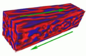
Figure 1: Spinodal decomposition under shear. Differently coloured regions denote the majority of the corresponding fluid. The arrows depict the movement of the sheared boundaries (movie available in online version).

3.2 Flow in porous media

Studying transport phenomena in porous media is of great interest in fields ranging from oil recovery and water purification to industrial processes like catalysis. In particular, the oilfield industry uses complex, non-Newtonian, multicomponent fluids (containing polymers, surfactants and/or colloids, brine, oil and/or gas), for processes like fracturing, well stimulation and enhanced oil recovery. The rheology and flow behaviour of these complex fluids in a rock is different from their bulk properties. It is therefore of considerable interest to be able to characterise and predict the flow of these fluids in porous media. From the point of view of a modelling approach, the treatment of complex fluids in three-dimensional complex geometries is an ambitious goal since the lattice has to be large enough to resolve individual structures. The advantage of lattice Boltzmann (or lattice gas) techniques is that complex geometries can be modelled with ease.

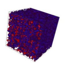
Figure 2: Rendering of $4.9\mu m$ resolution X-ray microtomographic data of a $512^{3}$ sample of Bentheimer sandstone. The pore space is shown in red, while the rock is represented in blue.

Synchrotron based X-ray microtomography (XMT) imaging techniques provide high resolution, three-dimensional digitised images of rock samples. By using the lattice Boltzmann approach in combination with these high resolution images of rocks, not only is it possible to compute macroscopic transport coefficients, such as the permeability of the medium, but information on local fields, such as velocity or fluid densities, can also be obtained at the pore scale, providing a detailed insight into local flow characterisation and supporting the interpretation of experimental measurements [Auzerais et al., 1996]. The XMT technique measures the linear attenuation coefficient from which the mineral concentration and composition of the rock can be computed. Morphological properties of the void space, such as pore size distribution and tortuosity, can be derived from the tomographic image of the rock volume, and the permeability and conductivity of the rock can be computed [Spanne et al., 1994]. The tomographic data are represented by a reflectivity greyscale value, where the linear size of each voxel is defined by the imaging resolution, which is usually on the order of microns. By introducing a threshold to discriminate between pore sites and rock sites, these images can be reduced to a binary (0’s and 1’s) representation of the rock geometry. Utilizing the lattice Boltzmann method, single phase or multiphase flow can then be described in these real porous media.

Lattice Boltzmann and lattice gas techniques have already been applied to study single and multiphase flow through three-dimensional microtomographic reconstruction of porous media. For example, Martys and Chen [Martys and Chen, 1996] and Ferréol and Rothman [Ferréol and Rothman, 1995] studied relative permeabilities of binary mixtures in Fontainebleau sandstone. These studies validated the model and the simulation techniques, but were limited to small lattice sizes, of the order of $64^{3}$. Simulating fluid flow in real rock samples allows us to compare simulation data with experimental results obtained on the same, or similar, pieces of rock. For a reasonable comparison, the size of the rock used in lattice Boltzmann simulations should be of the same order of magnitude as the system used in the experiments, or at least large enough to capture the rock’s topological features. The more inhomogeneous the rock, the larger the sample size needs to be in order to describe the correct pore distribution and connectivity. Another reason for needing to use large lattice sizes is the influence of boundary conditions and lattice resolution on the accuracy of the lattice Boltzmann method. It has been shown (see for example [He et al., 1997], [Chen and Doolen, 1998] and references therein) that the Bhatnagar-Gross-Krook (BGK) [Bhatnagar et al., 1954] approximation of the lattice Boltzmann equation which is commonly used causes so-called bounce-back boundaries to become inaccurate, resulting in effects such as the computed permeability being a function of the viscosity. This effect can be limited by lowering the viscosity and increasing the lattice resolution. To accurately describe hydrodynamic behaviour using lattice Boltzmann simulations, the Knudsen number, which represents the ratio of the mean free path of the fluid particles and the characteristic length scale of the system (such as the pore diameter), has to be small. If the pores are resolved with an insufficient number of lattice points, finite size effects arise, leading to an inaccurate description of the flow field. In practice, at least five to ten lattice sites are needed to resolve a single pore. Therefore, in order to be able to simulate realistic sample sizes, we need large lattices of the order of 512³.

Using LB3D, we are able to simulate drainage and imbibition processes in a $512^{3}$ subsample of Bentheimer sandstone X-ray tomographic data. The whole set of XMT data represented the image of a Bentheimer sample of cylindrical shape with diameter 4mm and length 3mm. The XMT data were obtained at the European Synchrotron Research Facility (Grenoble) at a resolution of $4.9\mu{\rm m}$, resulting in a data set of approximately 816x816x612 voxels. Figure 2 shows a snapshot of the $512^{3}$ subsystem. We compare simulated velocity distributions with experimentally obtained magnetic resonance imaging (MRI) data of oil and brine infiltration into saturated Bentheimer rock core [Sheppard et al., 2003]. The rock sample used in these MRI experiments had a diameter of 38 mm and was 70 mm long and was imaged with a resolution of 280 microns. The system simulated was smaller, but still of a similar order of magnitude and large enough to represent the rock geometry. On the other hand, the higher space resolution provided by the simulations allows a detailed characterisation of the flow field in the pore space, hence providing a useful tool to interpret the MRI experiments, for example in identifying regions of stagnant fluid. Figure 3 shows an example from a binary invasion study. A rock which is initially fully saturated with “water” (blue), is being invaded by “oil” (red) from the right side. The lattice size is $512^{3}$ and the forcing level is set to $g_{\rm accn}$ = 0.003. In figure 3, only the invading fluid component is shown, i.e. only areas where oil is the majority component are rendered. Periodic boundary conditions are applied, and fluid leaving the system on the left side is converted to oil before re-entering on the opposite side. After 5000 timesteps, the oil has invaded about one quarter of the system already and after 25000 timesteps only small regions of the rock pore space are still filled with water. After 30000 timesteps, the water component has been fully pushed out of the rock. This example only covers binary (oil/water) mixtures of Newtonian fluids, since this is a first and necessary step in the understanding of multiphase fluid flow in porous media [Harting et al., 2004b]. However, we are able to study the flow of binary immiscible fluids with an additional amphiphilic component in porous media and expect results to be presented elsewhere in the near future.

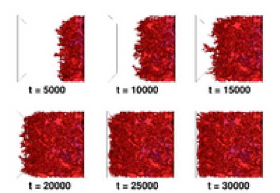
Figure 3: An originally fully fluid saturated rock is being invaded by another immiscible fluid using a body force $g_{\rm accn}$ = 0.003. The oil slowly pushes the other fluid component out of the rock pores until the rock is fully saturated by oil at $t$ = 30000. For better visability only the invading fluid is shown (movie available in online version).

3.3 The cubic gyroid mesophase

It was recently shown by González and Coveney[González-Segredo and Coveney, 2004b] that the dynamical self-assembly of a particular amphiphile mesophase, the gyroid, can be modelled using the lattice Boltzmann method. This mesophase was observed to form from a homogeneous mixture, without any external constraints imposed to bring about the gyroid geometry, which is an emergent effect of the mesoscopic fluid parameters. It is important to note that this method allows examination of the dynamics of mesophase formation, since most treatments to date have focussed on properties or mathematical description[Seddon and Templer, 1993, Schwarz and Gompper, 1999, Gandy and Klinowski, 2000, Große-Brauckmann, 1997] of the static equilibrium state. In addition to its biological importance, there have been recent attempts[Chan et al., 1999] to use self-assembling gyroids to construct nanoporous materials. During the gyroid self-assembly process, several small, separated gyroid-phase regions or domains may start to form, and then grow. Since the domains evolve independently, the independent gyroid regions will in general not be identical, and can differ in orientation, position, or unit cell size; grain-boundary defects arise between gyroid domains. Inside a domain, there may be dislocations, or line defects, corresponding to the termination of a plane of unit cells; there may also be localised non-gyroid regions, corresponding to defects due to contamination or inhomogeneities in the initial conditions. Understanding such defects is therefore important for our knowledge of the dynamics of surfactant systems, and crucial for an understanding of how best to produce mesophases experimentally and industrially.

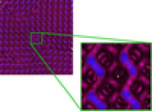
Figure 4: A volume rendered dataset of a 128³ system after 100000 simulation timesteps. Various gyroid domains have formed and the close-up shows the extremely regular, crystalline, gyroid structure within a domain (movies available in online version).

In small-scale simulations of the gyroid, the mesophase will evolve to fill the simulated region perfectly, without defects. As the lattice size grows, it becomes more probable that multiple gyroid domains will emerge independently, so that grain boundary defects are more likely to appear, and the time required for localized defects to diffuse across the lattice increases, making it more likely that defects will persist. Therefore, examination of the defect behaviour of surfactant mesophases requires the simulation of very large systems. Figure 4 shows an example of a 128³ system after 100000 simulation timesteps. Multiple gyroid domains have formed and the close-up shows the extremely regular, crystalline, gyroid structure within a domain. Figure 5 demonstrates some of the most interesting properties of the gyroid mesophase: two labyrinths mainly consisting of water and oil counterparts are enclosed by the gyroid minimal surface at which the surfactant molecules accumulate. The characteristic triple junctions can be seen clearly.

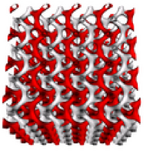
Figure 5: Structure of the two labyrinths enclosed by a gyroid minimal surface, showing the characteristic triple junctions.

The TeraGyroid experiment[Pickles et al., 2004, Blake et al., 2004] addressed a large scale problem of genuine scientific interest and showed how intercontinental grids permit the use of novel techniques in collaborative computational science, which can dramatically reduce the time to insight. TeraGyroid used computational steering over a Grid to study the self-assembly and dynamics of gyroid mesophases using the largest set of lattice Boltzmann simulations ever performed. Around the Supercomputing 2003 conference we were able to simulate gyroid formation and defect behaviour harnessing the compute power of a large fraction of the UK and US HPC facilities. Altogether we were able to use about 400000 CPU hours and generate two terabytes of simulation data.

Figure 6: In order to eliminate finite size effects from simulations, very large lattice sizes are needed. If one is interested in the statistical behaviour of defects, then the lattice size has to be increased even more, since otherwise only a limited number of defects can be found in the system. This figure shows a snapshot from what we believe to be the largest ternary lattice Boltzmann simulation ever performed, on a 1024³ lattice.

In order to make sure our simulations are virtually free of finite size effects, we simulated different system sizes from 64³ to 1024³, usually for about 100000 timesteps. In order to study the long term behaviour of the gyroid mesophase, some simulations have even run for one million timesteps. For 100000 timesteps we found that 256³ or even 128³ simulations do not suffer from finite size effects, but after very long simulation times we might even have to move to larger lattices. Even with the longest possible simulation times, we were not able to generate a “perfect” crystal. Instead, either differently orientated domains can still be found or individual defects are still moving around. It is of particular interest to study the exact behaviour of the defect movement, which can be done by gathering statistics of the simulation data by counting and tracking individual defects. Gathering useful statistics implies large numbers of measurements and therefore large lattices, which is the reason for the 512³ and 1024³ simulations performed. The memory requirements exceed the available resources on most supercomputers and limits us to a small number of machines. Also, it requires substantial amounts of CPU time to reach suffcient simulation times. In the case of the 1024³ system, 2048 CPUs of a recent Compaq Alpha cluster are only able to simulate about 100 simulation timesteps per hour. Running for 100000 timesteps would require more than two million CPU hours or 42 days and is therefore unfeasible. Also, handling the data files which are $4{\mathrm{GB}}$ each and checkpoint files which are $0.5{\mathrm{TB}}$ each is very awkward with the infrastructure available today. In order to be able to gain useful data from the large simulations, we first run a 128³ system with periodic boundary conditions, until it forms a gyroid. This system is then duplicated 512 times to produce a 1024³ gyroid system. In order to reduce effects introduced due to the periodic upscaling, we perturb the system and let it evolve. We anticipate that the unphysical effects introduced by the upscaling process will decay after a comparably small number of timesteps, thus resulting in a system that is comparable to one that started from a random mixture of fluids. This has to be justified by comparison with data obtained from test runs performed on smaller systems. Figure 6 shows a snapshot of a volume rendered dataset from the upscaled 1024³ system at 1000 timesteps after the upscaling process. The unphysical periodic structures introduced by the individual 128³ systems can still clearly be seen.

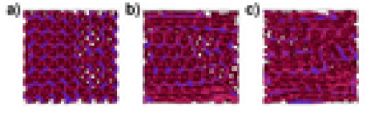
Figure 7: a sheared gyroid mesophase: a) before the onset of shear, b) at the onset of shear, c) after long shear times.

Currently, work is in progress to study the stability of the gyroid mesophase. We are interested in the influence of perturbation on a gyroid and the strength of the perturbation needed to break up a well developed mesophase. Similar studies are performed experimentally by applying constant or oscillatory shear. Here, we study the dependence of the gyroid stability on the shear rate, and expect to find evidence of the non-Newtonian properties of the fluid. An example from those studies can be seen in figure 7, which shows three snapshots of the same simulation. The first shows the liquid crystal before the onset of shear, the second only a few hundred timesteps after shear has been turned on and the third image demonstrates how the gyroid melts if the shear stress becomes too strong.

As seen before, simulation data from liquid crystal dynamics can be visualized using isosurfacing or volume rendering techniques. The human eye has a remarkable ability to easily distinguish between regions where the crystal structure is well developed and areas where it is not. However, manual analysis of large amounts of simulation data is not feasible. In the case of the TeraGyroid project, about two terabytes of data would have to be checked and catalogued manually. This task would keep an individual busy for years. Therefore, computational methods for defect detection and tracking are required. Developing algorithms to detect and track defects is a non-trivial task, however, since defects can occur within and between domains of varying shapes and sizes and over a wide variety of length and time scales. A standard method to analyse simulation data is the calculation of the three-dimensional structure function $S(\mathbf{k},t)\equiv\frac{1}{V}\left|\phi^{\prime}_{\mathbf{k}}(t)\right|^{2}$, where $V$ is the number of cites of the lattice, $\phi^{\prime}_{\mathbf{k}}(t)$ the Fourier transform of the fluctuations of the order parameter $\phi^{\prime}\equiv\phi-\left<\phi\right>$, and $\mathbf{k}$ is the wave vector [González-Segredo et al., 2003, González-Segredo and Coveney, 2004a]. $S(\mathbf{k},t)$ can easily be calculated, but only gives general information about the crystal development [Hajduk et al., 1994, Laurer et al., 1997, González-Segredo and Coveney, 2004b]. It does not allow one to detect where the defects are located or how many there are, nor does it furnish access to information about the number of differently oriented gyroid domains. $S(\mathbf{k},t)$ is given for a 128³ system at timesteps $t$=10000, 100000, and 700000 in figure 8. We simulate for one million timesteps – more than an order of magnitude longer than any other LB3D simulation performed before the TeraGyroid [TeraGyroid, 2003] project. The initial condition of the simulation is a random mixture with maximum densities of 0.7 for the immiscible fluids and 0.6 for surfactant. The coupling constant $g_{ss}$ is set to -0.0045 and the coupling between surfactant and the other fluids is set to $g_{cs}$=-0.006. In order to compare our data to experimentally obtained SAXS data [Hajduk et al., 1994], we sum the structure factor in the $x$-direction; $X_{max}$ denotes the value of the largest peak normalised by the number of lattice sites in the direction of summation (128 in this case) [Harting et al., 2004a]. Gyroid assembly is evident due to the eight peaks of the structure factor which become higher with ongoing simulation time. At $t$=700000, $X_{max}$ reaches 197.00 and most of the previously existing domains have merged into a single one. Only a few defects are left of which two can be spotted visually at the right corner of the volume rendered visualisation and the centre of the top surface (denoted by the white arrows).

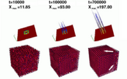
Figure 8: Three-dimensional structure factor of the order parameter at timesteps $t$=10000, 100000, and 700000, lattice size 128³ and simulation parameters as given in the text. For comparability with SAXS experimental data, we display the total structure factor in the $x$-direction $X$=$\sum_{k_{x}}S(\mathbf{k},t)$. $X_{max}$ denotes the value of the largest peak divided by the number of lattice sites in the direction of summation (128 in this case). The lower half of the figure shows volume rendered visualizations of the corresponding order parameters and the white arrows are a guide for the eye to spot some defective areas at the top surface and the right corner at $t$=700000.

The structure factor analysis does not provide any information about the size, position or number of individual defects in the system. Therefore, we developed more advanced algorithms for the detection and tracking of defects. As a first order approach, the data to be analyzed can be reduced by cutting the three-dimensional data sets into slabs and projecting them onto a two-dimensional plane. By using a raytracing algorithm for the projection, we obtain regular patterns in areas where the gyroid is perfectly developed and solid planes in defective areas. We developed two algorithms which use the projection data to separate the defective areas from the perfect crystal. The first approach is based on a generic pattern recognition algorithm and should work with all liquid crystals that form a regular pattern, while the second has been developed with our particular problem in mind and is not known to work with systems other than the gyroid mesophase. However, it is about an order of magnitude faster and the general principles underlying it should be applicable to different systems as well. The first approach is based on the regularity or periodicity of patterns and was developed by Chetverikov and Hanbury in 2001 [Chetverikov and Hanbury, 2002] who applied it to patterns from the textile industry. It is assumed that defect-free patterns are homogeneous and show some periodicity. The algorithm searches for areas which are significantly less regular (i.e. aperiodic) than the bulk of the dataset by computing regularity features for a set of windows and identifying defects as outliers. The regularity is quantified by computing the periodicity of the normalised autocorrelation function in polar coordinates. In short, for every window a regularity value is computed. If this value differs by more than a defined threshold value from the median of all window regularity values, the area is accordingly classified as a defect. For a more detailed description of the algorithm see [Chetverikov and Hanbury, 2002, Chetverikov, 2000, Harting et al., 2004a]. The second approach encapsulates knowledge about the patterns produced by regular and defect regions. As a consequence, it is an order of magnitude faster than the pattern recognition code. For each slab image, the algorithm creates a regular mesh in areas where the gyroid structure is well developed, and an irregular mesh in defective areas. The regions of regular mesh are discarded, leaving only mesh that describes the perimeters of defect regions. A flood-fill algorithm is applied to these datasets to locate distinct defect regions. The output data of both detection algorithms for all two-dimensional projections of a three-dimensional dataset can be used to reconstruct three-dimensional volume data that only consists of defect regions. Figure 9 shows reconstructed datasets at $t$=340000, 500000 and 999000 which have been detected using the pattern recognition approach. However, the results obtained from the mesh generator are similar. Even at $t$=340000 a very large region of the system has not yet formed a well defined gyroid phase. 160000 timesteps later, the main defects are pillar shaped ones at the centre and at the corners of the visualised systems. Due to the periodic boundary conditions, the corner defects are connected and should be regarded as a single one. As can be seen from the analysis at $t$=999000, defects in the gyroid mesophase are very stable in size as well as in their position.

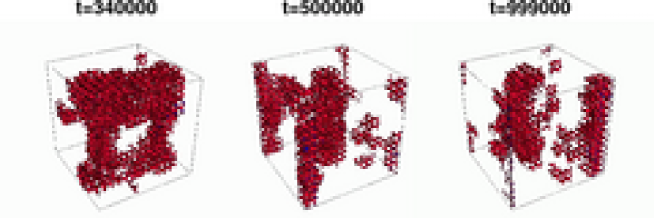
Figure 9: Volume rendered visualization of the order parameter at t=340000, 500000, 999000. Only the defects are shown as they have been isolated from the full datasets using the pattern recognition algorithm (movie available in onine version).

The pattern recognition algorithm is less efficient than mesh generation. However, it is not limited to simulations of gyroid mesophases and more robust with regrd to small fluctuations of the dataset. In the gyroid case, it is more efficient to use the results from the mesh generator to select a smaller number of datasets for post-processing using the pattern recognition algorithm since the computational effort involved in the pattern recognition can be substantial. For a more detailed description of the algorithms see [Harting et al., 2004a]. Currently, we are working on more geometrically based algorithms to efficiently detect defects and results will be published elsewhere in the near future.

4 Conclusions

During the last two years, we have worked on various scientific projects using our lattice Boltzmann code LB3D. All of these projects reached the limits of the HPC resources available to us today. However, without the benefits obtained from software development within the RealityGrid project, none of these projects would have been possible at all. These improvements include the steering facilities, code optimizations, IO optimizations as well as the platform independent checkpointing and migration routines which have been contributed by various people within the project. Without the lightweight Grid Service Container OGSI: ​​​​:Lite [McKeown, 2003] projects like the TeraGyroid experiment would not have been possible since existing middleware toolkits such as Globus are rather heavyweight, requiring substantial effort and local tuning on the part of systems administrators to install and maintain. This effort cannot be expected from the average scientist who is planning to use a computational grid[Chin and Coveney, 2004]. The simulation pipeline requires simulation, visualization, and storage facilities to be available simultaneously, at times when their human operators can reasonably expected to be around. This is often dealt with by manual reservation of resources by systems administrators, but the ideal solution would involve automated advance reservation and co-allocation procedures. The most exciting project involving RealityGrid during the last two years was the TeraGyroid experiment. Hundreds of individuals have worked together to build a transcontinental grid not only as a demonstrator for the grid techniques available today, but to perform a scientific project. Since we would not have been able to gain as many new results from the simulations performed during that period without the active use of grid technologies, we have shown that the advent of computational grids will be of great benefit for computational scientists.

References

- Auzerais et al., 1996 Auzerais, F. M., Dunsmuir, J., Ferreol, B. B., Martys, N., Olson, J., Ramakrishnan, T., Rothman, D., and Schwartz, L.: 1996, Geophys. Research Lett. 23(7), 705
- Benzi et al., 1992 Benzi, R., Succi, S., and Vergassola, M.: 1992, Phys. Rep. 222(3), 145
- Berman et al., 2003 Berman, F., Fox, G., and Hey, T.: 2003, Grid Computing: Making The Global Infrastructure a Reality, John Wiley and Sons
- Bhatnagar et al., 1954 Bhatnagar, P. L., Gross, E. P., and Krook, M.: 1954, Phys. Rev. 94(3), 511
- Blake et al., 2004 Blake, R., Coveney, P., Clarke, P., and Pickles, S.: 2004, EPSRC final report
- Boghosian et al., 2000 Boghosian, B. M., Coveney, P. V., and Love, P. J.: 2000, Proc. R. Soc. Lond. A 456, 1431
- Brooke et al., 2003 Brooke, J. M., Coveney, P. V., Harting, J., Jha, S., Pickles, S. M., Pinning, R. L., and Porter, A. R.: 2003, in Proceedings of the UK e-Science All Hands Meeting, September 2-4
- Chan et al., 1999 Chan, V. Z. H., Hoffman, J., Lee, V. Y., Iatrou, H., Avgeropoulos, A., Hadjichristidis, N., Miller, R. D., and Thomas, E. L.: 1999, Science 286(5445), 1716
- Chapman and Cowling, 1952 Chapman, S. and Cowling, T. G.: 1952, The Mathematical Theory of Non-uniform Gases, Cambridge University Press, second edition
- Chen et al., 2000 Chen, H., Boghosian, B. M., Coveney, P. V., and Nekovee, M.: 2000, Proc. R. Soc. Lond. A 456, 2043
- Chen and Doolen, 1998 Chen, S. and Doolen, G. D.: 1998, Annu. Rev. Fluid Mech. 30, 329
- Chetverikov, 2000 Chetverikov, D.: 2000, Image and Vision Computing 18, 975
- Chetverikov and Hanbury, 2002 Chetverikov, D. and Hanbury, A.: 2002, Pattern Recognition 35, 203, An online demo of the algorithm is available at http://aramis.ipan.sztaki.hu/strucdef/strucdef.html
- Chin and Coveney, 2002 Chin, J. and Coveney, P. V.: 2002, Phys. Rev. E 66(016303)
- Chin and Coveney, 2004 Chin, J. and Coveney, P. V.: 2004, Towards tractable toolkits for the Grid: a plea for lightweight, usable middleware
- Chin et al., 2003 Chin, J., Harting, J., Jha, S., Coveney, P. V., Porter, A. R., and Pickles, S. M.: 2003, Contemporary Physics 44(5), 417
- Czeslik and Winter, 2002 Czeslik, C. and Winter, R.: 2002, J. Mol. Liq. 98, 283
- Delgado-Buscalioni and Coveney, 2003 Delgado-Buscalioni, R. and Coveney, P. V.: 2003, Phys. Rev. E 67(046704)
- Espaol and Warren, 1995 Espaol, P. and Warren, P.: 1995, Europhys. Lett. 30(4), 191
- Faber, 1995 Faber, T. E.: 1995, Fluid Dynamics for Physicists, Cambridge University Press
- Ferréol and Rothman, 1995 Ferréol, B. and Rothman, D. H.: 1995, Transport in porous media 20, 3
- Flekkøy et al., 2000 Flekkøy, E. G., Coveney, P. V., and Fabritiis, G. D.: 2000, Phys. Rev. E 62(2), 2140
- Foster and Kesselman, 1999 Foster, I. and Kesselman, C.: 1999, in I. Foster and C. Kesselman (eds.), The Grid: Blueprint for a New Computing Infrastructure, pp 15–25, Morgan Kaufmann
- Frisch et al., 1986 Frisch, U., Hasslacher, B., and Pomeau, Y.: 1986, Phys. Rev. Lett. 56(14), 1505
- Gandy and Klinowski, 2000 Gandy, P. J. F. and Klinowski, J.: 2000, Chem. Phys. Lett. 321(5), 363
- Garcia et al., 1999 Garcia, A. L., Bell, J. B., Crutchfield, W. Y., and Alter, B. J.: 1999, J. Comp. Phys. 154(1), 134
- González-Segredo and Coveney, 2004a González-Segredo, N. and Coveney, P. V.: 2004a, Phys. Rev. E 69, 061501
- González-Segredo and Coveney, 2004b González-Segredo, N. and Coveney, P. V.: 2004b, Europhys. Lett. 65(6), 795
- González-Segredo et al., 2003 González-Segredo, N., Nekovee, M., and Coveney, P. V.: 2003, Phys. Rev. E 67(046304)
- Große-Brauckmann, 1997 Große-Brauckmann, K.: 1997, Exp. Math. 6(1), 33
- Hajduk et al., 1994 Hajduk, D. A., Harper, P. E., Gruner, S. M., Honeker, C. C., Kim, G., and Thomas, E. L.: 1994, Macromolecules 27, 4063
- Harting et al., 2004a Harting, J., Harvey, M. J., Chin, J., and .V.Coveney, P.: 2004a, Detection and tracking of defects in the gyroid mesophase, Accepted for publication in Comp.Phys.Comm.
- Harting et al., 2004b Harting, J., Venturoli, M., and Coveney, P. V.: 2004b, Phil. Trans. R. Soc. Lond. A 362, 1703
- Hashimoto et al., 2000 Hashimoto, Y., Chen, Y., and Ohashi, H.: 2000, Comp. Phys. Comm. 129(1–3), 56
- HDF5, 2003 HDF5: 2003, HDF5 – a general purpose library and file format for storing scientific data, http://hdf.ncsa.uiuc.edu/HDF5
- He et al., 1997 He, X., Q. Zou, L. L., and Dembo, M.: 1997, J. Stat. Phys. 87(115),
- Higuera and Jiménez, 1989 Higuera, F. J. and Jiménez, J.: 1989, Europhys. Lett. 9(7), 663
- Higuera et al., 1989 Higuera, P. J., Succi, S., and Benzi, R.: 1989, Europhys. Lett. 9(4), 345
- Hoogerbrugge and Koelman, 1992 Hoogerbrugge, P. J. and Koelman, J. M. V. A.: 1992, Europhys. Lett. 19(3), 155
- Jury et al., 1999 Jury, S., Bladon, P., Cates, M., Krishna, S., Hagen, M., Ruddock, N., and Warren, P.: 1999, Phys. Chem. Chem. Phys. 1, 2051
- Lamura et al., 1999 Lamura, A., Gonnella, G., and Yeomans, J. M.: 1999, Europhys. Lett. 45(3), 314
- Landh, 1995 Landh, T.: 1995, FEBS Lett. 369(1), 13
- Laurer et al., 1997 Laurer, J. H., Hajduk, D. A., Fung, J. C., Sedat, J. W., Smith, S. F., Gruner, S. M., Agard, D. A., and Spontak, R. J.: 1997, Macromolecules 30, 3938
- Lees and Edwards, 1972 Lees, A. and Edwards, S.: 1972, J. Phys. C. 5(15), 1921
- Liboff, 1990 Liboff, R. L.: 1990, Kinetic Theory: Classical, Quantum, and Relativistic Descriptions, Prentice-Hall
- Love, 2002 Love, P. J.: 2002, Phil. Trans. R. Soc. Lond. A 360, 345
- Love et al., 2003 Love, P. J., Nekovee, M., Coveney, P. V., Chin, J., González-Segredo, N., and Martin, J. M. R.: 2003, Comp. Phys. Comm. 153, 340
- Malevanets and Kapral, 1998 Malevanets, A. and Kapral, R.: 1998, Europhys. Lett. 44(5), 552
- Malevanets and Yeomans, 2000 Malevanets, A. and Yeomans, J. M.: 2000, Europhys. Lett. 52(2), 231
- Martys and Chen, 1996 Martys, N. S. and Chen, H.: 1996, Phys. Rev. E 53(1), 743
- Martys and Douglas, 2001 Martys, N. S. and Douglas, J. F.: 2001, Phys. Rev. E 63, 031205
- McKeown, 2003 McKeown, M.: 2003, OGSI::Lite - an OGSI implementation in Perl
- McNamara and Zanetti, 1988 McNamara, G. R. and Zanetti, G.: 1988, Phys. Rev. Lett. 61(20), 2332
- Nekovee and Coveney, 2001a Nekovee, M. and Coveney, P.: 2001a, J. Am. Chem. Soc. 123(49), 12380
- Nekovee and Coveney, 2001b Nekovee, M. and Coveney, P. V.: 2001b, J. Am. Chem. Soc. 123(49), 12380
- Pickles et al., 2004 Pickles, S. M., Blake, R. J., Boghosian, B. M., Brooke, J. M., Chin, J., Clarke, P. E. L., Coveney, P. V., González-Segredo, N., Haines, R., Harting, J., Harvey, M., Jha, S., Jones, M. A. S., McKeown, M., Pinning, R. K., Porter, A. R., Roy, K., and Riding, M.: 2004, Proceedings of the Workshop on Case Studies on Grid Applications at GGF 10
- Rivet and Boon, 2001 Rivet, J.-P. and Boon, J. P.: 2001, Lattice Gas Hydrodynamics, Cambridge University Press
- Rothman and Keller, 1988 Rothman, D. H. and Keller, J. M.: 1988, J. Stat. Phys. 52(3–4), 1119
- Sakai et al., 2000 Sakai, T., Chen, Y., and Ohashi, H.: 2000, Comp. Phys. Comm. 129(1–3), 75
- Schroeder et al., 2003 Schroeder, W., Martin, K., and Lorensen, B.: 2003, The Visualization Toolkit: An Object Oriented Approach to 3D Graphics, Kitware, Inc., 3rd edition
- Schwarz and Gompper, 1999 Schwarz, U. S. and Gompper, G.: 1999, Phys. Rev. E 59(5), 5528
- Seddon and Templer, 1993 Seddon, J. M. and Templer, R. H.: 1993, Phil. Trans.: Phys. Sci. Eng. 344(1672), 377
- Seddon and Templer, 1995 Seddon, J. M. and Templer, R. H.: 1995, Polymorphism of Lipid-Water Systems, Chapt. 3, pp 97–160, Elsevier Science B. V.
- Shan and Chen, 1993 Shan, X. and Chen, H.: 1993, Phys. Rev. E 47(3), 1815
- Shan and Chen, 1994 Shan, X. and Chen, H.: 1994, Phys. Rev. E 49(4), 2941
- Shefelbine et al., 1999 Shefelbine, T. A., Vigild, M. E., Matsen, M. W., Hajduk, D. A., Hillmyer, M. A., Cussler, E. L., and Bates, F. S.: 1999, J. Am. Chem. Soc. 121(37), 8457
- Sheppard et al., 2003 Sheppard, S., Sederman, A., Verganelakis, D., Johns, M., Mantle, M., and Gladden, L.: 2003, Probing Pore Scale Velocity Fields During Fluid Flow in Porous Media: Displacement Propagators of non-Newtonian Fluids in Sedimentary Rocks, Technical report, Schlumberger Cambridge Research, Department of Chemical Engennering, University of Cambridge UK, Poster presentation at International Conference on magnetic Resonance Microscopy 20-25 September 2003
- Spanne et al., 1994 Spanne, P., Thovert, J. F., Jacquin, C. J., Lindquist, W. B., Jones, K. W., and Adler, P. M.: 1994, Phys. Rev. Lett. 73(14), 2001
- Succi, 2001 Succi, S.: 2001, The Lattice Boltzmann Equation for Fluid Dynamics and Beyond, Oxford University Press
- TeraGyroid, 2003 TeraGyroid: 2003, The TeraGyroid project: http://www.RealityGrid.org/TeraGyroid.html
- Wagner and Pagonabarraga, 2002 Wagner, A. and Pagonabarraga, I.: 2002, J. Stat. Phys. 107, 521, cond-mat/0103218]
- Wagner and Yeomans, 1999 Wagner, A. J. and Yeomans, J. M.: 1999, Phys. Rev. E 59(4), 4366