Enhancing Histograms by Tree-Like Bucket Indices

Abstract

Histograms are used to summarize the contents of relations into a number of buckets for the estimation of query result sizes. Several techniques (e.g., MaxDiff and V-Optimal) have been proposed in the past for determining bucket boundaries which provide accurate estimations. However, while search strategies for optimal bucket boundaries are rather sophisticated, no much attention has been paid for estimating queries inside buckets and all of the above techniques adopt naive methods for such an estimation. This paper focuses on the problem of improving the estimation inside a bucket once its boundaries have been fixed. The proposed technique is based on the addition, to each bucket, of 32-bit additional information (organized into a 4-level tree index), storing approximate cumulative frequencies at 7 internal intervals of the bucket. Both theoretical analysis and experimental results show that, among a number of alternative ways to organize the additional information, the 4-level tree index provides the best frequency estimation inside a bucket. The index is later added to two well-known histograms, MaxDiff and V-Optimal, obtaining the non-obvious result that despite the spatial cost of 4LT which reduces the number of allowed buckets once the storage space has been fixed, the original methods are strongly improved in terms of accuracy.

1 Introduction

A histogram is a lossy compression technique used for representing efficiently a relation. It is based on the partition of one of the relation attributes into buckets and the storage, for each of them, of a few summary information in place of the detailed one. Among others, some important examples of application domains of histograms are the estimation of query selectivity IoPo95 ; Jagadish98Optimal ; Poosala96Improved ; Ja*01 ; Wu03Using , temporal databases, where histograms are used for improving the join processing Sitzmann00Improving , statistical databases, where histograms represent a method for approximating probability distributions Malvestuto93Universal . Recently, histograms have received a new deal of interest, mainly because they can be effectively used for approximating query answering in order to reduce the query response time in on-line decision support systems and OLAP Poosala99Approx , as well as the problem of reconstructing original data from aggregate information BuFuSa01 and, finally, in the context of Data Streams Guha01Data ; Babcock02Models ; Datar02Maintaining ; Guha02Histogramming .

For a given storage space reduction, the problem of determining the best histogram is crucial. Indeed, different partitions lead to dramatically different errors in reconstructing the original data distribution, especially for skewed data. To better explain the problem, consider a typical case of recovering original data from a histogram: the evaluation of range queries. Think to a histogram defined on the attribute $X$ of a relation $R$ as a set of non-overlapping intervals of $X$ covering all values assumed by $X$ in $R$. To each of these intervals, say $B$, the number of occurrences (called frequency) in $R$, having the value of $X$ belonging to the interval $B$, is associated (and included into a data structure called bucket). A range query, defined on an interval $Q$ of $X$, evaluates the number of occurrences in $R$ with value of $X$ in $Q$. Thus, buckets embed a set of pre-computed disjoint range queries capable of covering the whole active domain of $X$ in $R$ (with active here we mean attribute values actually appearing in $R$). As a consequence, the histogram does not give, in general, the possibility of evaluating exactly a range query not corresponding to one of the pre-computed embedded queries. In other words, while the contribution to the answer coming from the sub-ranges coinciding with entire buckets can be returned exactly, the contribution coming from the sub-ranges which partially overlap buckets can be only estimated, since the actual data distribution inside the buckets is not available.

It turns out that it is convenient to define the boundaries of buckets in such a way that the estimation error of the non-precomputed range queries is minimized (e.g., by avoiding that large frequency differences arise inside a bucket). In other words, among all possible sets of pre-computed range queries, we find the set which guarantees the best estimation of the other (non-precomputed) queries, once a technique for estimating such queries is defined. This issue is being investigated since some decades, and a large number of techniques for arranging histograms have been proposed Cri81 ; Cri84 ; IoPo95 ; Jagadish98Optimal ; Poosala96Improved ; DonIoa00 ; Ja*01 .

All these techniques adopt simple methods for estimating non-precomputed queries (actually, their portions partially overlapping buckets). The most significant approaches are the continuous value assumption (often denoted in this paper by CVA) Sac79 , where the estimation is made by linear interpolation on the whole domain of the bucket, and the uniform spread assumption (denoted by USA) Poosala96Improved , which assumes that values are located at equal distance from each other so that the overall frequency sum can be equally distributed among them.

An interesting problem is understanding whether, by exploiting information typically contained in histogram buckets, and possibly adding a few summary information, the frequency estimation inside buckets, and then, the histogram accuracy, can be improved. This paper focuses on this problem. Starting from the consideration of limits of CVA and USA studied in BuFuSa01 , we propose to use some additional storage space in order to describe the distribution inside a bucket in an approximate yet very effective way.

The first step is studying how to use these 32 additional bits in order to maximize benefits in terms of accuracy. Our analysis shows that the trivial technique of partitioning the bucket into 8 equal-size parts and encoding each corresponding sum by 4 bits, leads to high scaling errors since it is needed to represent each sum as a fraction of the overall sum of the bucket. Our proposal then relies on the idea of storing partial sums internal to the bucket in a hierarchical fashion, using a tree-like index (occupying 32 bits). This way, the sum contained in a given tree node, can be represented as a fraction of the sum contained in the parent node, which is a value (reasonably) smaller than the overall sum of the bucket. It turns out that the encoding length may decrease as the level of the tree increases. The benefits we expect by applying this approach concern the scaling error. But a crucial point is to decide how to arrange the tree, that is, how far going down in depth with the index. Of course, the higher the resolution, the larger the number of embedded precomputed range queries (internal to the buckets) is. Hence, we expect better accuracy as the resolution increases. However, increasing resolution reduces the number of bits available for encoding nodes, and, thus, amplifies scaling errors. We study the above trade-off by considering the two possible (from a practical point of view) tree-indices with 32 bits, which we call 3LT and 4LT, with depth 3 and 4, respectively. The analysis leads to the conclusion that the 4LT-index represents the best solution.

The next step is then understanding whether this improvement of accuracy for the estimation inside buckets can really give benefits in terms of accuracy of a histogram arranged by one of the existing techniques. This problem is not straightforward: think, to mention the most evident aspect, that 4LT buckets use 32 bits more than CVA ones, and, then, for a fixed storage space, allows a smaller number of buckets. The last part of this paper is thus devoted to evaluate the effects of the combination of the 4LT technique with existing methods for building histograms. Through a deep experimental comparative analysis conducted, for a fixed storage space, over several data sets, both synthetic and real-life, we show that 4LT improves significantly the accuracy of the considered histograms. Therefore this paper, beside giving the specific contribution of proposing a technique (i.e., the 4LT) for estimating accurately range queries internal to buckets, proves the more general result that going beyond classical techniques (i.e., CVA and USA) for the estimation inside buckets may give concrete improvements of histogram accuracy.

It is worth noting that the choice of MaxDiff and V-Optimal histograms for testing our method does not limit the generality of the 4LT index, which is applicable to every bucket-based histogram. Nevertheless, it is not limited the validity of our comparison, since MaxDiff and V-Optimal, despite their non-young age, are still considered in this scientific community as point of references due to their accuracy Ioannidis03History .

The paper is organized as follows. In Section 2, we introduce some preliminary definitions. The comparison, both experimental and theoretical, among a number of techniques including our tree-based methods (3LT and 4LT) for estimating range queries inside a bucket is reported in Section 3. Therein, 3LT and 4LT are also presented. From this analysis it results that 4LT has the best performances in terms of accuracy. Thus, 4LT can be combined to every bucked-based histogram for increasing its accuracy. Section 4 presents a large set of experiments, conducted by applying 4LT to two, well-known methods, MaxDiff and V-Optimal Poosala96Improved . Results show high improvements in the estimation of range queries w.r.t. to the original methods — of course, the comparisons are made at parity of storage consumption so that the revised methods use less buckets to compensate the additional storage for the 4LT indices. The 4LT technique provides good results also when combined with the very simple method EquiSplit, which consists in dividing the histogram value domain into buckets of the same size so that the bucket boundaries need not to be stored, thus obtaining a very high number of buckets at the same compression rate. We draw our conclusions in Section 5.

2 Basic Definitions

Given a relation $R$ and an attribute $X$ of $R$, a histogram for $R$ on $X$ is constructed as follows. Let ${{\cal U}}=\{u_{1},...,u_{m}\}$ be the set of all possible values (the domain) of $X$ and let $u_{i}<u_{i+1}$, for each $i$, $1\leq i<m$. The frequency set for $X$ is the set ${{\cal F}}=\{f(u_{1}),...,f(u_{m})\}$ such that for each $i$, $1\leq i\leq m$, $f(u_{i})$ is the number of occurrences of the attribute value $u_{i}$ in the relation $R$. The cumulative frequency set ${{\cal S}}=\{s_{1},...,s_{m}\}$ contains the value $s_{i}=\sum_{j=1}^{i}f(u_{j})$ for each attribute value $u_{i}$. The value set $V=$ $\{u_{i}\in{{\cal U}}\ |\ f(u_{i})>0\}$ is the active domain of $X$ in $R$ as it consists of all attribute values actually occurring in the relation $R$ (non-null values). Given any $u_{i}$ in $V$, the spread $d_{i}$ of $u_{i}\in V$ for $1\leq i<n$ is defined as 1 if $u_{i}$ is the last non-null value or otherwise as the difference $u_{j}-u_{i}$, where $u_{j}$ is the first non-null value for which $u_{j}>u_{i}$ (i.e., $d_{i}$ is the distance from $u_{i}$ to the next non-null value).

A bucket $B$ for $R$ on $X$ is a 4-tuple $\langle inf,sup,t,c\rangle$, where $u_{inf}$ and $u_{sup}$, $1\leq inf\leq sup\leq m$, are the boundaries of the domain range pertaining to the bucket, $t$ is the number of non-null values occurring in the range, and $c=\sum_{i=inf}^{sup}f(u_{i})$ is the sum of frequencies of all values in the range. We say that the bucket $B$ is 1-biased if $u_{sup}$ is not null; if also $u_{inf}$ is not null, then we say that $B$ is 2-biased.

A histogram $H$ for $R$ on $X$ is a $h$-tuple $\langle B_{1},B_{2},...,B_{h}\rangle$ of buckets such that: (1) for each $1\leq i<h$, the upper bound of $B_{i}$ precedes the lower bound of $B_{i+1}$ and (2) $u\in V$ implies $u\in B_{i}$, for some $i$, $1\leq i\leq h$. Condition (1) guarantees that buckets do not overlap each other, and condition (2) enforces that every non-null value be hosted by some bucket. Classically, histograms have 2-biased buckets; sometime, for storage optimizations, 2-biased buckets are made 1-biased by replacing the lower bound of each bucket with the successive in the domain of the upper bound of the preceding bucket.

A classical problem on histograms is: given a histogram $H$ and a (range) query of the form $u_{j}\leq X\leq u_{i}$, $1\leq j\leq i\leq m$, estimate the overall frequency $\sum_{k=j}^{i}f(i)$ in the range from $u_{j}$ to $u_{i}$.

3 Estimation Inside a Bucket

In this section we deeply investigate the problem of frequency estimation inside buckets. First of all, we present the classical two techniques (CVA and USA), discuss their limitations and propose some simple alternatives. Then we introduce a novel technique which is based on a 4-level tree index storing approximate representations of the partial sums of 7 fixed bucket intervals. Later we evaluate the accuracy of the various techniques by performing both a theoretical analysis of errors and a number of experiments on some typical sample distributions.

3.1 Notations and Problem Formulation

Let $B=\langle inf,sup,t,c\rangle$ be a bucket on an attribute $X$ of a relation $R$. Without loss of generality, we assume that $inf=1$ and $sup=b$ so that we can represent the frequency set inside the bucket as a vector $F$ with indexes ranging from $1$ to $b$ (frequency vector of $B$). Similarly, the cumulative frequencies are represented by a vector $S$ with indexes from $1$ to $b$ (cumulative frequency vector of $B$). Hence, for each $i$, $1\leq i\leq b$, $F[i]\geq 0$ is the frequency of the value $u_{i}$ while $S[i]=$ $\sum_{j=1}^{i}F[j]$ is the cumulative frequency. Then $c=S[b]$ is the sum of all frequencies in the bucket; moreover, for notation convenience, we assume that $S[0]=0$.

The problem of the estimation inside a bucket can be formulated as follows: given any pair $i,j$, $1\leq i\leq j\leq b$, such that $d=j-i+1<b$, estimate the range query $S[j]-S[i-1]=$ $\sum_{k=i}^{j}F[k]$. We focus our attention on the basic problem of estimating $S[d]$ (then by assuming $i=1$).

We introduce now the following notation. Given $1\leq i\leq j\leq 8$, we denote by $\delta_{i/j}$ the sum $\sum_{i=x}^{y}F[i]$, where $x=1+\lceil\frac{b}{j}\cdot(i-1)\rceil$ and $y=\lceil\frac{b}{j}\cdot i\rceil$. $\delta_{i/j}$ represents the frequency sum of the $i-$th elements of the partition of $B$ into $j$ equal size sub-ranges. Thus, the frequency sum for a bucket is $\delta_{1/1}$; the frequency sums for two halves are $\delta_{1/2}$ and $\delta_{2/2}$; the frequency sums for the 4 quarters are $\delta_{i/4}$, $1\leq i\leq 4$; the frequency sums for the 8 eighths are $\delta_{i/8}$, $1\leq i\leq 8$, and so on.

3.2 Estimation Techniques

Next we illustrate the existing approximation techniques and discuss some additional simple approaches.

Continuous Value Assumption (CVA). The estimation of $S[d]$ is computed as $\widetilde{S}[d]=\frac{d}{b}\cdot c$. In words, the partial contribution of a bucket to a range query result is estimated by linear interpolation. As pointed out in Buccafurri99Compressed ; BuFuSa01 , the above estimation coincides with the expected value of the $S[d]$ when it is considered a random variable over the population of all frequency distributions in the bucket for which the overall cumulative frequency is $c$. Uniform Spread Assumption (USA). The estimation of $S[d]$ is given by $\widetilde{S}[d]=\left(1+\frac{(t-1)\cdot(d-1)}{(b-1)}\right)\cdot\frac{c}{t}$, where $t$ is the number of non-null attribute values in the bucket. The uniform spread assumption assumes that such values are distributed at equal distance from each other and the overall frequency sum is equally distributed among them. Obviously, in this case the information $t$ is necessary. We stress that, as discussed in BuFuSa01 , this estimation is not supported by any unbiased probabilistic model so the assumption is rather arbitrary.

1-Biased Estimation (1b). The possibly available information on the number $t$ of non-null elements cannot be exploited in the estimation unless some further information on the frequency distribution is either available or assumed (as for the USA estimation). We next show how to exploit the fact that a bucket is often 1-biased (i.e., $u_{b}$ is not null) using the probabilistic approach proposed in BuFuSa01 . This approach assumes that the query is a random variable on the population of all 1-biased frequency distributions having $c$ as overall cumulative frequency. The estimation of the range query $S[d]$ for a 1-biased bucket is given by $\widetilde{S}[d]=\frac{d}{b-1}\cdot\frac{t-1}{t}\cdot c$.

2-Split Estimation (2s). We split the bucket into two parts of the same size and store the cumulative frequency of the first part, say $\delta_{1/2}=S[b/2]$ — we therefore need additional storage space (typically 32 bits). We call this method 2-split or $2s$ for short. Following this approach, the estimation of the range query $S[d]$ is given by $2\cdot\frac{d}{b}\cdot\delta_{1/2}$ if $d\leq\frac{b}{2}$, $\delta_{1/2}+2\cdot\frac{d-b}{b}\cdot(c-\delta_{1/2})$, otherwise. Thus we use the CVA techniques for each of the two halves of the bucket.

4-Split Estimation (4s). We split the bucket into 4 parts of the same size (quarts) and store the approximate values of the cumulative frequency of the each part $\delta_{i/4}$, $1\leq i\leq 4$. In case the additional available space is 32 bits, we use 8 bits for each approximate value, which is therefore computed as $\tilde{\delta}_{i/4}=\langle\frac{\delta_{i/4}}{c}\times(2^{8}-1)\rangle$, where $\langle x\rangle$ stands for $round(x)$. The frequency sum for an interval $d$ is estimated by adding the approximate values of all first quarts that are fully contained in the interval plus the CVA estimation of the portion of the last eighth that partially overlaps the interval. Obviously, in order to reduce the approximation error, in case $d>b/2$, it is convenient to derive the approximate value from the estimation of the cumulative frequency in the complementary interval from $d+1$ to $b$.

8-Split Estimation (8s). It is analogous to the 4-Split Estimation. The only difference is that the bucket is divided into 8 parts (eighths) and, for each of them, we use 4 bits for storing the cumulative frequency. Thus, the approximate value of the $i$-th eight ($1\leq i\leq 4$) , is computed as $\tilde{\delta}_{i/8}=\langle\frac{\delta_{i/8}}{c}\times(2^{4}-1)\rangle$, where $\langle x\rangle$ stands for $round(x)$.

3.3 The Tree Indices for Bucket Frequency Estimation

We now propose to use 32 bits as sophisticated tree-indices for providing an approximate description of the cumulative frequencies in the bucket — this index can be easily extended also to the case that more bits are available. To this end, we store the approximate value of the cumulative frequency in a suitable number of intervals inside the bucket. The first type of tree-index is 3LT.

3 Level Tree index (3LT) The 3LT index uses 11 bits for approximating the value of $\delta_{1/2}$, and 10 bits both for approximating $\delta_{1/4}$ and for $\delta_{3/4}$.

Let $L_{1/2}$ be the 11-bits string corresponding to $\delta_{1/2}$, and let $L_{1/4}$ and $L_{3/4}$ be the 10-bits strings corresponding, respectively, to $\delta_{1/4}$ and $\delta_{3/4}$.

The three $L$ strings are constructed as follows:

$L_{1/2}=\langle\frac{\delta_{1/2}}{\delta_{1/1}}\cdot(2^{11}-1)\rangle;\ \ \ \ L_{1/4}=\langle\frac{\delta_{1/4}}{\delta_{1/2}}\cdot(2^{10}-1)\rangle;\ \ \ \ L_{3/4}=\langle\frac{\delta_{3/4}}{\delta_{2/2}}\cdot(2^{10}-1)\rangle$

where, we recall, $\langle x\rangle$ stands for $round(x)$.

The approximate values for the partial sums are given by:

$\widetilde{\delta}_{1/1}=\delta_{1/1}=s$

$\widetilde{\delta}_{1/2}=\frac{L_{1/2}}{2^{11}-1}\cdot\widetilde{\delta}_{1/1};\ \ \ \ \ \ \ \ \ \ \ \ \ \ \ \ \ \ \ \ \widetilde{\delta}_{2/2}=\widetilde{\delta}_{1/1}-\widetilde{\delta}_{1/2}$

$\widetilde{\delta}_{1/4}=\frac{L_{1/4}}{2^{10}-1}\cdot\widetilde{\delta}_{1/2};\ \ \ \ \ \widetilde{\delta}_{2/4}=\widetilde{\delta}_{1/2}-\widetilde{\delta}_{1/4};\ \ \ \ \ \ \widetilde{\delta}_{3/4}=\frac{L_{3/4}}{2^{10}-1}\cdot\widetilde{\delta}_{2/2};\ \ \ \ \ \widetilde{\delta}_{4/4}=\widetilde{\delta}_{2/2}-\widetilde{\delta}_{3/4}$

Observe that the 32 bits index refers to a 3-level tree whose nodes store directly or indirectly the approximate values of the cumulative frequencies for fixed intervals: the root stores the overall cumulative frequency $c$, the two nodes of the second level store the cumulative frequencies for the two halves of the bucket and so on.

Example 1

Consider the 3-level tree in Figure 1. The 32 bits store the following approximate cumulative frequencies: $L_{1/2}=\langle\frac{5594}{8678}\cdot 2047\rangle=1320$, $L_{1/4}=\langle\frac{2834}{5594}\cdot 1023\rangle=518$, $L_{3/4}=\langle\frac{2818}{8678-5594}\cdot 1023\rangle=935$.

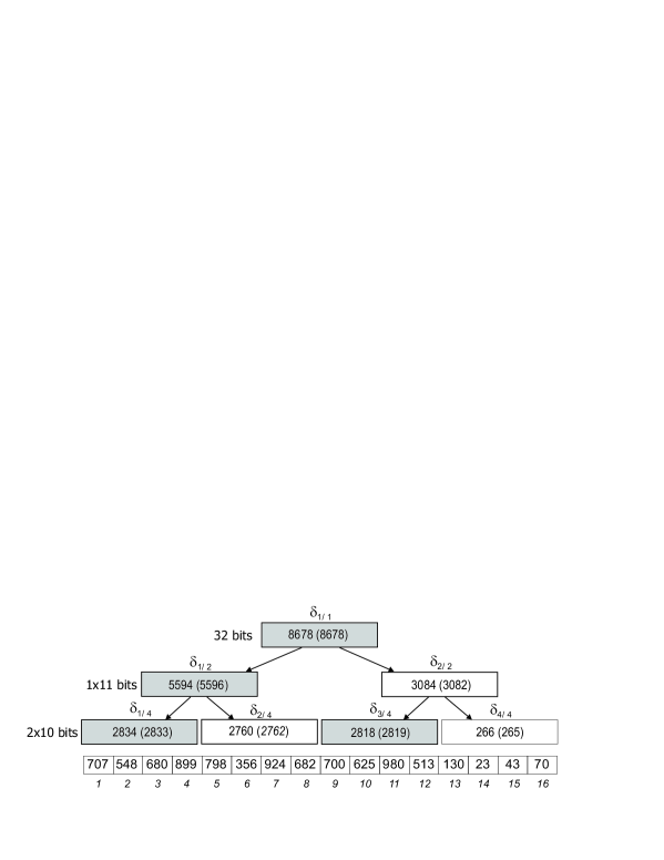
Figure 1: The 3-level tree.

We are now ready to solve the frequency estimation inside the bucket $B$. Given $d$, $1\leq d<b$, let $i$ be the integer for which $\lceil(i-1)/4\cdot b\rceil\leq d<\lceil i/4\cdot b\rceil$. Then the approximate value of $F[d]$ is:

$$\begin{array}[]{l}\widetilde{F}[d]=P(i)+P^{\prime}(i)+\frac{d-\lceil(i-1)/4\cdot b\rceil}{\lceil i/4\cdot b\rceil-\lceil(i-1)/4\cdot b\rceil}\cdot\widetilde{\delta}_{i/4}\end{array}$$

where

$$\begin{array}[]{ll}P(i)=\left\{\begin{array}[]{ll}\widetilde{\delta}_{1/2}&\mbox{if $i>2$}\\ 0&\mbox{if $i\leq 2$}\end{array}\right.&\ \ \ \ \ P^{\prime}(i)=\left\{\begin{array}[]{ll}\widetilde{\delta}_{1/4}&\mbox{if $i=2$}\\ \widetilde{\delta}_{3/4}&\mbox{if $i=4$}\\ 0&\mbox{otherwise}\end{array}\right.\\ \end{array}$$

Thus we use the interpolation based on the CVA only inside a segment of length $\lceil(1/4)\cdot b\rceil$. This component becomes zero at each distance $d=\lceil i\cdot\frac{b}{4}\rceil$, $1\leq i<4$.

32 bits may be distributed in such a way that the granularity of the tree-index increases w.r.t. 3LT. 4LT index has 4 levels and uses 6 bits for the first level, 5 bits for the second one and 4 bits for the last level.

4 Level Tree index (4LT) We reserve 4 bits to store the approximate value of each of the following 4 partial sums: $\delta_{1/8}$, $\delta_{3/8}$, $\delta_{5/8}$ and $\delta_{7/8}$ — let $L_{i/8}$, $i=1,3,5,7$, denote such 4-bits strings. We then use the remaining 16 bits as follows: the partial sums $\delta_{1/4}$ and $\delta_{3/4}$ are approximated by the 5-bit strings $L_{1/4}$ and $L_{3/4}$, respectively, while the partial sum $\delta_{1/2}$ with a 6-bits string $L_{1/2}$. As a result, the larger the intervals, the higher is the number of bits used. The 8 $L$ strings are constructed as follows:

$$\small\begin{array}[]{ll}L_{1/2}=\langle\frac{\delta_{1/2}}{\delta_{1/1}}\cdot(2^{6}-1)\rangle&\\ L_{i/4}=\langle\frac{\delta_{i/4}}{\delta_{j/2}}\cdot(2^{5}-1)\rangle&(i=1\wedge j=1),(i=3\wedge j=2)\\ L_{i/8}=\langle\frac{\delta_{i/8}}{\delta_{j/4}}\cdot(2^{4}-1)\rangle&(i=1\wedge j=1),(i=3\wedge j=2),\\ &(i=5\wedge j=3),(i=7\wedge j=4)\\ \end{array}$$

where, we recall, $\langle x\rangle$ stands for $round(x)$.

The approximate values for the partial sums are eventually computed as:

$$\begin{array}[]{ll}\widetilde{\delta}_{1/1}=\delta_{1/1}=c&\\ \widetilde{\delta}_{1/2}=\frac{L_{1/2}}{2^{6}-1}\times\widetilde{\delta}_{1/1}\\ \widetilde{\delta}_{2/2}=\widetilde{\delta}_{1/1}-\widetilde{\delta}_{1/2}&\\ \widetilde{\delta}_{i/4}=\frac{L_{i/4}}{2^{5}-1}\times\widetilde{\delta}_{j/2}&(i=1\wedge j=1),(i=3\wedge j=2)\\ \widetilde{\delta}_{i/4}=\widetilde{\delta}_{j/2}-\widetilde{\delta}_{i-1/4}&(i=2\wedge j=1),(i=4\wedge j=2)\\ \widetilde{\delta}_{i/8}=\frac{L_{i/8}}{2^{4}-1}\times\widetilde{\delta}_{j/4}&(i=1\wedge j=1),(i=3\wedge j=2)\\ &(i=5\wedge j=3),(i=7\wedge j=4)\\ \widetilde{\delta}_{i/8}=\widetilde{\delta}_{j/4}-\widetilde{\delta}_{i-1/8}&(i=2\wedge j=1),(i=4\wedge j=2)\\ &(i=6\wedge j=3),(i=8\wedge j=4)\end{array}$$

Similarly to the 3LT-index, the 4LT-index refers to a 4-level tree whose nodes store directly or indirectly the approximate values of the cumulative frequencies for fixed hierarchical intervals starting from the root which stores the overall cumulative frequency $c$.

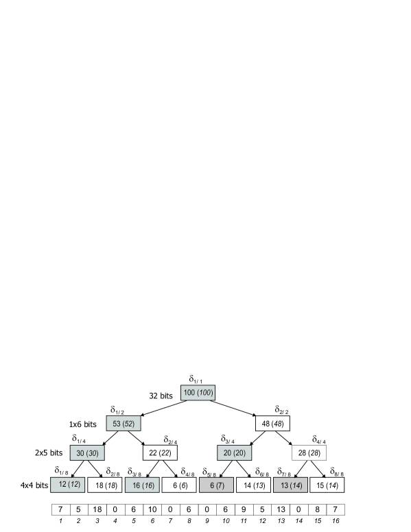
Figure 2: The 4-level tree.

Example 2

Consider the 4-level tree in Figure 2. The 32 bits store the following approximate cumulative frequencies: $L_{1/2}=33$, $L_{1/4}=18$, $L_{3/4}=13$, $L_{1/8}=6$, $L_{3/8}=11$, $L_{5/8}=5$, $L_{7/8}=7$.

Again, similarly to the 3LT-index, the frequency estimation inside the bucket $B$ can be obtained by exploiting the content of the nodes of the index. Given $d$, $1\leq d<b$, and the integer $i$ which $\lceil(i-1)/8\times b\rceil\leq d<\lceil i/8\times b\rceil$, the approximate value of $F[d]$ is:

$$\begin{array}[]{l}\widetilde{F}[d]=P(i)+P^{\prime}(i)+P^{\prime\prime}(i)+\frac{d-\lceil(i-1)/8\times b\rceil}{\lceil i/8\times b\rceil-\lceil(i-1)/8\times b\rceil}\times\widetilde{\delta}_{i/8}\end{array}$$

where

$$\begin{array}[]{ll}P(i)=\left\{\begin{array}[]{ll}\widetilde{\delta}_{1/2}&\mbox{if $i>4$}\\ 0&\mbox{if $i\leq 4$}\end{array}\right.&P^{\prime}(i)=\left\{\begin{array}[]{ll}\widetilde{\delta}_{1/4}&\mbox{if $i=3,4$}\\ \widetilde{\delta}_{3/4}&\mbox{if $i=7,8$}\\ 0&\mbox{otherwise}\end{array}\right.\\ \end{array}$$

$$P^{\prime\prime}(i)=\left\{\begin{array}[]{ll}\widetilde{\delta}_{i-1/8}&\mbox{if $i$ is even}\\ 0&\mbox{otherwise}\end{array}\right.$$

Thus we use the interpolation like in CVA only inside a segment of length $\lceil(1/8)b\rceil$. This component becomes zero at each distance $d=\lceil i\times b/8\rceil$, $1\leq i<8$. We call the estimation 4-level tree or 4LT for short.

3.4 Worst-case Error Analysis

The approximation error for CVA, 1b, USA and 2s arises only from interpolation. On the contrary, for other methods (i.e., 4s, 8s, 3LT and 4LT), the scaling error due to bit saving is added to the interpolation error. However, all methods but CVA, 1b and USA implement a equi-size division of the bucket and 3LT and 4LT provide also an index over sub-buckets. We expect that such a division into sub-buckets produces an improvement from the side of the interpolation error. Indeed, sub-buckets increase the granularity of summarization. In addition, we expect that index-based methods (i.e., 3LT and 4LT), reduce the scaling error, since hierarchical tree-like organization allows us to represent the sum inside a given sub-bucket, corresponding to a node of the tree, as a fraction of the sum contained in the parent node, instead of a fraction of the entire bucket sum (as it happens for the ”flat” methods 4s and 8s). The worst-case analysis confirms the above observations. In particular we show that while CVA, 1b and USA are the same, under the worst-case point of view, 4LT outperforms the other methods.

Results of our analysis are summarized in the following theorem. Recall that, throughout the whole section, a bucket $B$ of size $b$ is given.

Theorem 3.1

Let $F$ be the maximum frequency value occurring in $B$ and let assume that $b$ mod $8=0$. Then, the interpolation and scaling worst-case errors of CVA, 1b, USA, 2s, 4s, 8s, 3LT and 4LT are the following:

error/method	CVA	1b	USA	2s	4s	8s	3LT	4LT
interpolation	$\frac{F\cdot b}{4}$	$\frac{F\cdot b}{4}$	$\frac{F\cdot b}{4}$	$\frac{F\cdot b}{8}$	$\frac{F\cdot b}{16}$	$\frac{F\cdot b}{32}$	$\frac{F\cdot b}{16}$	$\frac{F\cdot b}{32}$
scaling	0	0	0	0	$\frac{F\cdot b}{2^{9}}$	$\frac{F\cdot b}{32}$	$\frac{F\cdot b}{2^{12}}$	$\frac{F\cdot b}{2^{7}}$
total	$\frac{F\cdot b}{4}$	$\frac{F\cdot b}{4}$	$\frac{F\cdot b}{4}$	$\frac{F\cdot b}{8}$	$\frac{F\cdot b}{16}$	$\frac{F\cdot b}{16}$	$\frac{F\cdot b}{16}$	$\frac{F\cdot b}{32}$

Proof

Let $b_{M}$ the size of the smallest sub-bucket produced by the method $M$, where $M$ is either CVA, 1b, USA, 2s, 4s, 8s, 3LT or 4LT. Observe that $b_{M}=b$ for CVA, 1b and USA (since they do not produce sub-buckets), while $b_{2s}=\frac{b}{2}$, $b_{M}=\frac{b}{4}$ for $M=$ 4s or $M=$ 3LT, $b_{M}=\frac{b}{8}$ otherwise.

Consider first the interpolation error (by assuming that no scaling error occurs).

Interpolation error bounds. It can be easily verified that the worst case for a method $M$ happens whenever both the following conditions hold:

1. there is a smallest sub-bucket, say $B$ (of size $b_{M}$) containing, in the first half, $\frac{b_{M}}{2}$ frequencies with value $F$, and, in the second half, $\frac{b_{M}}{2}$ frequencies with value 0, and

2. the range query involves exactly the first half of the sub-bucket $B$.

The proof of this part is conducted separately for each method, by determining the maximum absolute interpolation error:

CVA: In this case, $b_{M}=b$, that is the sub-bucket coincides with the entire bucket and the query boundaries are $1$ and $\frac{b}{2}$. The cumulative value of the bucket is $F\cdot\frac{b}{2}$. Under CVA, the estimated value of the query is $\frac{F\cdot\frac{b}{2}}{b}\cdot\frac{b}{2}$, that is $\frac{F\cdot b}{4}$. The actual value of the query is $\frac{F\cdot b}{2}$. Therefore the absolute error is $\frac{F\cdot b}{4}$.

1b: We obtain the same absolute error $\frac{F\cdot b}{4}$. Indeed, being the first value of the bucket $F$ (i.e., not null), 1-biased estimation does not give additional information w.r.t. CVA.

USA: Also in this case, $b_{M}=b$, that is the sub-bucket coincides with the entire bucket and the query boundaries are $1$ and $\frac{b}{2}$. The cumulative value of the bucket is $F\cdot\frac{b}{2}$. USA assumes that the $\frac{b}{2}$ non null values are located at equal distance from each other, and each has the value $F$. As a consequence the estimated value of the query is $F\cdot\frac{b}{4}$, since the query involves just half non null estimated values. The actual value is $\frac{F\cdot b}{2}$. Thus, the absolute error is $\frac{F\cdot b}{4}$, that is the same as CVA.

2s: In this case $b_{M}=\frac{b}{2}$. According to the case CVA, the absolute error is $\frac{F\cdot b_{M}}{4}$, that is $\frac{F\cdot b}{8}$.

4s and 3LT: Both 4s and 3LT produce sub-buckets of size $\frac{b}{4}$. Thus, in these cases $b_{M}=\frac{b}{4}$. Identically to the previous case, the absolute error is $\frac{F\cdot b_{M}}{4}$, that is $\frac{F\cdot b}{16}$.

8s and 4LT: Both 8s and 4LT produce sub-buckets of size $\frac{b}{8}$. Thus, in these cases $b_{M}=\frac{b}{8}$. Identically to the previous case, the absolute error is $\frac{F\cdot b_{M}}{4}$, that is $\frac{F\cdot b}{32}$.

Now we consider the scaling error.

Scaling error bounds. The proof that CVA, 1b, USA and 2s do not produce scaling error is straightforward. Let us consider the other methods:

4s: Since each sub-bucket sum is encoded by 8 bits and is scaled w.r.t. the overall bucket sum, the maximum scaling error is $\frac{F\cdot b}{2^{9}}$.

8s: Since each sub-bucket sum is encoded by 4 bits and scaled w.r.t. the overall bucket sum, the maximum scaling error is $\frac{F\cdot b}{2^{5}}=\frac{F\cdot b}{32}$.

3LT: In this case, the scaling error may be propagated going down along the path from the root to the leaves of the tree. We may determine an upper bound of the worst-case error by considering the sum of the maximum scaling error at each level. Thus, we obtain the following upper bound: $\frac{\frac{F\cdot b}{2^{12}}+\frac{F\cdot b}{2}}{2^{11}}$. Indeed, the maximum scaling error of the first level is $\frac{F\cdot b}{2^{12}}$. The above value is obtained by considering that the maximum sum in the half bucket corresponding to the first level is $\frac{F\cdot b}{2}$, and that going down to the second level introduces a maximum scaling error obtained by dividing the overall sum by $2^{11}$. Thus, the maximum scaling error for 3LT is $\Theta(\frac{F\cdot b}{2^{12}})$ (that is, the scaling error of the first level).

4LT: For 4LT can be applied the same argumentation as 3LT, by obtaining that the maximum scaling error is of the same order as the first level. That is, $\Theta(\frac{F\cdot b}{2^{7}})$, since the first level uses 6 bits.

The proof is thus completed.

It is worth noting that, as expected, 4LT and 8s produce the smallest interpolation worst-case error, that is $\frac{F\cdot b}{32}$. Considering also the results about scaling error, the overall conclusion we may draw from the above analysis is that the best two methods w.r.t. interpolation, that is 8s and 4LT, are not the same in terms of scaling error. Indeed 4LT shows a relevant accuracy improvement since the error goes from $\frac{F\cdot b}{2^{5}}$ of 8s to $\frac{F\cdot b}{2^{7}}$ of 4LT.

In the next subsection we shall perform a number of experiments to provide additional arguments in favor of the superiority of 4LT estimation, by performing also an average-case analysis of methods under a number of meaningful data distributions. We shall not conduct experiments on the CVA because we are aware that CVA uses 32 bits less and, therefore, could reduce the size of the bucket, thus providing a better accuracy. Actually, the performance analysis coincides with the one of 2s estimation, that is CVA in half bucket.

3.5 Experiments inside a Bucket

In this section we report the results of a large number of experiments performed with various synthetic data sets obtained with different distributions. We measure the accuracy of all the above mentioned methods in estimating range queries inside a bucket. In particular, the methods considered are: USA, 1b, 2s, 8s, 3LT and 4LT. We observe that the space required for storing a bucket is the same for all the considered methods. Experiments are conducted on synthetic data generated according several data distributions. A data distribution is characterized by a distribution for frequencies and a distribution for spreads. Frequency set and value set are generated independently, then frequencies are randomly assigned to the elements of the value set.

3.5.1 Test Bed.

In this section we illustrate the test bed used in our experiments. In particular, we describe (1) the data distributions, that is the probability distributions used for generating frequencies in the tested buckets, (2) the bucket populations, that is the set of parameters characterizing bucket used for generating them under the probability distributions, (3) the data sets, that is the set of samples produced by the combination of (1) and (2), (4) the query set and error metrics, that is the set of query submitted to sample data and the metrics used for measuring the approximation error.

Data Distributions: We consider four data distributions: (1) Zipf-$cusp\_max$ (0.5,1.0): Frequencies are distributed according to a Zipf distribution Zipf49Human with the $z$ parameter equal to $0.5$. Spreads are distributed according to a Zipf $cusp\_max$ Poo97 (i.e., increasing spreads following a Zipf for the first half elements and decreasing spreads following a Zipf distribution for the remaining elements) with $z$ parameter equal to $1.0$. (2) Zipf-$cusp\_max$(1.0,1.0). (3) Zipf-$cusp\_max$(1.5,1.0). (4) Gauss-rand: Frequencies are distributed according to a Gauss distribution with standard deviation $1.0$. Spreads are randomly distributed as well.

Bucket Populations: A population is characterized by the values of $c$ (overall cumulative frequency), $b$ (the bucket size) and $t$ (number of non-null attribute values) and consists of all buckets having such values. We consider 9 different populations divided into two sets, that are called t-var and b-var, respectively.

Set of populations t-var. It is a set of 6 populations of buckets, all of them with $c=20000$ and $b=500$. The 6 populations differ on the value of the parameter $t$ ($t$=10, 100, 200, 300, 400, 500), and are denoted by t-var(10), t-var(100), t-var(200), t-var(300), t-var(400) and t-var(400), respectively.

Set of populations b-var. It is a set of 4 populations of buckets, all of them with $c=20000$. They differ on the value of the parameters $b$ and $t$. We consider $4$ different values for $b$ ($b$=100, 200, 500, 1000). The number of non-null values $t$ of each population is fixed in a way that the ratio $t/b$ is constant and equal to $0.2$; so the values of $t$ are 20, 40, 100 and 200. The four populations are denoted by b-var(100), b-var(200), b-var(500) and b-var(1000).

Moreover, a generic population whose parameter values are, say, $\bar{c}$, $\bar{b}$ and $\bar{t}$ (for $c$, $b$ and $t$, respectively), is denoted by p($\bar{c}$, $\bar{b}$, $\bar{t}$).

Data Sets: As a data set we mean a sampling of the set of buckets belonging to a given population following a given data distribution. Each data set included in the experiments is obtained by generating $100$ buckets belonging to one of the populations specified above under one of the above described data distributions. We denote a data set by the name of the data distribution and the name of the population. For example, the data set (Zipf-cusp_max(0.5,1.0), b-var(200)) denotes a sampling of the set of buckets belonging to the population of b-var corresponding to the value 200 for the parameter $b$ following the data distribution Zipf-cusp_max(0.5,1.0).

We generate 23 different data sets classified as follows: (1) Zipf-t (i.e., Zipf data, different bucket density), containing the five data sets (Zipf-cusp_max(0.5,1), t-var($t$)), for $t$=10, 100, 200, 300, 400, 500. (2) Zipf-b (i.e., Zipf data, different bucket size), containing the four data sets (Zipf-cusp_max(0.5,1), b-var($b$)), for $b$=100, 200, 500, 1000. (3) Gauss-t (i.e., Gauss data, different bucket density), containing the five data sets (Gauss-rand, t-var($t$)), for $t$=10, 100, 200, 300, 400, 500. (4) Gauss-b (i.e., Gauss data, different bucket size), containing the four data sets (Gauss-rand, b-var($b$)), for $b$=100, 200, 500, 1000. (5) Zipf-z (i.e., Zipf data, different skew), containing the three data sets Zipf-cusp_max($z$,1.0), p(20000,400,200)), for $z$=0.5, 1.0, 1.5. Recall that p(20000,400,200) denotes the population characterized by $c=20000,b=400,t=200$.

Each class of data sets is designed for studying the dependence of the accuracy of the various methods on a different parameter (parameter $t$ measuring the density of the bucket, parameter $b$ measuring the size of the bucket and parameter $z$, measuring the data skew). For each data set, 1000 different samples obtained by permutation of frequencies was generated and tested, in order to give statistical significance to experiments.

Query set and error metrics: We perform all the queries $S[d]$, for all $1\leq d<b$. We measure the error of approximation made by the various estimation techniques on the above query set by using both:

• the average of the relative error $\frac{1}{b-1}\sum_{d=1}^{b-1}e_{d}^{rel}$, where $e_{d}^{rel}$ is the relative error of the query with range $d$, i.e., $e_{d}^{rel}=\frac{|{S[d]-\widetilde{S}[d]}|}{S[d]}$, and

• the normalized absolute error, that is the ratio between the average absolute error and the overall sum of the frequencies in the bucket, i.e. $\sum_{d=1}^{b-1}\frac{|{S[d]-\widetilde{S}[d]}|}{c\cdot b}$

where $\widetilde{S}[d]$ is the value of $S[d]$ estimated by the technique at hand.

3.5.2 Results of Experiments and Discussion.

In this section we give a qualitative discussion about the approximation error of the considered methods, excluding USA and 1-biased, about which we have already provided a theoretical analysis in Section 3.4. First we consider methods working simply by splitting the original bucket, that are 2s, 4s and 8s. For all these methods, the estimation error may arise from the following approximation sources:

1. the linear interpolation (i.e., CVA), concerning the evaluation of the query inside the “smallest” sub-buckets (for instance, in the case of the 4s, the smallest sub-buckets are the quarts of the bucket),

2. the numeric approximation, in case sums are stored by less than 32 bits (note that only 2s is not affected by this error).

We call error of type 1 and 2, respectively, the above described components of the approximation error.

Relative error vs data density.

Concerning error of type 1, what we expect is that, for all methods, it increases as data sparsity increases. Indeed, in case of sparse data, the sum tends to concentrate in a few points, and this reduces the suitability of linear interpolation to approximate the frequency distribution. Moreover, we expect that such a component of the error decreases as splitting degree increases: for instance, in case of 8s, which splits the bucket into 8 parts, we expect more accuracy (in terms of the error of type 1) than the 2s method. The reason is that having smaller sub-buckets means applying linear interpolation to shorter (and, thus, better linearly-approximable) segments of the cumulative frequency distribution.

About error of type 2 we expect that both (i) it increases as the splitting degree increases and (ii) it is independent of data sparsity. Claim (i) is explained by considering that increasing the splitting degree means reducing the number of bits used for representing the sum of sub-buckets. Claim (ii) is related to the numeric nature of the error.

The observations above show the existence of a trade-off between the need of increasing the splitting degree for improving CVA precision on one hand, and the need of using as more bits as possible for representing partial sums in the bucket on the other hand. However, we expect that such a trade-off is more evident in case of high splitting degree, that is, when the error of type 2 is more relevant. For instance, recalling that the maximum absolute error of type 2 is $\frac{c}{2^{k+1}}$, where $k$ is the number of bits assigned to smallest sub-buckets, being $k=4$ for 8s and $k=8$ for 4s, the maximum absolute error of type 2 for 8s in case $c=20000$ is 625 (i.e., about the 3% of $c$) while it is 39 (i.e., a negligible percentage of $c$) for 4s.

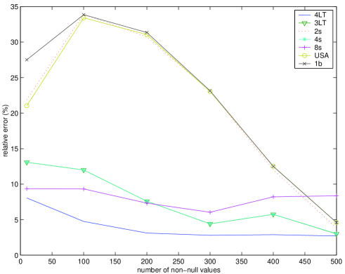
(a): Error for different values of $t$

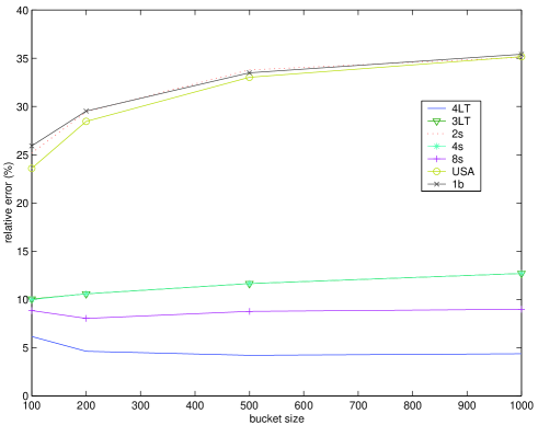
(b): Error for different values of $b$

Figure 3: Experimental Results for data sets Zipf

Experiments confirm the above considerations. By looking at graphs of Figure 3.(a) we may observe that for 2s and 4s the error decreases as the data density increases. On the contrary, for 8s, the error is quasi-constant (slightly increasing) in case of Zipf distributions, while it is slightly decreasing (but much less quickly than 4s) in case of Gauss distribution (see Figure 4.(a)). Concerning the comparison between 2s, 4s and 8s, we may observe in Figures 3.(a) that for low values of data density, as expected, accuracy of 8s is higher than 4s and, in turn, accuracy of 4s is higher than 2s. But, as observed above, for increasing data density, trends of 4s and 8s suffer, in a different measure, the presence of the error of type 2. This appears quite evident in Figure 3.(a), whereby we may note that 8s becomes worse than 4s from about 210 non null elements on and the improving trend of 2s is considerable faster than the other methods (since 2s does not suffer the error of type 2).

We observe that USA gives better estimation than $1b$ on Zipf data (see Figures 3.(a)). Accuracy of USA becomes the worst when the data sets follow the Gauss distribution (see Figures 4.(a)). This proves that the assumption made by USA can be applicable for particular distributions of frequencies and spreads, like those of data sets Zipf-t. Results obtained on data sets distributed according a Gauss distribution confirm the above claim: accuracy of USA becomes the worst when the data sets have a random distribution as it happens for Gauss-t (see Figure 4.(a)).

Concerning 1b we may observe that the behaviours of $1b$ and 2s are similar. As expected, the exploitation of the information that the bucket is 1-biased does not give a significant contribution to the accuracy of the estimation. Indeed, the knowledge of the position of just one element in the bucket does not add in general appreciable information.

Consider now the usage of the tree-indices 3LT and 4LT. Recall that 3LT has the same splitting degree of 4s, since both methods divide the bucket into 4 sub-buckets. Possible difference in terms of accuracy between the two methods may arise from error of type 2. Indeed, the tree-like organization of indices allows us to represent the sum inside a given sub-bucket corresponding to a node of the tree as a fraction of the sum contained in the parent node, instead of the entire sum (as it happens for the ”flat” methods). Thus, we expect that tree-indices produce smaller errors of type 2. However, as previous noted, 4s produces a negligible percentage of error of type 2. This explains why 3LT and 4s basically present the same error (lines in the graphs are almost entirely overlapped).

4LT has the same splitting degree as 8s (since both methods divide the bucket into 8 sub-buckets). As a consequence, being appreciable the error of type 2 of the 8s (as already discussed), we may expect improvements by the usage of 4LT. This is that results from experiments. 4LT has the best performances: it shows only benefits deriving from the increasing of data density (producing the reduction of error of type 1), with no appreciable increasing of error of type 2. 4LT, thanks to the tree-like organization of the sums, seems to solve the trade-off between increasing splitting degree (for improving CVA precision) and controlling numeric error arising from the usage of a reduced number of bits for representing sums.

Relative error vs bucket size and data skew.

First consider populations b-var. Recall that for such data sets we have maintained constant the data density around 20%. Thus, increasing the bucket size means increasing also non-null elements. While, as for previous experiments, error of type 2 is independent of the bucket size, (even though all the above considerations about the relationship between error of type 2, splitting degree and number of bits per smallest sub-buckets are still valid), we expect that CVA precision suffers the variation of the bucket size. Indeed, on the one hand the CVA precision decreases as the bucket size increases, since, for a larger bucket, linear interpolation is applied to a larger segment of the cumulative frequency. But, on the other hand, increasing the bucket size means increasing the number of non-null elements (keeping constant the overall sum) and this means reducing the probability that the sum is concentrated into a few picks. Thus, whenever the cumulative frequency is smooth, linear interpolation tends to give better results. Depending on data distribution, we may observe either that the two opposite component compensate each other or one prevails over the other. Indeed, experiments with Zipf data, corresponding to Figure 3.(b), show that methods have a quasi-constant trend (with a slight prevalence of the first component), while experiments conducted on Gauss data, corresponding to Figure 4.(b), show a net prevalence of the second component (all the methods present a decreasing trend for increasing bucket size). Such experiments do not give new information about the comparison between the considered methods, confirming substantially the previous results. Again 4LT has the best performance.

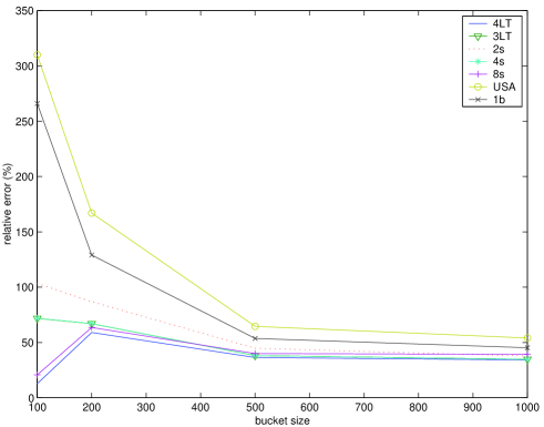
(a): Data sets Gauss-t: error for different values of $t$

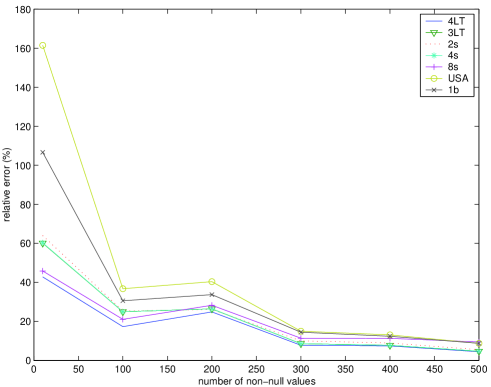
(b): Data sets Gauss-D: error for different values of $b$

Figure 4: Experimental Results for data sets Gauss

Results of experiments conducted on the class of data sets Zipf-z, for measuring the dependence of the accuracy of methods on the data skew are reported in Figure 5. We note that all methods become worse as $z$ increases (as it can be intuitively expected). The behaviours of $1b$ and 2s are similar, while 4LT shows the best performance.

As a final remark we may summarize the comparison between the considered methods concluding that the worst method is always 2s, followed by 8s and then by 3LT and 4s for sparse data. On the contrary, for dense data 3LT and 4s show better performance than 8s. Observe that 4s and 3LT have basically the same accuracy. The best methods appears definitely 4LT.

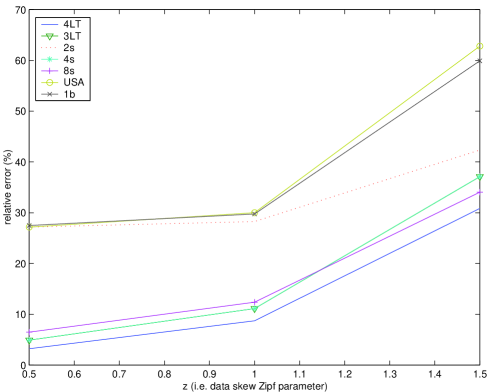
Figure 5: Data sets Zipf-z: dependence on data skew

4 Applying the 4LT Index to the Entire Histogram

The analysis described in the previous sections suggests to apply the technique of the 4-level tree index to a whole histogram in order to improve its accuracy on the approximation of the underlying frequency set. We stress that the problem of investigating whether such an addition is really convenient is not straightforward: observe that 4LT buckets use 32 bits more than CVA ones, and, then, for a fixed storage space, allow a smaller number of buckets. In this section we show how to combine the 4LT technique with classical methods for constructing histograms and we perform a large number of experiments to measure the effective improvement given by the usage of the 4LT. The advantage of the 4LT index is shown to be relevant also when it is compared with buckets using CVA, that is, when the storage space required by 4LT is larger than the original method. Moreover, the 4LT index shows very good performances if it is combines with a very simple method for constructing histograms, called EquiSplit, consisting on partitioning the attribute domain into equal-size buckets. Let us start with a quick overview of the most relevant methods proposed so far for the construction of histograms.

4.1 Methods for Constructing Histograms

Besides the method used for approximating frequencies inside buckets, the capability of a histogram of accurately approximating the underlying frequency set strongly depends on the way such a set is partitioned into buckets. Typically, criteria driving the construction of a histogram is the minimization of the error of the reconstruction of the original (cumulative) frequency set from the histogram. Partition rules proposed in Poosala96Improved ; Jagadish98Optimal , try to achieve this goal. Among those, we sketch the description of two well-known approaches: MaxDiff and V-optimal (see Poosala96Improved ; Poo97 for an exhaustive taxonomy). Note that these methods are defined for 2-histograms but are in practice mainly used for 1-histograms to minimize storage consumption.

MaxDiff. A MaxDiff histogram Cri81 ; Poosala96Improved of size $h$ is obtained by putting a boundary between two adjacent attribute values $v_{i}$ and $v_{i+1}$ of $V$ if the difference between $f(v_{i+1})\cdot\sigma_{i+1}$ and $f(v_{i})\cdot\sigma_{i}$ is one of the $h-1$ largest such differences (where $\sigma_{i}$ denotes the spread of $v_{i}$). The product $f(v_{i})\cdot\sigma_{i}$ is said the area of $v_{i}$.

V-Optimal. A V-Optimal histogram Poosala96Improved ; Jagadish98Optimal gives very good performances. It is obtained by selecting the boundaries for each bucket, $inf_{i}$ and $sup_{i}$, $1\leq i\leq n$, so that $\sum_{i=1}^{n}SSE_{i}$ is minimal, where $SSE_{i}=\sum_{j=inf_{i}}^{sup_{i}}(f(j)-avg_{i})^{2}$ and $avg_{i}$ is equal to the average frequency in the $i$-th bucket, thus the cumulative frequency in the whole bucket divided by the size $sup_{i}-inf_{i}+1$.

We now propose to combine both methods, MaxDiff and V-Optimal,with the 4LT index in order to have an approximate representation of frequency distributions inside the buckets. We shall compare the so-revised methods with the original ones with CVA estimation at parity of storage consumption. The results will show that the 4LT index very much increases the estimation accuracy of both methods. The additional estimation power carried by the 4LT index even enables a very simple method like the one described below to produce very accurate estimations.

EquiSplit. The attribute domain is split into $k$ buckets of approximately the same size $b=\lceil m/k\rceil$. In this way, as the boundaries of all buckets can be easily determined from the value $b$, we only need to store a value for each bucket: the sum of all frequencies. This method has been first introduced in Cri81 and, as the experimental analysis will confirm, it has very good performances for low skewed data, while its performances get worse in case of high skew.

4.2 Experiments on Histograms

In this section we shall conduct several experiments both on synthetic and real-life data in order to compare the effectiveness of several histograms in estimating range query size.

Experiments on Synthetic Data.

First we present the experiments performed on synthetic data. Below we describe data sets, error metrics and the query set considered in our experiments.

Available Storage: Note that under CVA each bucket stores only two integers, while with the 4LT index each bucket needs three integers. Assuming 32 bits the storage space for an integer, given a fixed $K$ number of bits for the total storage space required for the whole histogram, both MaxDiff and V-Optimal under CVA produce $\lfloor\frac{K}{64}\rfloor$ buckets while both of them with 4LT indices only produce $\lfloor\frac{K}{96}\rfloor$ buckets. On the other hand, a bucket for EquiSplit just needs one integer (the sum of all the frequencies), while for EquiSplit-4LT it needs two integers. Thus, for a fixed $K$ number of bits for the total storage space, EquiSplit with CVA produces $\lfloor\frac{K}{32}\rfloor$ and EquiSplit with 4LT indices produces $\lfloor\frac{K}{64}\rfloor$ as $MD\_CVA$.

For our experiments, we shall use a storage space, that is $42$ four-byte numbers to be in line with experiments reported in Poosala96Improved ; Jagadish98Optimal , which we replicate. Using the above considerations, it can be easily realized that MaxDiff with CVA, V-Optimal with CVA, and EquiSplit with 4LT indices produce 21 buckets, EquiSplit with CVA produces 42 buckets, and both MaxDiff and V-Optimal with 4LT indices only produce 14 buckets.

Data Distributions: A data distribution is characterized by a distribution for frequencies and a distribution for spreads. Frequency set and value set are generated independently, then frequencies are randomly assigned to the elements of the value set. We consider 5 data distributions: (1) $D_{1}$: Zipf-$cusp\_max$(0.5,1.0). (2) $D_{2}=$ Zipf-zrand(0.5,1.0): Frequencies are distributed according to a Zipf distribution with the $z$ parameter equal to $0.5$. Spreads follow a $ZRand$ distribution Poo97 with $z$ parameter equal to $1.0$ (i.e., spreads following a Zipf distributions with $z$ parameter equal to $1.0$ are randomly assigned to attribute values). (3) $D_{3}=$ Gauss-rand: Frequencies are distributed according to a Gauss distribution with standard deviation $1.0$. Spreads are randomly distributed. (4) $D_{4}=$ Zipf-$cusp\_max$(1.5,1.0). (5) $D_{5}=$ Zipf-$cusp\_max$(3.0,1.0).

Histograms Populations: A population is characterized by the value of three parameters, that are $T$, $D$ and $t$ and represents the set of histograms storing a relation of cardinality $T$, attribute domain size $D$ and value set size $t$ (i.e., number of non-null attribute values).

Population $P_{1}$. This population is characterized by the following values for the parameters: $D=4100$, $t=500$ and $T=100000$.

Population $P_{2}$. This population is characterized by the following values for the parameters: $D=4100$, $t=500$ and $T=500000$.

Population $P_{3}$. This population is characterized by the following values for the parameters: $D=4100$, $t=1000$ and $T=500000$.

Data Sets: Similarly to the experiments inside buckets, each data set included in the experiments is obtained by generating under one of the above described data distributions $10$ histograms belonging to one of the populations specified below. We consider the 15 data sets that are generated by combining all data distributions and all populations.
All queries belonging to the query set below are evaluated over the histograms of each data set:

Query set and error metrics: In our experiments, we use the query set $\{X\leq d:d\in{{\cal U}}\}$ (recall that $X$ is the histogram attribute and ${{\cal U}}$ is its domain) for evaluating the effectiveness of the various methods. We measure the error of approximation made by histograms on the above query set by using the average of the relative error $\frac{1}{Q}\sum_{i=1}^{Q}e_{i}^{rel}$, where $Q$ is the cardinality of the query set and $e_{i}^{rel}$ is the relative error , i.e., $e_{i}^{rel}=\frac{|{S_{i}-\widetilde{S}_{i}}|}{S_{i}}$, where $S_{i}$ and $\widetilde{S}_{i}$ are the actual answer and the estimated answer of the query $i$-th of the query set.

4.2.1 Results of the Experiments.

In Tables 1, 2 and 3 the results of experiments conducted on all data sets are reported. We denote the methods MaxDiff, V-Optimal and EquiSplit with CVA by MD, VO and ES, respectively; these methods with 4LT indices are denoted by MD_4LT, VO_4LT, ES_4LT.

$method/distr.$	$D_{1}$	$D_{2}$	$D_{3}$	$D_{4}$	$D_{5}$
$ES$	$0.79$	$1.69$	$10.61$	$3.89$	$57.63$
$ES\_4LT$	$0.29$	$0.84$	$2.01$	$2.89$	$29.63$
$MD$	$4.29$	$19.37$	$11.65$	$7.02$	$31.46$
$MD\_4LT$	$0.70$	$1.57$	$3.14$	$1.92$	$4.39$
$VO$	$1.43$	$5.55$	$10.6$	$5.16$	$21.57$
$VO\_4LT$	$0.29$	$1.33$	$2.32$	$1.62$	$3.15$

Table 1: Pop. 1: error for various methods.

$method/distr.$	$D_{1}$	$D_{2}$	$D_{3}$	$D_{4}$	$D_{5}$
$ES$	$0.76$	$1.78$	$4.83$	$3.63$	$59.74$
$ES\_4LT$	$0.28$	$0.84$	$6.40$	$1.40$	$31.12$
$MD$	$5.79$	$16.04$	$6.65$	$13.56$	$33.51$
$MD\_4LT$	$0.80$	$1.60$	$2.32$	$2.36$	$4.87$
$VO$	$1.68$	$5.96$	$6.16$	$7.25$	$18.10$
$VO\_4LT$	$0.32$	$1.41$	$4.85$	$1.53$	$3.12$

Table 2: Pop. 2: error for various methods.

$method/distr.$	$D_{1}$	$D_{2}$	$D_{3}$	$D_{4}$	$D_{5}$
$ES$	$0.47$	$0.87$	$2.31$	$7.54$	$66.41$
$ES\_4LT$	$0.27$	$0.35$	$1.14$	$3.59$	$25.01$
$MD$	$8.37$	$2.89$	$3.30$	$3.46$	$25.01$
$MD\_4LT$	$0.70$	$0.59$	$1.33$	$1.79$	$2.02$
$VO$	$1.77$	$2.16$	$2.82$	$3.37$	$7.78$
$VO\_4LT$	$0.32$	$0.56$	$1.24$	$1.68$	$1.82$

Table 3: Pop. 3: error for various methods.

The cross behavior of the various methods is similar for the three populations. Experiments confirm the good performance of the MaxDiff method and, particularly, of V-Optimal but they also pinpoint that 4LT adds to both methods relevant benefits. Indeed MD_4LT and VO_4LT show very low errors. Also EquiSplit and EquiSplit-4LT have good performances. But, as shown in Figure 6.(a), where the dependence of the estimation error on data skew is plotted, these methods quickly get worse for high data skew. Indeed, in such cases, the benefit given by the higher number of buckets is lost because of the high skew inside buckets. In case of high skew, partition rules play a central role, and the naive approach of EquiSplit is not suitable. Interestingly, we observe that the improving of MaxDiff and V-Optimal by the usage of 4LT indices is relevant also for high skew, proving the effectiveness of such indices. In Figure 6.(b) we show the dependence of the accuracy of the methods on the amount of space. There, we consider the data distribution $D_{4}$ and the population $P_{1}$ and generate 10 histograms belonging to $P_{1}$ according to $D_{4}$ for different amounts of space. The aim of this experiment is to study the behaviour of the various methods as the compression factor increases. Clearly, when the available amount of space increases, all methods behave well. The differences are more relevant for values corresponding to high compression. Methods using 4TL are the best. This can be intuitively explained by considering that in case of large buckets the role of the approximation technique inside buckets becomes more important than the rules followed for constructing buckets.

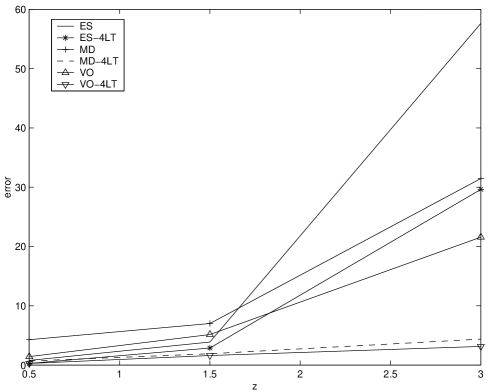
(a): Dependence of the accuracy on the data skew

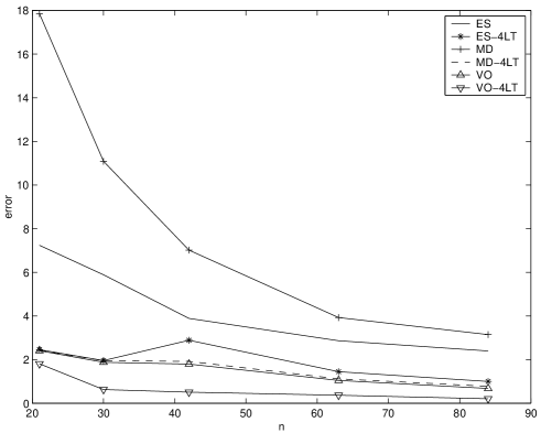
(b): Dependence of the accuracy on the representation

size (i.e., number of stored 4-byte integers)

Figure 6: Experimental Results

Experiments on Real-Life Data.

We have performed further experiments using real-life data. We have considered two data sets (that we denote by Data Set A and Data Set B) obtained from the 1997 U.S. Census Statistics Census , by choosing two attributes of the table Special District Governments, having the following characteristics:

Data Set A: attribute name: Type Code, domain size: $D=998$, number of non-null attribute values: $t=787$, cardinality: $T=34683$.

Data Set B: attribute name: Function Code, domain size: $D=99$, number of non-null attribute values: $t=32$, cardinality: $T=34683$.

We use for each histogram the same amount of storage space, that is $21$ four-byte numbers. Query set and error metrics are the same used for experiments on synthetic data.

method	data set A	data set B
$ES$	4.32	7.02
$ES\_4LT$	0.97	3.59
$MD$	11.30	22.82
$MD\_4LT$	1.63	1.25
$VO$	4.49	17.19
$VO\_4LT$	1.86	3.05

Table 4: Errors obtained on real data.

Results of the Experiments. As shown in Table 4, experiments on real data confirm the results obtained with synthetic data. We note that 4LT adds to MaxDiff and V-Optimal relevant benefits and both EquiSplit and EquiSplit-4LT have good performances. Not surprisingly, for the data set A, EquiSplit-4LT produces the smallest error. This can be explained by considering that data of this set are rather uniform, and, in this case, as discussed previously, the cheapest technique (in terms of storage space) gives the best performances. In other words, the extra storage space required for recording bucket boundaries of the more sophisticate techniques does not give benefits due to the trivial data distribution.

5 Conclusions

In this paper we have presented a technique for improving the frequency estimation within each bucket of a histogram. This technique goes beyond the simple methods used in the literature, that is, the continuous value assumption and the uniform spread assumption. Our method is based on the addition of a 32 data item to each bucket organized into a 4-level tree index (4LT, for short) that stores, in a bit-saving approximate form, a number of hierarchical range queries internal to the bucket. We have shown both theoretically and experimentally that such an additional information effectively allows us to better estimate range queries inside buckets. Interestingly, the usage of 4LT on top of histograms built through well-know techniques like MaxDiff and V-Optimal, outperforms such histograms in terms of accuracy. This claim is proven in the paper through a large number of experiments conducted on both synthetic and real-life data, where classical histograms combined with 4LT are compared with the standard versions (i.e., with no 4LT) under several different data distributions at parity of consumed storage space. It turns out that the price we have to pay in terms of storage space by consuming 32 bits more per bucket w.r.t. CVA-based histograms is overcome by the benefits given by the improvement of precision in estimating queries inside buckets. Thus, the main conclusion we draw is that the 4LT index may represent a general technique that can be combined with any bucket-based histogram for significantly improving its accuracy.

References

- (1) B. Babcock, S. Babu, M. Datar, R. Motwani, and J. Widom. Models and issues in data stream system. In PODS, pages 1–16, 2002.
- (2) F. Buccafurri, F. Furfaro, and D. Saccà. Estimating range queries using aggregate data with integrity constraints: a probabilistic approach. In Proc. of the 8th International Conference on Database Theory, 2001.
- (3) F. Buccafurri, L. Pontieri, D. Rosaci, and D. Saccà. Improving range query estimation on histograms. In Proceedings of the International Conference on Data Engineering, ICDE, pages 628–638, 2002.
- (4) F. Buccafurri, D. Rosaci, and D. Saccà. Compressed datacubes for fast olap applications. In Proceedings of the Int. Conference on Data Warehousing and Knowledge Discovery, DaWaK, pages 65–77, 1999.
- (5) S. Christodoulakis. Estimating selectivities in databases. PhD Thesis, CSRG Report N. 136, Department of Computer Science, University of Toronto, 1981.
- (6) S. Christodoulakis. Implications of certain assumptions in database performance evauation. ACM Trans. Database Syst., 9(2):163–186, 1984.
- (7) Mayur Datar, Aristides Gionis, Piotr Indyk, and Rajeev Motwani. Maintaining stream statistics over sliding windows: (extended abstract). In Proceedings of the thirteenth annual ACM-SIAM symposium on Discrete algorithms, pages 635–644. Society for Industrial and Applied Mathematics, 2002.
- (8) Donko Donjerkovic, Yannis E. Ioannidis, and Raghu Ramakrishnan. Dynamic histograms: Capturing evolving data sets. In ICDE, page 86, 2000.
- (9) S. Guha, N. Koudas, and K. Shim. Data-streams and histograms. In Proceedings of the thirty-third annual ACM symposium on Theory of computing, pages 471–475. ACM Press, 2001.
- (10) Sudipto Guha, Piotr Indyk, S. Muthukrishnan, and Martin Strauss. Histogramming data streams with fast per-item processing. In Proceedings of the 29th International Colloquium on Automata, Languages and Programming, pages 681–692. Springer-Verlag, 2002.
- (11) Yannis Ioannidis. The history of histograms (abridged). In Proceedings of 29th International Conference on Very Large Data Bases. Morgan Kaufmann, 2003.
- (12) Y.E. Ioannidis and V. Poosala. Balancing histogram optimality and practicality for query result size estimation. In Proceedings of the 1995 ACM SIGMOD International Conference on Management of Data, pages 233–244, 1995.
- (13) H. V. Jagadish, Hui Jin, Beng Chin Ooi, and Kian-Lee Tan. Global optimization of histograms. In Proceedings of the 2001 ACM SIGMOD international conference on Management of data, pages 223–234. ACM Press, 2001.
- (14) H. V. Jagadish, N. Koudas, S. Muthukrishnan, V. Poosala, K. C. Sevcik, and T. Suel. Optimal histograms with quality guarantees. In Proc. 24th Int. Conf. Very Large Data Bases, VLDB, pages 275–286, 24–27 1998.
- (15) F. M. Malvestuto. A universal-scheme approach to statistical databases containing homogeneous summary tables. ACM Transactions on Database Systems (TODS), 18(4):678–708, 1993.
- (16) V. Poosala. Histogram-based estimation techniques in database systems. PhD dissertation, University of Wisconsin-Madison, 1997.
- (17) V. Poosala, V. Ganti, and Y.E. Ioannidis. Approximate query answering using histograms. In IEEE Data Engineering Bulletin, volume 22, pages 5–14, 1999.
- (18) V. Poosala, P. J. Haas, Y. E. Ioannidis, and E. J. Shekita. Improved histograms for selectivity estimation of range predicates. In Proceedings of the 1996 ACM SIGMOD international conference on Management of data, pages 294–305. ACM Press, 1996.
- (19) P. Griffiths Selinger, M. M. Astrahan, D. D. Chamberlin, R. A. Lorie, and T. G. Price. Access path selection in a relational database management system. In Proceedings of the 1979 ACM SIGMOD international conference on Management of data, pages 23–34. ACM Press, 1979.
- (20) I. Sitzmann and P. J. Stuckey. Improving temporal joins using histograms. In Database and Expert Systems Applications, pages 488–498, 2000.
-
(21)
1997 U.S. Census Statistics.
http://census.gov/govs/www/gid.html. - (22) Y. Q. Wu, J. M. Patel, and H. V. Jagadish. Using histograms to estimate answer sizes for xml queries. Inform. Syst., 28:33–59, 2003.
- (23) G. K. Zipf. Human behaviour and the principle of least effort. In Addison-Wesley, Reading, Mass., 1949.