Adaptive Cluster Expansion (ACE): A Hierarchical Bayesian Network

Abstract: Using the maximum entropy method, we derive the “adaptive cluster expansion” (ACE), which can be trained to estimate probability density functions in high dimensional spaces. The main advantage of ACE over other Bayesian networks is its ability to capture high order statistics after short training times, which it achieves by making use of a hierarchical vector quantisation of the input data. We derive a scheme for representing the state of an ACE network as a “probability image”, which allows us to identify statistically anomalous regions in an otherwise statistically homogeneous image, for instance. Finally, we present some probability images that we obtained after training ACE on some Brodatz texture images - these demonstrate the ability of ACE to detect subtle textural anomalies.

1 Introduction

The purpose of this paper is to train probabilistic network models of images of homogeneous textures for use in Bayesian decision making. In our past work in this area [1, 2, 3, 4, 5] we successfully used entropic methods to design Markov random field (MRF) models to reproduce the observed statistical properties of textured images. We now wish to formulate a novel MRF structure that requires much less effort to train and use. There are two essential ingredients in our simplification: we do not use hidden variables, and we restrict our attention to hierarchical transformations of the data.

The use of hidden variables is a flexible way of modelling high order correlations in data [6], but it leads to lengthy Monte Carlo simulations to estimate averages over the hidden variables. An MRF without hidden variables is specified by a set of transformation functions, each of which extracts some statistic from the data, and together they provide sufficient information to compute the probability density function (PDF) of the data [4, 5].

We can obtain a wealth of statistical information about the data by restricting our attention to a finite number of well-defined transformation functions. For instance, in [7] a number of useful textural features are presented, which may be used to model and discriminate between various textures that occur in images. However, we wish to design our transformation functions adaptively in a data-driven manner, so that the resulting set is optimised to capture the statistical properties of the data. We choose to use adaptive hierarchical transformation functions, because these not only capture statistical properties at many length scales, but are also very easy to train.

We briefly discussed hierarchical transformation functions in [8], where we conjectured that topographic mappings [9] might be appropriate for connecting together the layers of the hierarchy. We investigated topographic mappings in [10, 11, 12, 13, 14] and found that they could be rapidly trained to produce useful multiscale representations of data. We therefore use multilayer topographic mappings to adaptively design hierarchical transformation functions of data for use in MRF models. In this type of model different layers of the hierarchy measure statistical structure on different length scales, and shorter length scale structures are clustered together and correlated to produce longer length scale structures. We therefore frequently refer to this type of scheme as an adaptive cluster expansion (ACE). By interpreting ACE as a multilayered n-tuple processor we can relate ACE to a multilayered version of WISARD [15].

We demonstrate the ability of ACE to learn the statistical structure of texture by training an adaptive pyramid image processor. There are many ways of displaying the statistical information extracted from the data by such a processor, but we prefer to use what we call a “probability image”, which is generated from the estimated local PDF of the data.

The layout of this paper is as follows. In Section 2 we use the maximum entropy method to estimate the PDF of the data, subject to a set of marginal probability constraints measured using hierarchical transformation functions, to yield an MRF model in closed form (i.e. no undetermined Lagrange multipliers). In Section 3 we extend this result to remove some of the limitations of its hierarchical structure, such a translation non-invariance, and describe the ACE system for producing probability images. In Section 4 we present the result of applying ACE to some textured images taken from the Brodatz set [16].

2 Maximum entropy PDF estimation

In this section we present a derivation of a hierachical maximum entropy estimate $Q_{\textup{mem}}(x)$ of an observed true PDF $P(x)$, where we constrain $Q_{\textup{mem}}(x)$ so that certain marginal PDFs agree with observation. Although we consider only the case of a binary tree, we also present a simple diagrammatic representation of this result that allows us easily to extend it to general trees.

2.1 Basic maximum entropy method

For completeness, we first of all outline the basic principles [17, 18] of the maximum entropy method of assigning estimates of PDFs. Introduce the entropy functional $H$

$$H=-\int dxQ(x)\log(\frac{Q(x)}{Q_{0}(x)})$$ (1)

in which the PDF $Q_{0}(x)$ is used to introduce prior knowledge about $P(x)$. Loosely speaking, $H$ measures the extent to which $Q(x)$ is non-committal about the value that $x$ might take. The maximum entropy method consists of maximising $H$ subject to the following set of constraints

$$\begin{array}[]{rl}C_{1,i}&=\int dxQ(x)y_{i}(x)-\int dxP(x)y_{i}(x)\\ &=0\end{array}$$ (2)

where the $y_{i}(x)$ are the components of a vector $y(x)$ of sampling functions. These constraints ensure that certain average values are the same whether they are measured using $Q(x)$ (i.e. our estimated PDF) or using $P(x)$ (i.e. the observed true PDF). By carefully selecting the $y(x)$ we can optimise the agreement between $Q(x)$ and $P(x)$ as appropriate.

$Q_{\textup{mem}}(x)$ may be found by introducing a vector $\lambda$ of Lagrange multipliers, and functionally differentiating $H-\sum_{i}\lambda_{i}C_{1,i}$ with respect to $Q(x)$ to yield eventually

$$Q_{\textup{mem}}(x)=\frac{Q_{0}(x)\exp(-\lambda.y(x))}{\int dx^{\prime}Q_{0}(x^{\prime})\exp(-\lambda.y(x^{\prime}))}$$ (3)

The undetermined Lagrange vector $\lambda$ must be chosen in such a way that the constraints are satisfied - this is usually a non-trivial problem.

Now we shall consider a special case of the maximum entropy problem in which we carefully design the $y_{i}(x)$ so that they constrain a set of marginal probabilities [5]. Thus we make the following replacements

$$\begin{array}[]{rl}y_{i}(x)&\longrightarrow\delta(y-y(x))\\ \lambda_{i}&\longrightarrow\lambda(y)\end{array}$$ (4)

where $\delta(y-y(x))$ is a Dirac delta function. In the $\{y_{i}(x),\lambda_{i}\}$ version of the maximum entropy problem, by varying the value of an index $i$ we could scan through the set of constraint functions $y_{i}(x)$ and Lagrange multipliers $\lambda_{i}$. However, in the $\{\delta(y-y(x)),\lambda(y)\}$ version of the maximum entropy problem, by varying the value of a variable $y$ we can scan through the set of constraint functions $\delta(y-y(x))$ and Lagrange multipliers $\lambda(y)$.

The modification in Equation 4 causes the constraints in Equation 2 to become

$$\begin{array}[]{rl}C_{2}(y)&\equiv\int dxQ(x)\delta(y-y(x))-\int dxP(x)\delta(y-y(x))\\ &=Q(y)-P(y)\\ &=0\end{array}$$ (5)

where we have defined the PDFs over $y$ as

$$\begin{array}[]{rl}Q(y)&=\int dxQ(x)\delta(y-y(x))\\ P(y)&=\int dxP(x)\delta(y-y(x))\end{array}$$ (6)

Thus the delta function constraints force $Q(y)=P(y)$. Note that we have used a rather loose notation for our PDFs - $P(x)$ and $P(y)$ are in fact different functions of their respective arguments. We have made this choice of notation for simplicity, because the context will always indicate unambiguously which PDF is required.

By analogy with the previous maximum entropy derivation, $Q_{\textup{mem}}(x)$ may be found by functionally differentiating $H-\int dy\lambda(y)C_{2}(y)$ with respect to $Q(x)$ to yield

$$Q_{\textup{mem}}(x) =\frac{Q_{0}(x)\exp(-\lambda(y(x)))}{\int dx^{\prime}Q_{0}(x^{\prime})\exp(-\lambda(y(x^{\prime})))}$$ (7)

$$\longrightarrow Q_{0}(x)f(y(x))$$ (8)

where $\lambda(y(x))$ is an undetermined Lagrange function of $y(x)$. In Equation 8 we present a simpler notation by introducing an undetermined function $f(y(x))$ to absorb the exponential function and the denominator term that appeared in Equation 7. We may impose the constraints in Equation 5, and use the definitions of $Q(y)$ and $P(y)$ in Equation 6 to obtain $f(y)$ in the form

$$f(y)=\frac{P(y)}{\int dx^{\prime}Q_{0}(x^{\prime})\delta(y-y(x^{\prime}))}$$ (9)

and $Q_{\textup{mem}}(x)$ in the form

$$Q_{\textup{mem}}(x)=\frac{Q_{0}(x)P(y(x))}{\int dx^{\prime}Q_{0}(x^{\prime})\delta(y(x)-y(x^{\prime}))}$$ (10)

Note that this result is a closed form solution because it contains no undetermined Lagrange functions, unlike Equation 3 which contains an undetermined Lagrange vector $\lambda$. The normalisation of this solution can be verified as follows

$$\begin{array}[]{rl}\int dxQ_{\textup{mem}}(x)&=\int dxdy\delta(y-y(x))\frac{Q_{0}(x)P(y)}{\int dx^{\prime}Q_{0}(x^{\prime})\delta(y-y(x^{\prime}))}\\ &=\int dyP(y)\\ &=1\end{array}$$ (11)

where we use the identity $\int dy\delta(y-y(x))=1$ to create a dummy integral over $y$.

2.2 Hierarchical maximum entropy method

The purpose of this subsection is to present a generalisation of Equation 10 that uses hierarchical transformation functions.

In practice the result in Equation 10 has a limited usefulness. Firstly, we would like to impose many simultaneous constraints, each using its own constraint function $\delta(y_{i}-y_{i}(x))$ in Equation 5, but this cannot in general be done without sacrificing our closed form solution in Equation 10. Secondly, we would like to impose higher order constraints, using a constraint function $\delta(y-y(x))$. This may easily be done by making the replacement $y\longrightarrow(y_{1},y_{2},\cdots)$ in Equation 10. However, there is a hidden problem, because the greater the dimensionality of $y$, the less easy is it to make the necessary measurements to establish the form of $P(y)$. Fortunately, there is a solution to both of these problems, which we shall describe below.

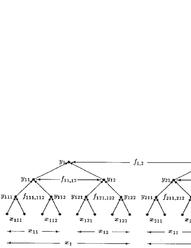
Figure 1: Notation used in the hierarchical maximum entropy derivation.

We shall apply the maximum entropy method with constraints of the form shown in Equation 5 to a hierarchy of transformed versions of the input vector $x$. In order to make our calculation tractable we introduce the notation shown in Figure 1. The $x_{ijk...}$ are various partitions of the input vector $x$, the $y_{ijk...}$ are various transformed versions $y_{ijk...}(x_{ijk...})$ of the input $x_{ijk...}$, and the $f_{ijk\cdots,i^{\prime}j^{\prime}k^{\prime}\cdots}$ are the Lagrange functions $f_{ijk\cdots,i^{\prime}j^{\prime}k^{\prime}\cdots}(y_{ijk\cdots},y_{i^{\prime}j^{\prime}k^{\prime}\cdots})$ that appear in the generalised version of the maximum entropy solution $Q_{\textup{mem}}(x)$ in  Equation 7.

We choose to write the dependence of $y_{ijk...}$ directly on the input $x_{ijk...}$, even though the value of $y_{ijk...}$ is obtained via a number of intermediate transformations leading from the leaf nodes of the tree up to node $ijk...$, because this leads to a transparent hierarchical maximum entropy derivation. It is convenient to define $\Pi_{ijk\cdots}(x_{ijk\cdots})$ as the product of the Lagrange functions that appear beneath node $ijk...$ of the tree. $\Pi_{ijk\cdots}(x_{ijk\cdots})$ has the following recursion property

$$\begin{array}[]{rl}\Pi_{ijk\cdots}\left(x_{ijk\cdots}\right)&=f_{ijk\cdots 1,ijk\cdots 2}(y_{ijk\cdots 1}(x_{ijk\cdots 1}),y_{ijk\cdots 2}(x_{ijk\cdots 2}))\\ &\begin{array}[]{cc}&\end{array}\times\Pi_{ijk\cdots 1}(x_{ijk\cdots 1})\Pi_{ijk\cdots 2}(x_{ijk\cdots 2})\end{array}$$ (12)

Also introduce a normalisation (or Jacobian) factor defined as

$$Z_{ijk\cdots}(y_{ijk\cdots})=\int dx_{ijk\cdots}\delta(y_{ijk\cdots}-y_{ijk\cdots}(x_{ijk\cdots}))\Pi_{ijk\cdots}(x_{ijk\cdots})$$ (13)

which is a sum of $\Pi_{ijk\cdots}(x_{ijk\cdots})$ over all the states $x_{ijk\cdots}$ of the leaf nodes beneath node $ijk...$ that are consistent with $y_{ijk...}$ emerging at node $ijk...$.

The proof of the general hierarchical maximum entropy result proceeds inductively. Firstly, we generalise Equation 4 to become

$$\begin{array}[]{rl}y_{i}(x)&\longrightarrow\delta\left(y_{ijk\cdots 1}-y_{ijk\cdots 1}(x_{ijk\cdots 1})\right)\delta(y_{ijk\cdots 2}-y_{ijk\cdots 2}(x_{ijk\cdots 2}))\\ \lambda_{i}&\longrightarrow\lambda_{ijk\cdots}(y_{ijk\cdots 1},y_{ijk\cdots 2})\end{array}$$ (14)

Secondly, we generalise Equation 8 to become

$$Q_{\textup{mem}}(x)=Q_{0}(x)f_{1,2}(y_{1}(x_{1}),y_{2}(x_{2}))\Pi_{1}(x_{1})\Pi_{2}(x_{2})$$ (15)

where we display the Lagrange function $f_{1,2}(y_{1},y_{2})$ that connects the topmost node-pair (i.e. node-pair $(1,2)$) in the tree, but conceal the other Lagrange functions by using the $\Pi_{ijk\cdots}$ notation.

We may determine the exact form of $f_{1,2}(y_{1},y_{2})$ independently of the rest of the Lagrange functions (which are hidden inside the $\Pi_{1}(x_{1})$ and $\Pi_{2}(x_{2})$ functions) by imposing the constraint shown in Equation 5 and Equation 6 (as applied to node-pair $(1,2)$) to obtain

$$\begin{array}[]{rl}P_{1,2}(y_{1},y_{2})&=\int dx_{1}dx_{2}\delta(y_{1}-y_{1}(x_{1}))\delta(y_{2}-y_{2}(x_{2}))Q_{\textup{mem}}(x)\\ &=f_{1,2}(y_{1},y_{2})Z_{1}(y_{1})Z_{2}(y_{2})\end{array}$$ (16)

which yields

$$f_{1,2}(y_{1},y_{2})=\frac{P_{1,2}(y_{1},y_{2})}{Z_{1}(y_{1})Z_{2}(y_{2})}$$ (17)

Substituting this result back into Equation 15 yields

$$Q_{\textup{mem}}(x)=P_{1,2}(y_{1}(x_{1}),y_{2}(x_{2}))\frac{\Pi_{1}(x_{1})}{Z_{1}(y_{1}(x_{1}))}\frac{\Pi_{2}(x_{2})}{Z_{2}(y_{2}(x_{2}))}$$ (18)

which correctly obeys the constraint on the joint PDF $P_{1,2}(y_{1},y_{2})$ of the topmost pair of nodes in the tree.

We now marginalise $Q_{\textup{mem}}(x)$ in order to concentrate our attention on the left-hand main branch of the tree. Thus

$$\begin{array}[]{rl}Q_{1,\textup{mem}}(x_{1})&=\int dx_{2}Q_{\textup{mem}}(x)\\ &=\int dx_{2}dy_{2}\delta(y_{2}-y_{2}(x_{2}))Q_{\textup{mem}}(x)\\ &=P_{1}(y_{1}(x_{1}))\frac{\Pi_{1}(x_{1})}{Z_{1}(y_{1}(x_{1}))}\end{array}$$ (19)

We now use the recursion property given in Equation 12 to extract the Lagrange function associated with node-pair $(11,12)$. Thus $Q_{1,\textup{mem}}(x_{1})$ becomes

$$Q_{1,\textup{mem}}(x_{1})=P_{1}(y_{1}(x_{1}))f_{11,12}(y_{11}(x_{11}),y_{12}(x_{12}))\frac{\Pi_{11}(x_{11})\Pi_{12}(x_{12})}{Z_{1}(y_{1}(x_{1}))}$$ (20)

As before, we may determine the exact form of $f_{11,12}(y_{11},y_{12})$ independently of the rest of the Lagrange functions by applying the constraints to node-pair $(11,12)$ to obtain

$$f_{11,12}(y_{11},y_{12})=\frac{P_{11,12}(y_{11},y_{12})}{P_{1}(y_{1})}\frac{Z_{1}(y_{1})}{Z_{11}(y_{11})Z_{12}(y_{12})}$$ (21)

where the value of $y_{1}$ is to be understood to be obtained directly from the values of $y_{11}$ and $y_{12}$ via the mapping which connects node-pair $(11,12)$ to node 1. Substituting this result into Equation 20 yields

$$Q_{1,\textup{mem}}(x_{1})=P_{11,12}(y_{11}(x_{11}),y_{12}(x_{12}))\frac{\Pi_{11}(x_{11})}{Z_{11}(y_{11}(x_{11}))}\frac{\Pi_{12}(x_{12})}{Z_{12}(y_{12}(x_{12}))}$$ (22)

By inspection, we see that Equation 18 and Equation 22 are identical in form once we have accounted for their different positions in the tree, so we may use induction to obtain all of the rest of the Lagrange functions in the form

$$\begin{array}[]{rl}f_{ijk\cdots 1,ijk\cdots 2}\left(y_{ijk\cdots 1},y_{ijk\cdots 2}\right)&=\frac{P_{ijk\cdots 1,ijk\cdots 2}(y_{ijk\cdots 1},y_{ijk\cdots 2})}{P_{ijk\cdots}(y_{ijk\cdots})}\\ &\begin{array}[]{cc}&\end{array}\times\frac{Z_{ijk\cdots}(y_{ijk\cdots})}{Z_{ijk\cdots 1}(y_{ijk\cdots 1})Z_{ijk\cdots 2}(y_{ijk\cdots 2})}\end{array}$$ (23)

which is analogous to Equation 21, and where $y_{\textup{ijk}\cdots}$ is obtained directly from the values of $y_{ijk\cdots 1}$ and $y_{ijk\cdots 2}$. The $\frac{\Pi}{Z}$ factors may be discarded once we reach the leaf nodes of the tree, because the integral in Equation 13 then reduces to $Z=\Pi$.

Finally, by starting with Equation 15 and recursively simplifying the $\Pi_{\textup{ijk}\cdots}$ using Equation 12 and substituting for the Lagrange functions $f_{ijk\cdots,i^{\prime}j^{\prime}k^{\prime}\cdots}$ using Equation 23 we obtain eventually for an $n$-layer tree

$$\begin{array}[]{rl}Q_{\textup{mem}}(x)&=\left[\prod\limits_{k=0}^{n-2}\prod\limits_{i_{1},i_{2},\cdots,i_{k}=1}^{2}\frac{P_{i_{1}i_{2}\cdots i_{k}1,i_{1}i_{2}\cdots i_{k}2}(y_{i_{1}i_{2}\cdots i_{k}1}(x_{i_{1}i_{2}\cdots i_{k}1}),y_{i_{1}i_{2}\cdots i_{k}2}(x_{i_{1}i_{2}\cdots i_{k}2}))}{P_{i_{1}i_{2}\cdots i_{k}1}(y_{i_{1}i_{2}\cdots i_{k}1}(x_{i_{1}i_{2}\cdots i_{k}1}))P_{i_{1}i_{2}\cdots i_{k}2}(y_{i_{1}i_{2}\cdots i_{k}2}(x_{i_{1}i_{2}\cdots i_{k}2}))}\right]\\ &\begin{array}[]{cc}&\end{array}\times\left[\prod\limits_{i_{1},i_{2},\cdots,i_{k}=1}^{2}P_{i_{1}i_{2}\cdots i_{n}}(x_{i_{1}i_{2}\cdots i_{n}})\right]\end{array}$$ (24)

where we have rearranged the terms to collect together the factors that each node-pair $(i_{1}i_{2}\cdots i_{k}1,i_{1}i_{2}\cdots i_{k}2)$ contributes.

Although we have concentrated on deriving $Q_{\textup{mem}}(x)$ for a binary tree, the principle of the derivation carries over unchanged to arbitrary tree structures, and Equation 24 may easily be generalised. In Appendix B we explain the relationship of the single layer version of Equation 24 to the random access memory network that is known as WISARD [15].

2.3 Diagrammatic notation

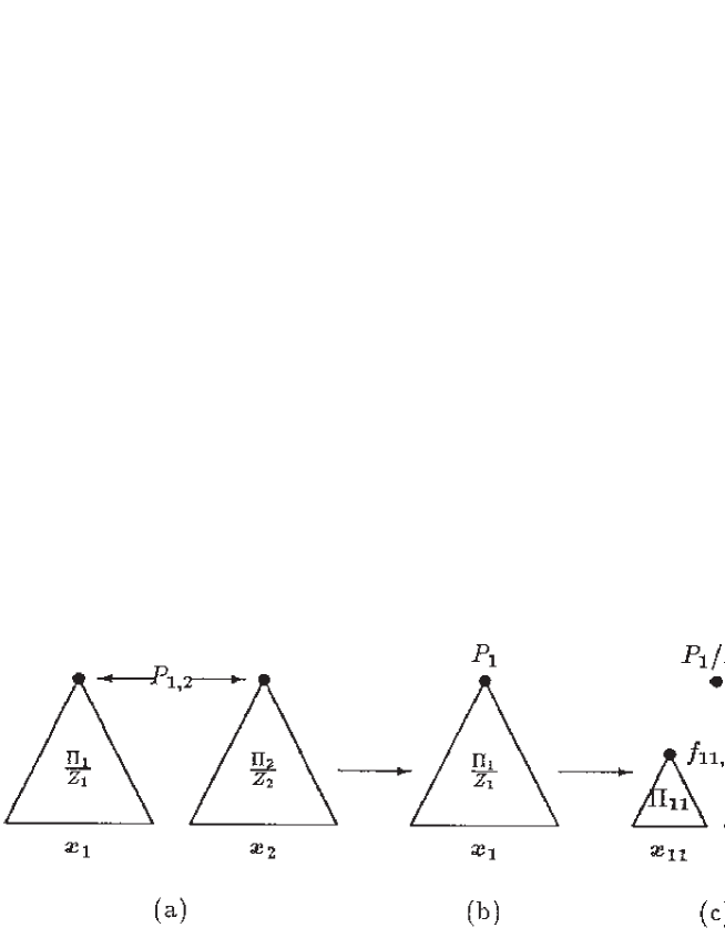
Figure 2: The individual steps of the inductive hierarchical maximum entropy derivation.

We now present the steps in the inductive derivation leading from Equation 18 to Equation 22 as a diagram in Figure 2. We use a triangle to represent a subtree, and we indicate its apex node, its associated $\Pi$ or $\frac{\Pi}{Z}$ factor, and its dependence on $x$. Figure 2a represents Equation 18, which is a pair of trees connected by the joint PDF of their apex nodes. By integrating over $x_{2}$ we remove the right hand tree to obtain Figure 2b, which corresponds to Equation 19. We then explicitly display the two daughter nodes to obtain Figure 2c, which corresponds to Equation 20, although we have grouped the terms together slightly differently, for simplicity. This exposes one of the Lagrange functions which we determine explicitly to obtain Figure 2d, which corresponds to Equation 22. One cycle of the inductive proof is completed by noting the correspondence between Figure 2a and Figure 2d.

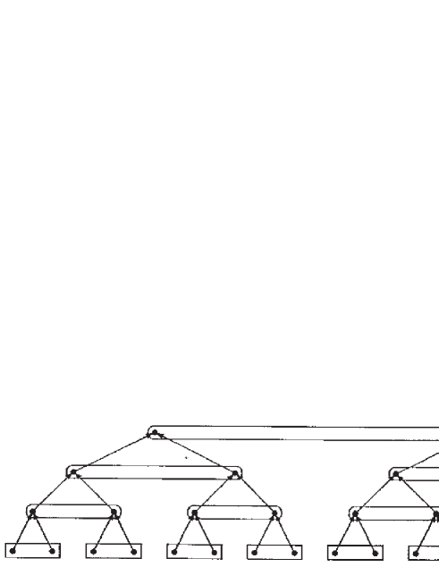
Figure 3: A diagrammatic representation of the hierarchical maximum entropy result.

We represent Equation 24 in diagrammatic form in Figure 3. The tree structure represents the flow of the transformations of the original input data $x$. Each square cornered rectangle represents the marginal PDF of the enclosed node-pair (i.e. one $P_{i_{1}i_{2}\cdots i_{n}}$ term from the second factor in Equation 24). Each round cornered rectangle represents the normalised marginal PDF of the encosed node-pair (i.e. one $\frac{P_{i_{1}i_{2}\cdots i_{k}1,i_{1}i_{2}\cdots i_{k}2}}{P_{i_{1}i_{2}\cdots i_{k}1}P_{i_{1}i_{2}\cdots i_{k}2}}$ term from the first factor in Equation 24). Overall, we obtain Equation 24 as the product of the rectangles in Figure 3.

This notation makes it easy to generalise the result in Equation 24 in a purely diagrammatic fashion, by firstly constructing an arbitrary (i.e. not necessarily binary) tree-like transformation of the input data, and secondly using as maximum entropy constraints the marginal PDF of each set of sister nodes in the tree. This prescription permits many possible ACE structures, including those in which different constraints effectively operate between different layers of the hierarchy (by mapping one or more node values directly from layer to layer).

Each rectangle representing a marginal PDF in Figure 3 contributes to the maximum entropy estimate of the PDF of a cluster of nodes in the input data. Because of the tree structure, clusters at each length scale are built out of clusters at smaller length scales. Equation 24 tells us exactly how to incorporate into $Q_{\textup{mem}}(x)$ any additional statistical properties that might be observed when forming larger clusters out of smaller clusters in this way.

Finally, Figure 3 suggests an informal derivation of Equation 24. Thus the expression for the maximum entropy estimate of the joint PDF of the input data $x$ in Equation 18 can be viewed as the joint PDF of the pair of nodes at the top of the tree in Figure 3 times corrective Jacobian factors that compensate for effects of the many-to-one mapping that the input data undergoes before it reaches the top of the tree. The final maximum entropy expression in Equation 24 merely enumerates these corrective Jacobian factors explicitly in terms of marginal PDFs measured at various levels of the tree. This makes it clear that the maximum entropy method gives a result that is consistent with simple counting arguments, which could therefore be used in place of the rather involved maximum entropy derivation.

3 Implementation of an anomaly detector

Henceforth we shall refer to our hierarchical maximum entropy method as an adaptive cluster expansion (ACE). In this section we describe how to implement Equation 24 in software. We assume that the ACE transformation functions have already been optimised using the unsupervised network training algorithm that we describe in Appendix A and in [13], so the purpose of this section is to explain how to manipulate Equation 24 into a form that produces a useful output from the network. For concreteness, we produce an output in the form of an image that represents the degree to which each local patch of an input data is statistically anomalous, when compared to the global statistical properties of the input data.

3.1 Two-dimensional array of inputs

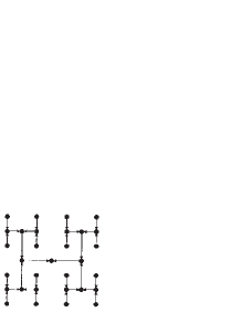
Figure 4: ACE connectivity for processing a 2-dimensional array of inputs.

In Section 2 we represented ACE as if it were operating on a 1-dimensional arrays of inputs (e.g. time series). In practice this might indeed be the case, but in this paper we choose to study 2-dimensional arrays of inputs (e.g. images). There is no difficulty in applying ACE to an image, provided that we appropriately assign the leaf nodes to pixels of the image. In Figure 4 we show the simplest possibility in which the image is alternately compressed in the north-south and east-west directions. A priori, the choice of whether to start with  north-south or east-west compression is arbitrary, but if we knew, for instance, that the image had stronger short range correlations in the east-west direction than the north-south direction, then it would be better to compress east-west first of all. Note that in Figure 4 the topology of the tree is the same as in Figure 3, but the way in which the leaf nodes are identified with the data samples is different.

More generally, we could identify the leaf nodes of the tree with the image pixels in any way that we please, provided that no pixel is used more than once (to guarantee that the tree-like topology is preserved). The problem of optimising the identification of leaf nodes with pixels is extremely complicated, so we shall not pursue it in this paper.

3.2 Histograms

The maximum entropy PDF in Equation 24 is a product of (normalised) marginal PDFs. In a practical implementation of ACE the $y_{ijk\cdots}$ are discrete-valued quantities (for instance, integers in the interval $[0,255]$), and the $P_{ijk\cdots,i^{\prime}j^{\prime}k^{\prime}\cdots}(y_{ijk\cdots},y_{i^{\prime}j^{\prime}k^{\prime}\cdots})$ are probabilities (not PDFs). We estimate the $P_{ijk\cdots,i^{\prime}j^{\prime}k^{\prime}\cdots}(y_{ijk\cdots},y_{i^{\prime}j^{\prime}k^{\prime}\cdots})$ by constructing 2-dimensional histograms

$$P_{ijk\cdots,i^{\prime}j^{\prime}k^{\prime}\cdots}(y_{ijk\cdots},y_{i^{\prime}j^{\prime}k^{\prime}\cdots})\simeq\frac{1}{N_{ijk\cdots,i^{\prime}j^{\prime}k^{\prime}\cdots}}h_{ijk\cdots,i^{\prime}j^{\prime}k^{\prime}\cdots}(y_{ijk\cdots},y_{i^{\prime}j^{\prime}k^{\prime}\cdots})$$ (25)

where $h_{ijk\cdots,i^{\prime}j^{\prime}k^{\prime}\cdots}(y_{ijk\cdots},y_{i^{\prime}j^{\prime}k^{\prime}\cdots})$ is the number of counts in the histogram bin $(y_{ijk\cdots},y_{i^{\prime}j^{\prime}k^{\prime}\cdots})$, and $N$ is the total number of histogram counts given by

$$N_{ijk\cdots,i^{\prime}j^{\prime}k^{\prime}\cdots}=\sum\limits_{y_{ijk\cdots}}\sum\limits_{y_{i^{\prime}j^{\prime}k^{\prime}\cdots}}h_{ijk\cdots,i^{\prime}j^{\prime}k^{\prime}\cdots}(y_{ijk\cdots},y_{i^{\prime}j^{\prime}k^{\prime}\cdots})$$ (26)

Note that the estimate in Equation 25 suffers from Poisson noise due to the finite number of counts in each histogram bin.

In order to build up this estimate we first of all train the ACE transformation functions as explained in Appendix A. The histogram bins are then initialised to zero, and subsequently filled with counts by exposing the trained ACE to many examples of input vectors (possibly, the set used to train the transformation functions). Thus each vector is propagated up through the ACE-tree, and we then inspect each node-pair $(ijk\cdots,i^{\prime}j^{\prime}k^{\prime}\cdots)$ for which a marginal probability needs to be estimated, and increment its corresponding histogram bin thus

$$h_{ijk\cdots,i^{\prime}j^{\prime}k^{\prime}\cdots}(y_{ijk\cdots},y_{i^{\prime}j^{\prime}k^{\prime}\cdots})\longrightarrow h_{ijk\cdots,i^{\prime}j^{\prime}k^{\prime}\cdots}(y_{ijk\cdots},y_{i^{\prime}j^{\prime}k^{\prime}\cdots})+1$$ (27)

When the training set has been exhausted, histogram bin $(ijk\cdots,i^{\prime}j^{\prime}k^{\prime}\cdots)$ records the number of times that state $(y_{ijk\cdots},y_{i^{\prime}j^{\prime}k^{\prime}\cdots})$ occurred.

A major disadvantage of using histograms is that they have a large number of adjustable parameters (i.e. the number of counts in each bin) that have to be determined by the training data, so they do not generalise very well. However, for the purpose of this paper, we do not need to resort to using more sophisticated ways of estimating PDFs.

3.3 Translation invariant processing

We wish to detect statistical anomalies in images which have otherwise spatially homogeneous statistics, such as textures. An invariance of the statistical properties of the true PDF $P(x)$ can be expressed as

$$P({\mathcal{G}}x)=P(x)$$ (28)

where ${\mathcal{G}}$ is any element of the invariance group, which we shall assume to be the group of translations of the image pixels. In Equation 24 $Q_{\textup{mem}}(x)$ does not respect translation invariance for two reasons. Firstly, we use transformations $y_{ijk\cdots}(x_{ijk\cdots})$ that are explicitly translation variant, because the functional form depends on the $ijk\cdots$ indices. Secondly, we connect together these transformations in translation variant way, because the tree structure in Figure 1 and Figure 4 does not treat all of its leaf nodes equivalently. We shall therefore modify the cluster expansion procedure that we derived in Section 2.2 to guarantee translation invariance. This will lead to a much improved maximum entropy estimate $Q_{\textup{mem}}(x)$ of the true $P(x)$.

Firstly, use the same transformation function at each position within a single layer of ACE. Thus in Equation 24 we make the replacement

$$\begin{array}[]{rl}y_{i_{1}i_{2}\cdots i_{k}1}(x_{i_{1}i_{2}\cdots i_{k}1})&\longrightarrow y^{k}(x_{i_{1}i_{2}\cdots i_{k}1})\\ y_{i_{1}i_{2}\cdots i_{k}2}(x_{i_{1}i_{2}\cdots i_{k}2})&\longrightarrow y^{k}(x_{i_{1}i_{2}\cdots i_{k}2})\end{array}$$ (29)

where we indicate that the transformation is associated with the $k$-th layer of ACE by attaching a superscript $k$ to each function. This yields

$$\begin{array}[]{rl}Q_{\textup{mem}}(x)&=\left[\prod\limits_{k=0}^{n-2}\prod\limits_{i_{1},i_{2},\cdots,i_{k}=1}^{2}\frac{P_{i_{1}i_{2}\cdots i_{k}1,i_{1}i_{2}\cdots i_{k}2}(y^{k}(x_{i_{1}i_{2}\cdots i_{k}1}),y^{k}(x_{i_{1}i_{2}\cdots i_{k}2}))}{P_{i_{1}i_{2}\cdots i_{k}1}(y^{k}(x_{i_{1}i_{2}\cdots i_{k}1}))P_{i_{1}i_{2}\cdots i_{k}2}(y^{k}(x_{i_{1}i_{2}\cdots i_{k}2}))}\right]\\ &\begin{array}[]{cc}&\end{array}\times\left[\prod\limits_{i_{1},i_{2},\cdots,i_{k}=1}^{2}P_{i_{1}i_{2}\cdots i_{n}}(x_{i_{1}i_{2}\cdots i_{n}})\right]\end{array}$$ (30)

Equation 30 guarantees translation invariance (in the sense of a “single-instruction-multiple-data” computer) of the processing that occurs when the input data is propagated upwards through the overlapping trees.

Secondly, assume that Equation 28 holds for all image translations, so that the marginal PDFs are independent of position. We may make this explicit in our notation by making the following replacement in Equation 30

$$\begin{array}[]{rl}\frac{P_{i_{1}i_{2}\cdots i_{k}1,i_{1}i_{2}\cdots i_{k}2}(\cdot)}{P_{i_{1}i_{2}\cdots i_{k}1}(\cdot)P_{i_{1}i_{2}\cdots i_{k}2}(\cdot)}&\longrightarrow\frac{P_{1,2}^{k}(\cdot)}{P_{1}^{k}(\cdot)P_{2}^{k}(\cdot)}\\ P_{i_{1}i_{2}\cdots i_{n}}(\cdot)&\longrightarrow P^{n-1}(\cdot)\end{array}$$ (31)

where we use the same superscript notation as in Equation 29. This yields

$$\begin{array}[]{rl}Q_{\textup{mem}}(x)&=\left[\prod\limits_{k=0}^{n-2}\prod\limits_{i_{1},i_{2},\cdots,i_{k}=1}^{2}\frac{P_{1,2}^{k}(y^{k}(x_{i_{1}i_{2}\cdots i_{k}1}),y^{k}(x_{i_{1}i_{2}\cdots i_{k}2}))}{P_{1}^{k}(y^{k}(x_{i_{1}i_{2}\cdots i_{k}1}))P_{2}^{k}(y^{k}(x_{i_{1}i_{2}\cdots i_{k}2}))}\right]\\ &\begin{array}[]{cc}&\end{array}\times\left[\prod\limits_{i_{1},i_{2},\cdots,i_{k}=1}^{2}P^{n-1}(x_{i_{1}i_{2}\cdots i_{n}})\right]\end{array}$$ (32)

Equation 32 guarantees not only translation invariance of the transformations that propagate the data through the tree, but also translation invariance of the marginal PDFs of $P(x)$ that are used to construct $Q_{\textup{mem}}(x)$.

Both of the simplifications in Equation 29 and Equation 31 reduce the total number of unknowns that have to be determined. For a given amount of training data we can thus construct a better maximum entropy estimate $Q_{\textup{mem}}(x)$ of the true P(x). The transformation functions may be optimised better, and the histogram bins have a reduced Poisson noise.

We usually apply ACE to such large input arrays that it is not appropriate to build a single binary tree whose leaf nodes encompass the entire input array. Instead, we divide the input array (which we shall assume is a $2^{M}\times 2^{M}$ array of image pixels) into a set of contiguous $2^{m_{1}}\times 2^{m_{2}}$ arrays, each of which we analyse using Equation 32. There are no constraint functions to measure the mutual dependencies between these subarrays, so the maximum entropy joint PDF of the set of subarrays is a product of terms of the form shown in Equation 32.

$$\begin{array}[]{rl}\log(Q_{\textup{mem}}(x))&=\sum\limits_{k=0}^{n-2}\sum\limits_{a_{1}=1}^{2^{M-m_{1}}}\sum\limits_{a_{2}=1}^{2^{M-m_{2}}}\sum\limits_{i_{1},i_{2},\cdots,i_{k}=1}^{2}\log(\frac{P_{1,2}^{k}(y^{k}(x_{i_{1}i_{2}\cdots i_{k}1}^{a_{1},a_{2}}),y^{k}(x_{i_{1}i_{2}\cdots i_{k}2}^{a_{1},a_{2}}))}{P_{1}^{k}(y^{k}(x_{i_{1}i_{2}\cdots i_{k}1}^{a_{1},a_{2}}))P_{2}^{k}(y^{k}(x_{i_{1}i_{2}\cdots i_{k}2}^{a_{1},a_{2}}))})\\ &\begin{array}[]{cc}&\end{array}+\log\left(\sum\limits_{a_{1}=1}^{2^{M-m_{1}}}\sum\limits_{a_{2}=1}^{2^{M-m_{2}}}\sum\limits_{i_{1},i_{2},\cdots,i_{k}=1}^{2}\log(P^{n-1}(x_{i_{1}i_{2}\cdots i_{n}}^{a_{1},a_{2}}))\right)\end{array}$$ (33)

The summation over $(a_{1},a_{2})$ ranges over the $2^{2M-m_{1}-m_{2}}$ contiguous subarrays in the overall $2^{M}\times 2^{M}$ array, and the $a_{1},a_{2}$ superscript on each $x_{ijk\cdots}$ vector indicates that it belongs to subarray $(a_{1},a_{2})$. Note that we have transformed $Q_{\textup{mem}}(x)\longrightarrow\log(Q_{\textup{mem}}(x))$ for convenience.

The final step in constructing a fully translation invariant PDF is to modify the sum over subarrays so that it includes all possible placements of the $2^{m_{1}}\times 2^{m_{2}}$ subarray within the overall $2^{M}\times 2^{M}$ array. There are $2^{2M-m_{1}-m_{2}}$ possible positions when the placement of the subarray is restricted as in Equation 33, whereas there are $(2^{M}-2^{m_{1}}+1)(2^{M}-2^{m_{2}}+1)$ possible positions when all placements of the subarray are permitted. We therefore make the replacement

$$\begin{array}[]{rl}\sum\limits_{a_{1}=1}^{2^{M-m_{1}}}\sum\limits_{a_{2}=1}^{2^{M-m_{2}}}\left(\cdot\right)&\longrightarrow\frac{2^{2M-m_{1}-m_{2}}}{\left(2^{M}-2^{m_{1}}+1\right)\left(2^{M}-2^{m_{2}}+1\right)}\sum\limits_{p_{1}=1}^{2^{M}-2^{m_{1}}+1}\sum\limits_{p_{2}=1}^{2^{M}-2^{m_{2}}+1}\left(\cdot\right)\\ &\simeq 2^{-m_{1}-m_{2}}\sum\limits_{p_{1}=1}^{2^{M}}\sum\limits_{p_{2}=1}^{2^{M}}\left(\cdot\right)\end{array}$$ (34)

in Equation 33, where $(p_{1},p_{2})$ is the coordinate of the pixel in the top left hand corner of the $2^{m_{1}}\times 2^{m_{2}}$ subarray. If we ignore edge effects, then we may use the approximation in the final line of Equation 34, which is the average of $2^{m_{1}+m_{2}}$ separate contributions of the form shown in Equation 33. Equation 34 effectively replaces the original maximum entropy PDF $Q_{\textup{mem}}(x)$ by the geometric mean of a set of maximum entropy PDFs. This averaging reduces the problems caused by Poisson noise on the histogram bin contents to yield a greatly improved maximum entropy PDF estimate.

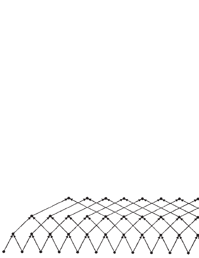
Figure 5: Connectivity for multiple overlapping binary trees.

In practice, we would implement each layer of ACE as a frame store, and the transformation between each pair of adjacent layers as a look-up table. The translation invariant ACE that we derived in Equation 33 (with the replacement given in Equation 34) may be implemented using the connectivity shown in Figure 5. Ignoring edge effects, we may write Equation 33 symbolically as

$$\log(Q_{\textup{mem}}(x))\simeq\sum\limits_{k=0}^{n-2}\frac{1}{2^{n-k}}\sum\log(\frac{P_{1,2}^{k}}{P_{1}^{k}P_{2}^{k}})+\frac{1}{2}\sum\log(P^{n-1})$$ (35)

where the inner summations range over all positions within a single layer of Figure 5. We omit all of the functional dependencies, because they are easy to obtain from Figure 3. Each $\frac{P_{1,2}^{k}}{P_{1}^{k}P_{2}^{k}}$ term is represented by a rectangle with rounded corners in Figure 3, and each $P^{n-1}$ term is represented by a rectangle with square corners in Figure 3. We have not drawn these rectangles in Figure 5 because they would overlap, and thus confuse the diagram.

3.4 Forming a probability image

Equation 35 is the fundamental result that we use to construct useful image processing schemes. However, it would not be very useful simply to calculate the value of $\log(Q_{\textup{mem}})$ as a single global measure of the logarithmic probability associated with an image. We choose instead to break up Equation 35 into smaller pieces, and to examine their contribution to the overall $\log(Q_{\textup{mem}})$. In effect, we look at how $\log(Q_{\textup{mem}})$ is built up from the information in each layer of ACE, which in turn we break down into contributions from different areas of the image.

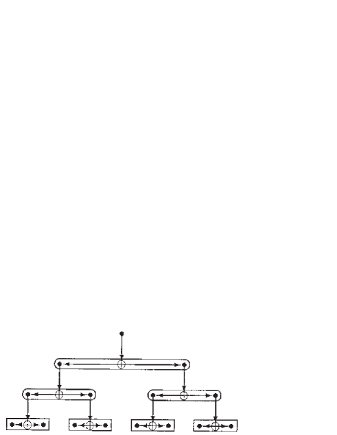
Figure 6: Backpropagation scheme for constructing a probability image.

In order to ensure that our decomposition of $\log(Q_{\textup{mem}})$ can be easily computed, we use the backpropagation scheme shown in Figure 6 to control the data flow through a translation invariant network of an identical connectivity to the one shown in Figure 5. Each node of this backpropagation network records a logarithmic probability, and is cleared to zero before starting the backpropagation computations. The rectangles in Figure 6 represent exactly the same logarithmic probability terms that appeared in Figure 3, which we now use as sources of logarithmic probability that we inject into the backpropagating data flow.

The detailed operation of Equation 30 is as follows. Each addition symbol takes as input a contribution recorded at a node in the next layer above, adds its own logarithmic probability source $\log(\frac{P_{1,2}^{k}}{P_{1}^{k}P_{2}^{k}})$, scales the result by $\frac{1}{4}$, and it finally adds a copy of this result to the value stored at each of its own pair of associated nodes, as shown. The values that accumulate at the leaf nodes represent various contributions to the sum in Equation 35. If the translation invariant version of Figure 6 is applied to the translation invariant network shown in Figure 5, then the sum of the values that accumulate at the leaf nodes reproduces Equation 35 precisely.

This method of computing $\log(Q_{\textup{mem}})$ might seem to be circuitous, but it has the great advantage of both being computationally cheap and forming an image-like representation of $\log(Q_{\textup{mem}})$, which we call a “probability image”. Each $\log(\frac{P_{1,2}^{k}}{P_{1}^{k}P_{2}^{k}})$ term in Equation 35 will contribute equally to $2^{n-k}$ pixels in the probability image. These pixels will be arranged as either a square or a 2-to-1 aspect ratio rectangle according to whether there is an odd number or even number of backpropagation steps from the k-th layer to the leaf nodes. The probability image is therefore a superposition of square and rectangular tiles of logarithmic probability. Each tile corresponds to a node of the network shown in Figure 5.

It is useful to display as an image the contributions of a single layer of the network to the probability image, because different layers contribute to the structure of $\log(Q_{\textup{mem}})$ at different length scales. This image may be displayed in the conventional way, with small probabilities mapped to black, large probabilities mapped to white, and intervening probabilities mapped to shades of grey, in which case we call it a “probability image”. It is also useful to invert the grey scale so that small probabilities map to black, in which case we call it an “anomaly image”, because regions which have statistical properties that occur infrequently show up as bright peaks in the image. We find that the use of probability images and/or anomaly images is an extremely effective way of visually interpreting $\log(Q_{\textup{mem}})$ in Equation 35.

3.5 Modular implementation

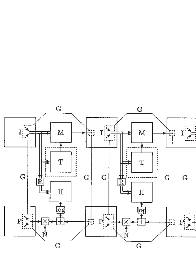
Figure 7: Three layer translation invariant ACE system.

For completeness we now present a brief description of a complete system for producing probability and/or anomaly images. This system consists of two tightly coupled subsystems - an ACE subsystem for decomposing the image data, and a probability image subsystem for forming the output image. Figure 7 combines in one diagram all of the results that we have discussed so far. The upper part of Figure 7 is a pure translation invariant ACE subsystem, whereas the lower half is a backpropagating probability image subsystem operating as shown in Figure 6. The backpropagating subsystem takes input information from various layers of ACE, as shown. Modules “I” are framestores that record the various transformed images. Modules “M” are look-up tables that record the inter-layer mappings. Modules “T” represent the training algorithm that we explain in Appendix A, which we enclose in a dashed box because the “T” modules are switched out of the circuit once the mappings “M” have been determined. Modules “H” are accumulators that record the 2-dimensional histograms, and then regularise and normalise them appropriately. Modules “P” are framestores that record the various backpropagated probability images. Modules “log” are look-up tables (in fact only one such table is needed) that implement a logarithm function. Modules “$\oplus\ \$” and “$\otimes\ \$” perform the addition and scaling operations that we discussed earlier in connection with Figure 6. “N” is scaling factor (which is $\frac{1}{4}$ if we wish to reproduce the result in Equation 35). The lines that are annotated “G” represent a ganging together of the (pointers to) pixels in adjacent layers of the ACE subsystem and in the probability image subsystem. These ensure that the entire system works in lockstep, as required.

The simplest mode of operation of this system can be broken down into three stages Firstly, train each layer (from left to right) of the ACE subsystem on a training image. Secondly, propagate a test image (from left to right) through the layers of ACE. Finally, construct a probability image by backpropagating (from right to left) contributions from the various layers of ACE. Furthermore, it is useful to display separately the probability (or anomaly) images that emerge from each layer of ACE, as we shall see in Section 4.

There is a variety of methods of optimising “T”, and hence “M”. The method that we describe in Appendix A trains each layer in sequence, which takes 2.3 second per layer (using a VAXstation 3100, and assuming 6 bits per pixel), which gives a full training time of 20 seconds for the 8 layer network that we use in our numerical simulations. We do not make use of more sophisticated schemes in which different layers are simultaneously trained, whilst communicating information with each other to improve the global performance of ACE.

3.6 Relationship to co-occurrence matrix methods

Both the basic maximum entropy PDF $Q_{\textup{mem}}(x)$ in Equation 24, and the translation invariant version of $\log(Q_{\textup{mem}}(x))$ in  Equation 35 that we implement in practice, depend on various PDFs that are measured in an ACE-tree. The second term of Equation 35 may be written as

$$Q_{\textup{mem}}(x)=\sqrt{\prod P^{n-1}}$$ (36)

Each $P^{n-1}$ factor is the spatial average of the marginal PDF of pairs of adjacent pixel values, assuming that we use the identification of leaf nodes with pixels that we show in Figure 4. The square root in Equation 36 compensates for the fact that the product of $P^{n-1}$ factors generates the product of two maximum entropy PDFs shifted by one pixel relative to each other.

By using Equation 25 we may approximate Equation 36 as a product of histograms. In this case each histogram is the spatial average of the co-occurrence matrix of pairs of adjacent pixel values, as commonly used in image processing [7]. Thus we may use conventional co-occurrence matrix methods to construct a simple form of maximum entropy PDF, which corresponds to using only one layer of ACE.

This co-occurrence matrix result can be generalised, using Equation 24 or Equation 35, to model higher order statistical behaviour. Although these results depend on co-occurrence matrices measured at various places in the ACE-tree, the contributions which do not depend directly on the input data (i.e. the first term of Equation 35) actually model higher order statistics of the input data. This is because the value $y_{ijk\cdots}$ that emerges from node $ijk\cdots$ of the ACE-tree depends on $x_{ijk\cdots}$, so the joint PDF $P_{ijk\cdots 1,ijk\cdots 2}(y_{ijk\cdots 1},y_{ijk\cdots 2})$ depends on the statistics of the pair $(x_{ijk\cdots 1},x_{ijk\cdots 2})$. Thus ACE is a very convenient way of combining together the various orders of statistical information that are contained in co-occurrence matrices at various places in the ACE-tree, as shown in Figure 3.

4 Numerical results

In this section we explain the finer details of how to implement Figure 7 in software, and we present the results of applying the system to four $256\times 256$ images of textiles taken from the Brodatz texture set [16].

4.1 Experimental procedure

We compensated for some of the effects of non-uniform illumination by adding to each image a grey scale wedge whose gradient was chosen in such a way as to remove the linear component of the non-uniformity. Not only does this improve the translation invariance of the image statistics, but it also improves the quality of the hierarchical coding of the image, because we reduce the need to develop redundant codes which differ only in their overall grey level.

Throughout our experiments we generate optimal inter-layer mappings using the training methods that we explain in Appendix A. These are known as topographic mappings in the neural network literature, and we showed in [19] why they are appropriate for building multistage vector quantisers. We choose to compress the image in alternate directions using the following sequence: north/south, east/west, north/south, east/west, etc. This compression sequence leads to the following sequence of rectangular image regions that influence the state of each pixel in each stage of ACE: $1\times 2$, $2\times 2$, $2\times 4$, $4\times 4$, etc, using (east/west, north/south) coordinates. In all of our experiments we use an 8 stage ACE.

The number of bits per pixel that we use in each layer of ACE determines the quality of the hierarchical vector quantisation that emerges. Increasing the number of bits improves the quality of the vector quantisation but increases the training time: we need to compromise between these two conflicting requirements. In our work on simple Brodatz texture images we have found that 6-8 bits per pixel is sufficient.

It is important to note that for a given number of bits (after compression) there is an upper limit on the allowed entropy that the input data can have. This problem becomes more severe the greater the data compression factor (i.e. the further we progress through the layers of ACE). For instance, if the input image is very noisy then 6-8 bits will be sufficient only to give good vector quantisation performance in the first few layers of ACE. This problem arises because ACE does not have much prior knowledge of the statistical properties of the input data, so each node of ACE encodes its input without assuming a prior model. A prior model would allow us to reduce the bit rate. This is a fundamental limitation to the capabilities of the current version of ACE.

The choice of the size of the 2-dimensional histogram bins is also important. A property of the topographic mappings that we use to to connect the layers of ACE is that adjacent histogram bins derive from input vectors that are close to each other (in the Euclidean sense), so it is sensible to rebin the histogram by combining together adjacent bins. Thus we control the histogram bin size by truncating the low order bits of each binary vector that represents a pixel value. If we do not truncate any bits, then the 2-dimensional histogram faithfully records the number of times that a pair of pixel values has occured. However, if we truncate $b$ low order bits of each pixel value then effectively we sum together the histogram bins in groups of $2^{2b}$ ($=2^{b}\times 2^{b}$) adjacent bins, which smooths the histogram. The more smoothing that we impose the less Poisson noise the histogram suffers. However, as we smooth the histogram we run the danger of smoothing away significant structure that might usefully be used to characterise the input image: so we need to make a compromise. In our Brodatz texture work we use only 4-6 bits of each pixel value to generate the histograms in each stage of ACE. Note that we use more bits for vector quantisation than for histogramming because the vector quantisation needs to be good enough to preserve information for encoding by later layers of the hierarchy, whereas the histogramming information is not passed to later layers.

In Equation 35 we need to estimate the logarithm of various probabilities from the histograms. We do this in two stages. Firstly, we regularise the histograms by placing a lower bound on the permitted number of counts. One possible prescription is to ensure that each histogram bin has a number of counts at least as large as the average number of counts in all the histogram bins (as determined before regularising the histogram). Thus

$$h_{ijk\cdots,i^{\prime}j^{\prime}k^{\prime}\cdots}(y_{ijk\cdots},y_{i^{\prime}j^{\prime}k^{\prime}\cdots})\longrightarrow\left\{\begin{array}[]{ccc}h_{ijk\cdots,i^{\prime}j^{\prime}k^{\prime}\cdots}(y_{ijk\cdots},y_{i^{\prime}j^{\prime}k^{\prime}\cdots})&&h\geq\left\langle h\right\rangle\\ \left\langle h_{ijk\cdots,i^{\prime}j^{\prime}k^{\prime}\cdots}(y_{ijk\cdots},y_{i^{\prime}j^{\prime}k^{\prime}\cdots})\right\rangle&&h<\left\langle h\right\rangle\end{array}\right.$$ (37)

where the angle brackets $\langle\cdots\rangle$ denote an average over histogram bins, rounded up to the next largest integer to avoid setting histogram bins to zero. Secondly, we estimate the probabilities $P_{ijk\cdots,i^{\prime}j^{\prime}k^{\prime}\cdots}(y_{ijk\cdots},y_{i^{\prime}j^{\prime}k^{\prime}\cdots})$ by inserting the regularised histograms into Equation 25. We use a marginalised version of Equation 25 to estimate the marginal probabilities $P_{ijk\cdots}(y_{ijk\cdots})$. Finally, we compute the logarithmic probabilities in Equation 35 by using a table of logarithms of integers, up to the maximum possible number of counts that could occur in a histogram bin - it suffices to tabulate logarithms up to $\log(N)$.

The prescription in Equation 37 is crude but effective. We could improve the performance by introducing prior knowledge of the statistical properties of the input data. Our histogram smoothing prescription already implicity makes use of prior knowledge of the properties of the Posson noise process that affects the histogram counts, and prior knowledge of the fact that adjacent histogram bins correspond to similar input vectors. Additional prior knowledge would further enhance the performance, especially in cases where there is a limited amount of training data (such as small images, or small segments of larger images).

A pitfall that must be avoided is using histogram bins that are too small when one intends to train ACE on one image and then use a different image to generate a probability image. Effectively, the large number of small bins records the details of the statistical fluctuations of the training image (as particular realisations of a Poisson noise process in each bin), which thus acts as a detailed record of the structure in the training image. The histograms thus look very spiky, and in an extreme case there may be a counts recorded in only a few bins with zeros in all of the remaining bins. If this situation occurs then the training image records a large $\log(Q_{\textup{mem}}(x))$, whereas a test image having the same statistical properties records a small $\log(Q_{\textup{mem}}(x))$. Effectively, the spikes in the training and test image histograms are not coincident. This problem can be solved by choosing a large enough histogram bin size.

Finally, we display the logarithmic probability image as follows. We determine the range of pixel values that occurs in the image, and we translate and scale this into the range $[0,255]$. This ensures that the smallest logarithmic probability appears as black, and the largest logarithmic probability appears as white, and all other values are linearly scaled onto intermediate levels of grey. This prescription has its dangers because each probability image determines its own special scaling, so one should be careful when comparing two different probability images. It can also be adversely affected by pixel value outliers arising from Poisson noise effects, where an extreme value of a single pixel could affect the way in which the whole of an image is displayed. However, we find that the overlapping tree prescription in Figure 5 together with the backpropagation prescription in Figure 6, causes enough effective averaging together of the histogram bins that we do not encounter problems with pixel value outliers.

In all of the images that we present below, we compensate for the uneven illumination by introducing a grey scale wedge as we explained earlier, we use 8 bits per pixel for vector quantisation, we use 6 bits per pixel for histogramming, and we invert the $[0,255]$ scale to produce an anomaly image, in which a white pixel indicates a small (rather than a large) logarithmic probability.

4.2 Texture 1

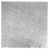
Figure 8: $256\times 256$ image of Brodatz fabric number 1.

In Figure 8 we show the first Brodatz texture image that we use in our experiments. The image is slightly unevenly illuminated and has a fairly low contrast, but nevertheless its statistical properties are almost translation invariant.

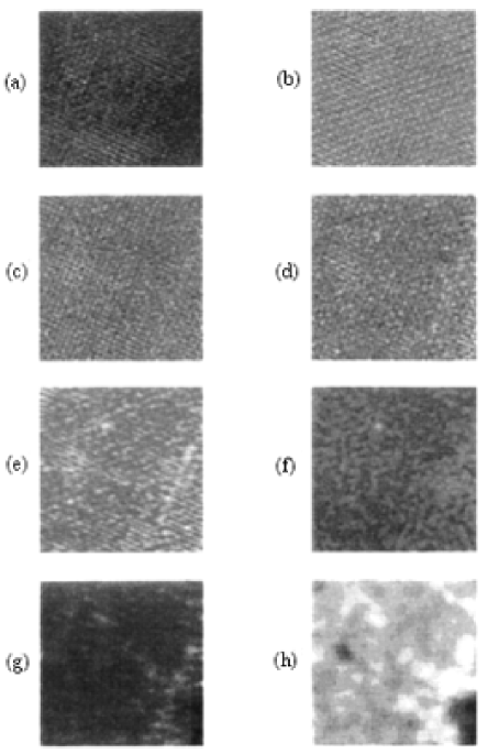
Figure 9: $256\times 256$ anomaly images of Brodatz fabric number 1.

In Figure 9 we show the anomaly images that derive from Figure 8. Note how the anomaly images become smoother as we progress from Figure 9a to Figure 9h, due to the increasing amount of averaging that occurs amongst the overlapping backpropagated rectangular tiles that build up each image.

Figure 9e and especially Figure 9f reveal a highly localised anomaly in the original image. Figure 9f corresponds to a length scale of $8\times 8$ pixels, which is the approximate size of the fault that is about $\frac{1}{4}$ of the way down and slightly to the left of centre of Figure 8. The fault does not show up clearly on the other figures in Figure 9 because their characteristic length scales are either too short or too long to be sensitive to the fault.

There is a major feature in the bottom right hand corner of Figure 9h, where the anomaly image is darker than average, indicating that the corresponding part of the original image has a higher than average probability. This is a different type of anomaly to the sort that we have envisaged so far - it occurs because the corresponding part of original image happens to explore only a high probability part of the space that is explored by the whole image. This part of the anomaly image is surrounded by a brighter than average border, which indicates a conventional anomalous region.

From Figure 9 we conclude that ACE can easily pick out localised faults in highly ordered textures.

4.3 Texture 2

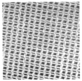
Figure 10: $256\times 256$ image of Brodatz fabric number 2.

In Figure 10 we show the second Brodatz texture image that we use in our experiments. The image has a high contrast and translation invariant statistical properties.

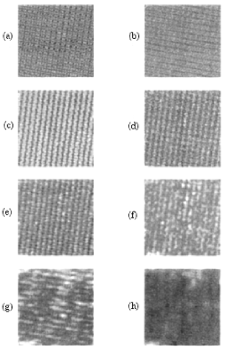
Figure 11: $256\times 256$ anomaly images of Brodatz fabric number 2.

In Figure 11 we show the anomaly images that derive from Figure 10. The most interesting anomaly image is Figure 11f which shows several localised anomalies. About halfway down and to the left of centre of the image is an anomaly that corresponds to a dark spot on the thread in Figure 10. The brightest of the anomalies in the cluster just above the centre of the image corresponds to what appears to be a slightly torn thread in Figure 10. The other anomalies in this cluster are weaker, and correspond to slight distortions of the threads. There is another anomaly just below and to the right of the centre of Figure 11g, which corresponds to what appears to be another slightly torn thread in Figure 10. These anomalies all occur at, or around, a length scale of $8\times 8$ pixels. Several of the anomaly images show an anomaly in the bottom left hand corner of the image, which corrsponds to a small uniform patch of fabric in Figure 10.

The results in Figure 11 corroborate the evidence in Figure 9 that ACE can be trained in an unsupervised fashion to pick out localised faults in highly ordered textures.

4.4 Texture 3

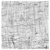
Figure 12: $256\times 256$ image of Brodatz fabric number 3.

In Figure 12 we show the third Brodatz texture image that use in our experiments.The image has a very high contrast and statistical properties that are almost translation invariant. However the density of anomalies is much higher than in either Figure 8 or Figure 10.

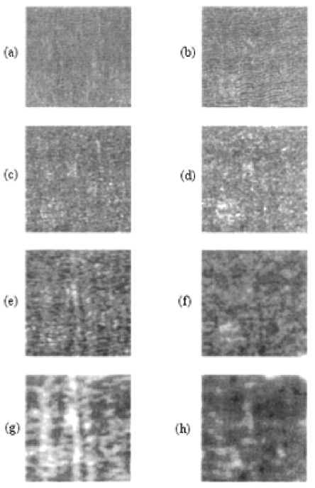
Figure 13: $256\times 256$ anomaly images of Brodatz fabric number 3.

In Figure 13 we show the anomaly images that derive from Figure 12. The most prominant anomaly is in Figure 13g, at a length scale of $8\times 16$ pixels, which corresponds to region of Figure 12 that is just above and to the left of centre of the image. This region is anomalous because it is both distorted and has slightly thicker threads than elsewhere. The large distorted region in the bottom left hand corner of Figure 12 does not show up very clearly to the naked eye in Figure 13, but Figure 13f and Figure 13h have significant peaks in this region. There are also many other localised peaks in Figure 13 which can be traced back to corresponding faults in Figure 12.

Comparing Figure 13 with Figure 9 and Figure 11 we conclude that the ability of ACE to pick out faults is degraded as the density of faults increases. This is because the faults themselves are part of the statistical properties that are extracted by ACE, and if a particular fault occurs often enough in the image then it is no longer deemed to be a fault.

4.5 Texture 4

In this section we present a slightly different type of experiment in which we train ACE on one image and test ACE on another image. To create the two images we start with a single $256\times 256$ image of a Brodatz texture, which we divide into a left half and a right half. We then use the left half to build up the training image, and the right half to build up the test image.

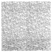
Figure 14: $256\times 256$ image of Brodatz carpet for training.

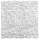
Figure 15: $256\times 256$ image of Brodatz carpet for testing.

In Figure 14 we show the training image which is a montage of two copies of the left hand half of a Brodatz texture image. Note that this montage contains only as much information as was present in the original half image from which it was constructed. In Figure 15 we show the test image which is a montage of two copies of the right hand half of a Brodatz texture image, and superimposed on that is a $64\times 64$ patch which we generated by flipping the rows and columns of a copy of the top left hand corner of this image. This patch is a hand crafted anomaly. Note that in constructing these images we have scrupulously avoided the possibility that the training and test images could contain elements deriving from a common source.

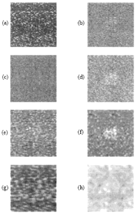
Figure 16: $256\times 256$ anomaly images of Brodatz carpet.

In Figure 16 we show the anomaly images that derive from Figure 15 after having trained on Figure 14. Figure 16f shows the strongest response to the anomalous patch in the centre of the image, corresponding to anomaly detection on a length scale of $8\times 8$ pixels.

5 Conclusions

Using maximum entropy methods, we have shown how to construct maximum entropy estimates of PDFs by using adaptive hierarchical transformation functions to record various marginal PDFs of the data, which we call an “Adaptive Cluster Expansion” (ACE). This method is a member of the same family as the trainable MRF known as the Boltzmann Machine, but it uses sophisticated transformations of the input data rather than hidden variables to characterise the high order statistical properties of the training set. The simulations in this paper use hierarchical topographic mappings to build these transformations, but this is a convenience, not a necessity.

We have also shown how to extend ACE so that it can be applied to translation invariant image processing, such as the detection of statistical anomalies in otherwise statistically homogeneous textures. Our methods show great promise, not only because they are amenable to a full theoretical analysis leading to closed-form maximum entropy solutions, but also because they lead directly to a modular system design which can locate anomalies in textures.

We have presented several examples where ACE successfully detects anomalous regions in otherwise statistically homogeneous textures. In all cases ACE adaptively extracts the global statistics of an image at various length scales during the unsupervised training, which takes 20 seconds (on a VAXStation 3100) for the 8 layer ACE network that we applied to this problem. ACE then uses these statistics to form an output image that represents the probability that each local patch of the input image belongs to the ensemble of patches presented during training. We call this a “probability image”.

Some possible applications of our results are as follows. Inspection of textiles: this relies on the assumed statistical homogeneity of an unflawed piece of textile, so that faults show up as anomalies, which we have demonstrated successfully in this paper. Detection of targets in noisy background clutter in radar images: this is basically a noisy version of the textile inspection problem, which goes somewhat beyond what we have presented in this paper, because it needs to address the problem of the noise entropy saturating ACE. Texture segmentation: this is an ambitious goal which requires much further analysis in order to derive a computationally cheap method of handling multiple simultaneous textures.

Appendix A Vector quantisation

In this appendix we summarise the hierarchical vector quantisation method that we presented in detail in [13]. In this paper we use this technique to optimise the inter-layer mappings in Figure 7. We have applied this technique elsewhere to image compression [20], and multilayer self-organising neural networks [10, 12, 19, 14].

A.1 Standard vector quantisation

This subsection contains those details of the theory of standard vector quantisation that one needs to understand before proceeding to the modified vector quantisation scheme that we present in Section A.2.

The problem is to form a coding $y$ of a vector $x$ in such a way that a good estimate $x^{\prime}$ of $x$ can be constructed from knowledge of $y$ alone. The sketch derivation in this section is presented in greater detail in [19]. Thus a vector quantiser is constructed by minimising a Euclidean distortion $D_{1}$ with respect to the choice of coding function $y(x)$ and decoding function $x^{\prime}(y)$, where

$$D_{1}=\int dxP(x)\left\|x-x^{\prime}(y(x))\right\|^{2}$$ (38)

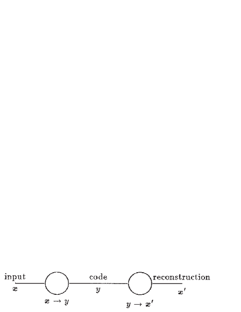
Figure 17: Encoding and decoding in a vector quantiser.

We may represent the encoding and decoding operations diagrammatically as shown in Figure 17. By functionally differentiating $D_{1}$ with respect to $y(x)$ and $x^{\prime}(y)$ we obtain

$$\frac{\delta D_{1}}{\delta y(x)} \left.=P(x)\frac{\partial}{\partial y}\left\|x^{\prime}(y)-x\right\|^{2}\right|_{y=y(x)}$$ (39)

$$\frac{\delta D_{1}}{\delta x^{\prime}(y)} =2\int dxP(x)\delta(y-y(x))\left(x^{\prime}(y)-x\right)$$ (40)

Setting $\frac{\delta D_{1}}{\delta y(x)}=0$ in Equation 39 yields the optimum encoding function

$$y(x)=\arg\begin{array}[]{c}\min\\ y\end{array}\left\|x-x^{\prime}(y(x))\right\|^{2}$$ (41)

which is called “nearest neighbour encoding”. Setting $\frac{\delta D_{1}}{\delta x^{\prime}(y)}=0$ in Equation 40 yields the optimum decoding function

$$x^{\prime}(y)=\frac{\int dxP(x)\delta(y-y(x))x}{\int dxP(x)\delta(y-y(x))}$$ (42)

which is the update scheme derived in [21]. Alternatively, we may use an incremental scheme to optimise the decoding function by following the path of steepest descent which we may obtain from Equation 40 as

$$\begin{array}[]{cc}\delta x^{\prime}(y)=\epsilon\delta(y-y(x))\left(x-x^{\prime}(y)\right)&\operatorname{where}0<\epsilon<1.\end{array}$$ (43)

An iterative optimisation scheme may be formed by alternately applying Equation 41 and then either Equation 42 or Equation 43. This scheme will alternately improve the encoding and decoding functions until a local minimum distortion is located. Alternating Equation 41 and Equation 42 is commonly called the “LBG” (after the authors of [21]) or “k-means” algorithm.

A.2 Noisy vector quantisation

This subsection contains the theoretical details of the optimisation of inter-layer mappings that we use in our numerical simulations in Section 4. Thus we generalise the results of Section A.1 to the case where the encoded version of the input vector is distorted by a noise process [22, 23, 13, 14].

Define a modified Euclidean distortion $D_{2}$ as

$$D_{2}=\int dxP(x)\int dn\pi(n)\left\|x-x^{\prime}(y(x)+n)\right\|^{2}$$ (44)

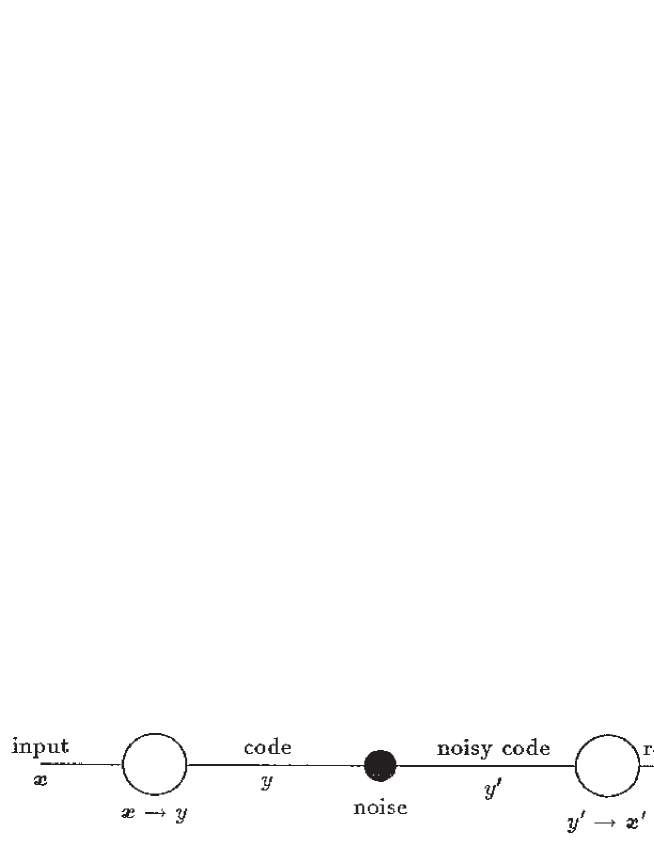
Figure 18: Encoding and decoding in a noisy vector quantiser.

We may represent the encoding and decoding operations together with the noise process diagrammatically as shown in Figure 18, which is a trivially modified version of Figure 17. By functionally differentiating $D_{2}$ with respect to $y(x)$ and $x^{\prime}(y)$ we obtain

$$\frac{\delta D_{2}}{\delta y(x)} \left.=P(x)\int dn\pi(n)\frac{\partial}{\partial y}\left\|x^{\prime}(y)-x\right\|^{2}\right|_{y=y(x)+n}$$ (45)

$$\frac{\delta D_{2}}{\delta x^{\prime}(y)} =2\int dxP(x)\pi(y-y(x))\left(x^{\prime}(y)-x\right)$$ (46)

Equation 45 is a “smeared” version of Equation 39, so $\frac{\delta D_{2}}{\delta y(x)}=0$ does not lead to nearest neighbour encoding because the distances to other code vectors have to be taken into account in order to minimise the damaging effect of the noise process. However, it is usually a good approximation to use the nearest neighbour encoding scheme shown in Equation 41. Setting $\frac{\delta D_{2}}{\delta x^{\prime}(y)}=0$ in Equation 46 yields the optimum decoding function

$$x^{\prime}(y)=\frac{\int dxP(x)\pi(y-y(x))x}{\int dxP(x)\pi(y-y(x))}$$ (47)

which should be compared with Equation 42. Alternatively, we may obtain a steepest descent scheme in the form

$$\begin{array}[]{cc}\delta x^{\prime}(y)=\epsilon\pi(y-y(x))\left(x-x^{\prime}(y)\right)&\operatorname{where}0<\epsilon<1\end{array}$$ (48)

which should be compared with Equation 43.

As in Section A.1, iterative optimisation schemes can be constructed in which we alternate the optimisation of the coding and decoding functions. Alternating Equation 41 (which approximately solves $\frac{\delta D_{2}}{\delta x^{\prime}(y)}=0$) and Equation 48 yields the standard topographic mapping training algorithm [9], which is widely used in various forms in neural network simulations.

A.3 Hierarchical vector quantisation

In Figure 19 we show the simplest type of hierarchical vector quantiser. It consists of an inner quantiser contained in the dashed box, surrounded by a pair of outer quantisers.

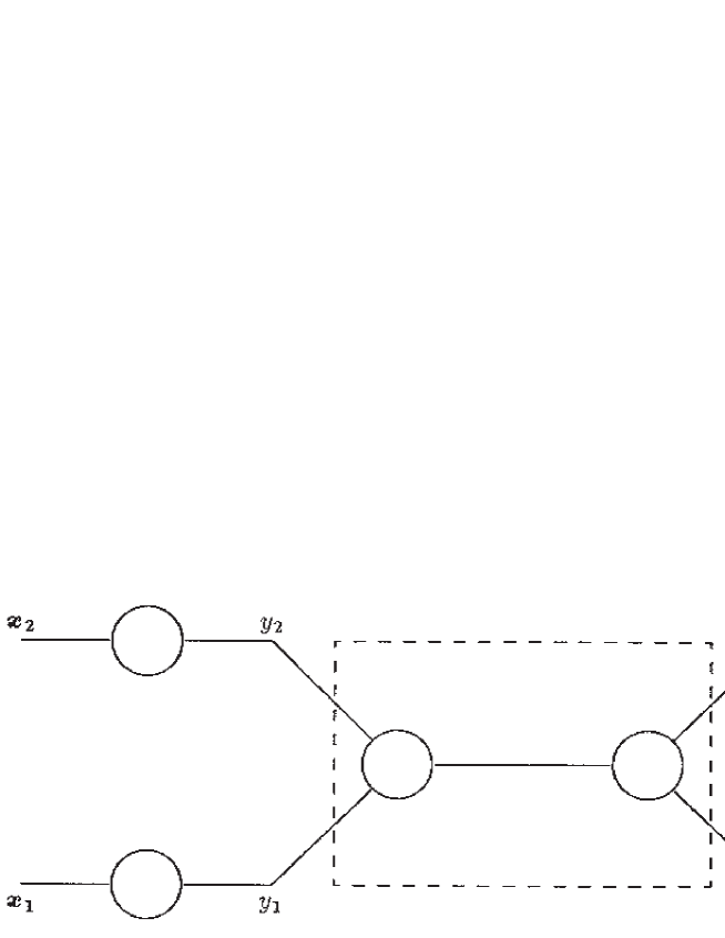
Figure 19: Encoding and decoding in a hierarchical vector quantiser.

If the part of the diagram contained in the dashed box were removed and direct connections made so that $y_{1}^{\prime}=y_{1}$ and $y_{2}^{\prime}=y_{2}$, then Figure 19 would reduce to a pair of independent vector quantisers of the type shown in Figure 17. The dashed box contains a vector quantiser which encodes $(y_{1},y_{2})$ to produce a code which it subsequently decodes to obtain $(y_{1}^{\prime},y_{2}^{\prime})$.

From the point of view of $y_{1}$ the effect of being passed through the inner quantiser is to modify $y_{1}$ thus $y_{1}\longrightarrow y_{1}^{\prime}$. A similar argument applies to $y_{2}\longrightarrow y_{2}^{\prime}$. The actual distortions $y_{1}^{\prime}-y_{1}$ and $y_{2}^{\prime}-y_{2}$ will be correlated in practice, but we shall model them as if they were independent processes, and thus reduce Figure 19 to two independent vector quantisers of the type shown in Figure 18.

This procedure can be extended to a hierarchical vector quantiser with any number of levels of nesting. From the point of view of the quantisers at any level, we shall model the effect of the quantisers inwards from that level as independent distortion processes. It turns out not to be critically important what precise distortion model one uses, provided that it approximately represents the overall scale of the distortion due to quantisation.

In [13] we presented in detail a phenomenological distortion model that we used to obtain an efficient training procedure for topographic mappings and their application to hierarchical vector quantisers. Alternatively, the standard topographic mapping training procedure in [9] could be used, but this is a rather inefficient algorithm. The basic training procedure may be obtained from Equation 48 as

1. Select a training vector $x$ at random from the training set.

2. Encode $x$ to produce $y$ ($=y(x)$).

3. For all $y^{\prime}$ do the following:

   1. Determine the corresponding code vector $x^{\prime}(y^{\prime})$.

   2. Move the code vector  $x^{\prime}(y^{\prime})$ directly towards the input vector $x$ by a distance $\epsilon\pi(y-y(x))|x-x^{\prime}(y)|$.

4. Go to step 1.

This cycle is repeated as often as is required to ensure convergence of the codebook of code vectors.

The standard method [9] specifies that $\pi(y^{\prime}-y)$ should be an even unimodal function whose width should be gradually decreased as training progresses. This allows coarse-grained organisation of the codebook to occur, followed progressively by ever more fine-grained organisation, until finally the algorithm converges towards an optimum codebook.

In our own modification [13] of the standard method we replace a shrinking $\pi(y^{\prime}-y)$ function acting on a fixed number of code vectors by a fixed $\pi(y^{\prime}-y)$ function acting on an increasing number of code vectors. There are many minor variations on this theme, but we find that it is sufficient to define

$$\pi(y^{\prime}-y)=\left\{\begin{array}[]{ccc}\epsilon&&y^{\prime}=y\\ \epsilon^{\prime}&&\left|y^{\prime}-y\right|=1\\ 0&&\left|y^{\prime}-y\right|>1\end{array}\right.$$ (49)

where we have absorbed $\epsilon$ in Equation 48 into the definition of $\pi(y^{\prime}-y)$. We use a binary sequence of codebook sizes $N=2,4,8,16,32,\cdots$, where each codebook is initialised by interpolation from the next smaller codebook. We find that the following parameter values yield adequate convergence: $\epsilon=0.1$, $\epsilon^{\prime}=0.05$, and we perform $20N$ training updates before doubling the value of $N$ and progressing to the next larger size of codebook. The $N=2$ codebook can be initialised using a random pair of vectors from the training set.

Appendix B Relationship to WISARD

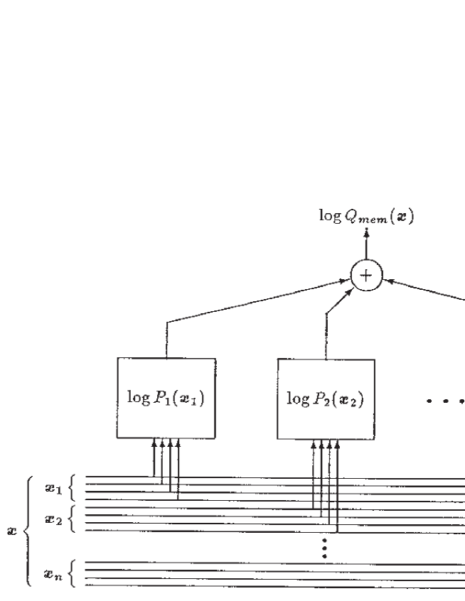
Figure 20: Single layer ACE is WISARD.

The second bracketed term in Equation 24 could be implemented in hardware as shown in Figure 20. This implementation assumes that the state vector $x$ is quantised by representing each of its components using a finite number of binary digits (bits). Note that we have taken advantage of the fact that we are discussing a single layer network in order to simplify the notation in Figure 20 (as compared with Equation 24). The $i$-th block in this circuit is a random access memory (RAM) which records a transformation from $x_{i}$ (the address of an entry in the RAM) to $\log P_{i}(x_{i})$ (the corresponding entry in the RAM). The data bus at the bottom of Figure 20 carries the components of $x$ (represented bitwise) to the relevant RAM. Note that each bit of $x$ is used exactly once in forming addresses for the RAM, so the mapping from $x$ to the set of addresses is bijective. The upper part of Figure 20 shows how the outputs are directed to an accumulator where they are summed to form $\log Q_{\textup{mem}}(x)$.

Figure 20 is a variant of the WISARD pattern recognition network [15]. The elements that our MEM solution and WISARD have in common are: a bijective mapping from the bits of an input state vector onto the address lines of a set of RAMs, and the accumulation of the outputs of the RAMs to form the overall network output.

However, there are some differences between the single layer ACE and the WISARD prescriptions for the contents of the RAMs. ACE specifies a set of functions (i.e. logarithms of marginal probabilities) to tabulate in the RAMs. Suppose that we truncate these table entries to a 1-bit representation, so that we use 0 to represent small logarithmic probabilities and 1 to represent large logarithmic probabilities. Each entry (i.e. 1 or 0) in the table then records whether the configuration of binary digits (i.e. the address of the entry) frequently occurs in the set of patterns corresponding to $P(x)$ (the “training set”). The final output is therefore the total number of 1’s that the input pattern addresses in the $n$ tables. In effect, this is the total number of coincidences between configurations of bits in the input pattern and those in a predefined category. This 1-bit version of ACE is qualitatively the same as the table look-up and summation operations performed in the simplest WISARD network, which completes the connection that we sought between ACE and WISARD.

References

- [1] Luttrell, S. P. (1987). Markov random fields: a strategy for clutter modelling. In Proc. AGARD Conf. on Scattering and Propagation in Random Media (pp. 7.1–7.8).
- [2] Luttrell, S. P. (1987). The use of Markov random field models in sampling scheme design. In Proc. SPIE Int. Symp. on Inverse Problems in Optics (pp. 182–188). New York: SPIE.
- [3] Luttrell, S. P. (1987). Designing Markov random field structures for clutter modelling. In Radar 87 (pp. 222–226). London: IEE.
- [4] Luttrell, S. P. (1987). The use of Markov random field models to derive sampling schemes for inverse texture problems. Inverse Problems, 3(2), 289–300.
- [5] Luttrell, S. P. (1988). A maximum entropy approach to sampling function design. Inverse Probl., 4(3), 829–841.
- [6] Ackley, D. H., Hinton, G. E., & Sejnowski, T. J. (1985). A learning algorithm for Boltzmann machines. Cognitive Sci., 9, 147–169.
- [7] Haralick, R. M., Shanmugam, K., & Dinstein, I. (1973). Textural features for image classification. IEEE Trans. Syst. Man Cyb., 3(6), 610–621.
- [8] Luttrell, S. P. (1989). The use of Bayesian and entropic methods in neural network theory. In G. Erickson, J. T. Rychert & C. R. Smith (Ed.), Maximum Entropy and Bayesian Methods (pp. 363–370). Dordtrecht: Kluwer.
- [9] Kohonen, T. (1984). Self-Organisation and Associative Memory. Berlin: Springer-Verlag.
- [10] Luttrell, S. P. (1988). Self organising multilayer topographic mappings. In Proc. IEEE Conf. on Neural Networks (pp. 93–100).
- [11] Luttrell, S. P. (1988). Image compression using a neural network. In Proc. IGARSS Conf. on Remote Sensing (pp. 1231–1238).
- [12] Luttrell, S. P. (1989). Self-organisation: a derivation from first principles of a class of learning algorithms. In Proc. IEEE Conf. on Neural Networks (pp. 495–498).
- [13] Luttrell, S. P. (1989). Hierarchical vector quantisation. Proc. Inst. Electr. Eng. I, 136(6), 405–413.
- [14] Luttrell, S. P. (1990). Derivation of a class of training algorithms. IEEE Trans. Neural Networ., 1(2), 229–232.
- [15] Aleksander, I., & Stonham, T. J. (1979). Guide to pattern recognition using random access memories. Comput. Digital Techniques, 2, 29–40.
- [16] Brodatz, P. (1966). Textures - A Photographic Album for Artists and Designers. New York: Dover.
- [17] Jaynes, E. T. (1968). Prior probabilities. IEEE Trans. Syst. Sci. Cyb., 4(3), 227–241.
- [18] Jaynes, E. T. (1982). On the rationale of maximum entropy methods. Proc. IEEE, 70(9), 939–952.
- [19] Luttrell, S. P. (1989). Hierarchical self-organising networks. In Proc. IEE Conf. on Artificial Neural Networks (pp. 2–6). London: IEE.
- [20] Luttrell, S. P. (1989). Image compression using a multilayer neural network. Patt. Recogn. Lett., 10(1), 1–7.
- [21] Linde, Y., Buzo, A., & Gray, R. M. (1980). An algorithm for vector quantiser design. IEEE Trans. Commun., 28(1), 84–95.
- [22] Kumazawa, H., Kasahara, M., & Namekawa, T. (1984). A construction of vector quantisers for noisy channels. Electron. Eng. Japan B, 67(4), 39–47.
- [23] Farvardin, N. (1990). A study of vector quantisation for noisy channels. IEEE Trans. Inform. Theory, 36(4), 799–809.