Finite-Length Scaling and Finite-Length Shift for Low-Density Parity-Check Codes

Abstract

Consider communication over the binary erasure channel ${\rm BEC}(\epsilon)$ using random low-density parity-check codes with finite-blocklength $n$ from ‘standard’ ensembles. We show that large error events is conveniently described within a scaling theory, and explain how to estimate heuristically their effect. Among other quantities, we consider the finite length threshold $\epsilon^{*}(n)$, defined by requiring a block error probability ${\rm P}_{\rm B}=1/2$. For ensembles with minimum variable degree larger than two, the following expression is argued to hold

$$\epsilon^{*}(n)=\epsilon^{*}-\epsilon^{*}_{1}\,n^{-2/3}+\Theta(n^{-1})\,,$$

with a calculable shift parameter $\epsilon^{*}_{1}>0$.

1 Introduction

Assessing the performances of finite-blocklength iterative coding systems is an important open issue in modern coding theory. A particular case of such a task consists in the study of low-density parity-check code (LDPC) ensembles, when used for communicating over the binary erasure channel ${\rm BEC}(\epsilon)$. A consistent effort has been devoted to this case, with the hope of a positive feedback on the general problem [4, 10, 11, 12, 14]. Some lessons can be drawn from the results obtained so far:

Approximate! While density evolution (DE) provides exact thresholds in the large blocklength limit, there is little hope to compute exact performances (bit or block error rates ${\rm P}_{\rm b}$ and ${\rm P}_{\rm B}$) at finite blocklength $n$. For the ${\rm BEC}(\epsilon)$, ${\rm P}_{\rm b}$ and ${\rm P}_{\rm B}$ are determined by a set of recursions [4] whose evaluation has complexity $\Theta(n^{\kappa})$. However the exponent $\kappa$ grows with the irregularity of the ensemble (more precisely, with the number of probabilistically inequivalent types of node in the Tanner graph). Given the large degree of irregularity necessary for approaching capacity, an exact calculation becomes prohibitive already for moderate blocklengths. The situation can unlikely be simpler for more general channel models.

It is therefore crucial to develop approximate estimates of finite-length performances.

Small error events. Consider, for the sake of simplicity, communication over ${\rm BEC}(\epsilon)$ using an LDPC ensemble. Below the threshold $\epsilon^{*}$ for iterative decoding, the typical size of error events (the number of erased bits after decoding) is of order $1$. Above threshold, the same size is of order $n$ (the bit error probability is finite). One can regard the failure of iterative decoding at $\epsilon^{*}$ as due to the divergence (on the $\Theta(1)$ scale) of the size of typical error events.

The probability of small error events is readily evaluated through the union bound. For a code with minimum variable degree $l_{\rm min}$, the expected number of error events involving $E$ bits is $\Theta(n^{E-\lceil El_{\rm min}/2\rceil}\epsilon^{E})$, as long as $E$ is kept finite in the $n\to\infty$ limit. If $l_{\rm min}>2$, this quantity decreases by a factor $n$ (or more) each time $E$ increases by one. This suggests that only very small error events have a non-negligible probability: their contribution can be computed exactly [10] and compares favorably with recursive calculations or numerical simulations. Moreover, in the vast majority of elements from the ensemble, such error events are strictly absent.

If $l_{\rm min}=2$, the dominating error events involve uniquely degree 2 variable nodes, and have the topology of cycles in the Tanner graph. The number of such structures is $\Theta(n^{2E})$: one can chose both the variables and the check nodes involved. Their probability is $\Theta(\Lambda_{2}^{E}\epsilon^{E}n^{-2E})$, where we denoted by $\Lambda_{l}$ the fraction of variable nodes having degree $l$. In fact: the variables must be erased (which explains the factor $\epsilon^{E}$); they must have degree 2 (factor $\Lambda_{2}^{E}$); and they must be connected to the previously chosen check nodes (factor $n^{-2E}$). Unlike in the case $l_{\rm min}>2$, the resulting typical size depends upon $\epsilon$. Detailed calculations can be carried on for cycle ensembles: one finds $E_{\rm typ}\sim|\epsilon^{*}-\epsilon|^{-1}$ as $\epsilon\uparrow\epsilon^{*}$. The divergence of error events size ‘drives’ the failure of iterative decoding above $\epsilon^{*}$.

Large error events. Computing the probability of small (i.e. finite in the $n\to\infty$ limit) error events is a conceptually straightforward task. While in the case $l_{\rm min}>2$ one has do the computation for just a few small structures, if degree-two nodes are present, an infinite number of contributions must be summed over. In both cases, this approach yields a simple and accurate description of the error probability in the noise regime for which ${\rm P}_{\rm b}=\Theta(n^{1-\lceil l_{\rm min}/2\rceil})$. This is the so-called error-floor region.

What about the waterfall region? The description in terms of finite-size error events cannot account for this regime. Take for instance the case $l_{\rm min}>2$. As long as the error size $E$ is finite, its probability decreases rapidly with $E$. The breakdown of iterative decoding at $\epsilon^{*}$ can therefore be ascribed uniquely to error events whose size diverges with $n$. Analogously, for cycle ensembles the typical size of finite error events diverges at $\epsilon^{*}$. This conclusion can be extended to general irregular ensembles: in order to describe the waterfall region, large error events have to be taken into account.

This remark implies several theoretical problems. First of all, no enumeration of all the configurations (by this we mean stopping sets in the ${\rm BEC}(\epsilon)$ case, and any suitable generalization for other channels) responsible for errors is possible in the waterfall regime. In fact, it is likely that the number of relevant ‘topologies’ diverges with the blocklength. Second, we cannot think of the set of wrongly decoded bits as the union of several small ‘error events’, which are probabilistically independent. In more practical terms: the union bound is not a reliable tool in this regime.

Yet, as optimized ensembles approach capacity, controlling the waterfall region is of utmost interest. We developed an approach to this problem for the ${\rm BEC}(\epsilon)$ case, which yields extremely satisfactory results. The methods are complementary to the stopping-sets analysis and build upon the description of iterative decoding by Luby et al. [8, 7]. Although the extension to general channel models is likely to require a considerable effort, one can learn a general lesson about which kind of characterization can be hoped for in the waterfall regime.

Consider, for the sake of simplicity the case of $l_{\rm min}>2$. We find that there exists a non-negative constant $\nu$ and some non-negative function $f(z)$ so that

$$\lim_{n\rightarrow\infty}{\mbox{\rm P}}_{\rm B}(n,\epsilon_{n})=f(z)\,,$$ (1)

where the $n\to\infty$ limit is taken by keeping $n^{\frac{1}{\nu}}(\epsilon^{*}-\epsilon_{n})=z$ fixed. In other words, if one plots ${\mbox{\rm P}}_{\rm B}(n,\epsilon)$ as a function of $z=n^{\frac{1}{\nu}}(\epsilon^{*}-\epsilon)$ then, for increasing $n$ these finite-length curves are expected to converge to some function $f(z)$. The function $f(z)$ decreases smoothly from $1$ to $0$ as its argument changes from $-\infty$ to $+\infty$. This means that all finite-length curves are, to first order, scaled versions of some mother curve $f(z)$. It might be helpful to think of the threshold $\epsilon^{*}$ as the zero order term in a Taylor series. Then the above scaling, if correct, represents the first order term. In fact, one can even refine the analysis to include higher order terms and write

$${\mbox{\rm P}}_{\rm B}(n,\epsilon) = f(z)+n^{-\omega}g(z)+o(n^{-\omega}),$$ (2)

where $\omega$ is some positive real number and $g(z)$ is the second order correction term.

For ensembles with $l_{\rm min}=2$ (and in particular, for ensembles whose threshold is fixed by the local stability condition) Eq. (1) must be properly generalized. We refer to Ref. [3] for an example.

Figure 1: Scaling of ${\mbox{\rm P}}_{\rm B}(n,\sigma)$ for transmission over BAWGNC$(\sigma)$ and a quantized version of belief propagation decoding implemented in hardware. The threshold for this combination is $\left(E_{b}/N_{0}\right)^{*}_{\text{dB}}\approx 1.19658$. The blocklengths $n$ are $n=1000$, $2000$, $4000$, $8000$, $16000$ and $32000$, respectively. The solid curves represent the simulated ensemble averages. The dashed curves are computed according to the refined scaling law (10) with scaling parameters $\alpha=0.8694$ and $\beta=5.884$. These parameters were fitted to the empirical data.

It is worth making a couple of remarks. First of all, the form (1), wherever it can be argued to hold, allows a precise definition of what is meant by “waterfall” region. This is going to be the interval of channel parameters $\epsilon^{*}-C_{-}n^{-\frac{1}{\nu}}\leq\epsilon\leq\epsilon^{*}+C_{+}n^{-\frac{1}{\nu}}$ for some positive constants $C_{-}$ and $C_{+}$. Second, even in cases in which the function $f(z)$ cannot be determined analytically, the statement (1) is highly informative, since it reduces a two-variable function to a single-variable one. Moreover, in several cases, $f(z)$ can be efficiently given in terms of a few parameters. This opens the way to empirical applications of Eq. (1). An example is provided in Fig. (1).

Finite-length optimization of code ensembles is an issue of great practical relevance. We think that the scaling description (1)-(2) may be an important step towards a mathematically well-founded solution of this task.

A first numerical investigation of finite-size scaling for LDPC codes was presented in Ref. [9]. Earlier accounts of the present work appeared in [1, 2], and a complete version in [3]. Related ideas were put forward by Lee and Blahut [6] and Zemor and Cohen [13].

2 Heuristic arguments

In this paper we consider standard LDPC$(n,\lambda,\rho)$ ensembles. Here $n$ is the blocklength, and $\lambda$ and $\rho$ denote the degree distribution of (respectively) variable and check nodes from an edge perspective. For the sake of simplicity, we shall often refer to regular ensembles with left degree $l$, and right degree $k$. The corresponding degree distributions read $\lambda(x)=x^{l}$ and $\rho(x)=x^{k}$.

In order to analyze the iterative decoder, we adopt the point of view introduced by Luby et al. in [8, 7]. According to this description, the algorithm proceeds as follows (we assume the all-zeros codeword to be transmitted and describe the action of the algorithm on the Tanner graph). Given the received message, the decoder deletes all received variable nodes and their incident edges. In this way one arrives at a residual graph. The decoder proceeds now in an iterative fashion. If the residual graph contains no degree-one check nodes the decoding process stops. Otherwise, the decoder randomly chooses one such degree-one check node and deletes it together with the corresponding variable node and all its incident edges. In this way a new residual graph results and a new iteration starts. Decoding is successful if all the graph gets deleted by this procedure. In the opposite case, the decoder gets stucked in a stopping set.

The state of the algorithm after a fixed number of iterations can be entirely described by a finite set of integers, providing the number of variable and check nodes of a given degree. Let us denote this vector of integers by $\underline{x}$. For regular ensembles the situation is even simpler: it is enough to specify the total number of variable nodes $v$, the number of degree-one check nodes $s$, and the number of check nodes of higher degree $t$. Therefore, in this case $\underline{x}=(v,s,t)$. Notice that, when decoding starts, these variables are of order $\Theta(n)$. Each iteration of the decoding procedure described above, amounts to a finite increment (or decrement) in these variables. In particular, for the regular case: $v$ decreases by one; $s$ decreases by one (the check node chosen at that iteration) and increases by the number of degree-two check nodes which are neighbors of the newly deleted variable; $t$ decreases by this last quantity. It is easy to realize that the probability distribution of these increments (decrements) depends upon $v,s,t$ only on the scale $n$. More precisely the probability of a variation $(\Delta v,\Delta s,\Delta t)$ is (up to $1/n$ corrections) a smooth function of $v/n$, $s/n$, and $t/n$.

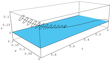
Figure 2: A pictorial representation of density and covariance evolution for the LDPC($n,x^{2},x^{5})$ ensemble. Notice that the ellipsoids corresponding to $(s,t)$ covariances should be regarded as living on a smaller (by a factor $\sqrt{n}$) scale than the typical trajectory.

Call $\underline{x}(\ell)$ the state after $\ell$ iterations, and consider the change in state $\delta\underline{x}=\underline{x}(\ell+\delta\ell)-\underline{x}(\ell)$ in a time $\delta\ell$. If $\delta\ell$ is much smaller than $\Theta(n)$, then also $|\delta\underline{x}|\ll n$. Therefore each step in the interval $[\ell,\ell+\delta\ell]$ is independent and identically distributed. If $\delta\ell$ is nevertheless much larger than 1, we can apply the central limit theorem to deduce that $\delta\underline{x}$ is, with good approximation, a multi-dimensional gaussian variable with mean of order $\delta\ell$ and standard deviation of order $\sqrt{\delta\ell}$. Since, for $\delta\ell\gg 1$, $\sqrt{\delta\ell}\ll\delta\ell$, one can, to a first approximation neglect fluctuations. This was the essential step taken in [8, 7]. These authors showed that $\underline{x}(\ell)$ concentrates around its average value $\underline{x}_{\rm av}(\ell)\approx n\underline{z}(\ell/n)$, with $\underline{z}(\tau)$ solution of the a set of ordinary differential equations:

$$\frac{dz_{i}}{d\tau}=f_{i}(\underline{z},\tau)\,.$$ (3)

These are nothing but the density evolution equations. They are integrated with an initial condition depending upon the erasure probability.

A typical decoding trajectory is reported in Fig. 2. For $\epsilon<\epsilon^{*}$, it reaches the $(v=0,s=0,t=0)$ point before touching the $s=0$ plane: decoding is successful. For $\epsilon>\epsilon^{*}$, it touches the $s=0$ plane before the $(v=0,s=0,t=0)$ point: a stopping set has been reached.

Once the typical trajectory is found, one can compute distribution of $\underline{x}(\ell)-\underline{x}_{\rm av}(\ell)$. The procedure is conceptually simple. Consider $\ell\approx n\tau$ for some fixed $\tau$ and decompose the interval $[0,\ell]$ into sub-intervals of size $\delta\ell$, with $1\ll\delta\ell\ll n$. Within each sub-interval we can apply the argument outlined above to show that $\delta\underline{x}$ is gaussian with standard deviation of order $\sqrt{\delta\ell}$. Gluing together $n/\delta\ell$ such intervals we deduce that $\underline{x}(\ell)-\underline{x}_{\rm av}(\ell)$ is gaussian with standard deviation of order $\sqrt{n}$. This has immediate implications for the decoding performances. In fact, as soon as the average trajectory passes within a distance of order $\sqrt{n}$ above the $s=0$ plane, fluctuations will produce a finite probability of hitting the plane. Vice-versa, if the average trajectory passes $\sqrt{n}$ below the $s=0$ plane, decoding can nevertheless be successful with finite probability. Recall that the erasure probability sets the initial condition. It is easy to realize that a change $\delta\epsilon$ in the channel parameter implies a change of order $n\,\delta\epsilon$ in the average trajectory $\underline{x}_{\rm av}(\ell)$. At threshold ($\epsilon=\epsilon^{*}$), $\underline{x}(\ell)$ is just tangent to the $s=0$ plane. This implies that the failure probability is strictly between $0$ and $1$ as long as $n|\epsilon-\epsilon^{*}|\lesssim\sqrt{n}$. This suggest that the scaling form (1) holds with $\nu=2$.

The above argument can be made both quantitative and rigorous: the procedure for computing gaussian fluctuations around the typical trajectory has been named covariance evolution [3] and it is not much harder than usual density evolution. We refer to the next section for a more precise account of the results. Unhappily, when compared with detailed simulations, or with exact computations obtained from recursion relations, the results are not very accurate. The reason lies in some subtle effect that produces sizeable corrections of the form (2). It turns out that $\omega=1/6$: this implies large corrections even for quite large blocklengths ($n$ in the range $10^{3}\div 10^{5}$). Since it turns out that $g(z)\propto f^{\prime}(z)$, the same corrections can be attributed to a finite-length shift of the iterative threshold:

$$\epsilon^{*}(n)=\epsilon^{*}-\epsilon^{*}_{1}\,n^{-2/3}+\Theta(n^{-1})\,,$$ (4)

with a positive (ensemble-dependent) constant $\epsilon^{*}_{1}$.

Figure 3: A pictorial view of decoding trajectories near the critical point. The type of trajectory depicted here is responsible for the finite-length shift of the iterative threshold (4).

It is not hard to understand the origin of the shift (4) heuristically. In a nutshell: when passing $\sqrt{n}$ above the $s=0$ plane, the decoding trajectory has many occasions to fail. At any time, a fluctuation may imply it touching the plane. On the other hand, for decoding to be successful, all fluctuations must be lucky enough to keep the trajectory away from the plane. This asymmetry leads to a finite-size lowering of the threshold.

In order to understand the $-2/3$ exponent in Eq. (4), it may be convenient to consider a toy example, cf. Fig. 3. Here the state is describe by a single integer $x$, playing the role of $s$ in the decoding problem, evolving over discrete time $\ell$. Both $x$ and $\ell$ are typically of order $n$, and the increment probabilities of $x$ depends smoothly on $x/n$ and $\ell/n$. Finally, the average trajectory $x_{\rm av}(\ell)$ has a minimum at $\ell_{*}$, with $x_{\rm av}(\ell_{*})=0$, and

$$x_{\rm av}(\ell)=\frac{1}{2n}(\ell-\ell_{*})^{2}+\Theta((\ell-\ell_{*})^{3}/n^{2})\,,$$ (5)

near the minimum. In other words the minimum is ‘non-degenerate’. This is the situation for iterative decoding at $\epsilon=\epsilon^{*}$ under mild conditions on the code ensemble. We want to compute the ‘failure’ probability, ${\mbox{\rm P}}(n)$ i.e. the probability for the trajectory to touch the $x=0$ plane, which corresponds to the block error probability in the decoding problem.

Within a first approximation $x(\ell)$ is at any time a gaussian variable with mean $x_{\rm av}(\ell)$ and standard deviation of order $\sqrt{n}$. The failure probability can be estimated as the probability for $x(\ell=\ell_{*})\leq 0$. Since $x_{\rm av}(\ell=\ell_{*})=0$, we get ${\mbox{\rm P}}(n)=1/2$. The crucial point is now that, even if $x(\ell_{*})>0$, the trajectory has some probability for touching the $x=0$ plane either for $\ell<\ell_{*}$ or for $\ell>\ell_{*}$. What matters is clearly the location of the minimum $\ell_{g}$. The trajectory does not touch the $x=0$ plane if and only if $x(\ell_{g})>0$.

Let us now try to estimate the position of the minimum $\ell_{g}$. This is the outcome of a balance between two competing forces. On the one hand, the average trajectory is bent upward and forces $\ell_{g}$ to be close to $\ell_{*}$. This yields a contribution to $x(\ell)-x(\ell_{*})$ which is of order $(\ell-\ell_{*})^{2}/2n$. On the other hand, by moving away from $\ell_{*}$ one can take advantage of fluctuations, $[x(\ell)-x(\ell_{*})]-[x_{\rm av}(\ell)-x_{\rm av}(\ell_{*})]$ which are typically of order $\sqrt{\ell-\ell_{*}}$. The location of $\ell_{g}$ is estimated by balancing these two effects: $(\ell-\ell_{*})^{2}/2n\sim\sqrt{\ell-\ell_{*}}$. We get therefore

$$|\ell_{g}-\ell_{*}|=O(n^{2/3})\,,\;\;\;\;\;|x(\ell_{g})-x(\ell_{*})|=O(n^{1/3})\,.$$ (6)

The above argument implies that the failure probability is slightly larger than $1/2$. One can in fact fail either if $x(\ell_{*})<0$ (and this happens with probability $1/2$), or if $x(\ell_{*})=O(n^{1/3})$ because, in this case, $x(\ell_{g})$ can be $O(n^{1/3})$ below $x(\ell_{*})$. What is the probability of $x(\ell_{*})=O(n^{1/3})$? We know that $x(\ell_{*})$ is, with good approximation a gaussian variable with mean $0$ and standard deviation $\Theta(\sqrt{n})$. Therefore the probability is of order $n^{-1/2}\cdot n^{1/3}=n^{-1/6}$. We find therefore the estimate

$${\mbox{\rm P}}(n)=\frac{1}{2}+{\mbox{\rm P}}_{1}\,n^{-1/6}+\dots\,.$$ (7)

Remarkably, the constant ${\mbox{\rm P}}_{1}$ can be calculated exactly [3] and depends uniquely upon the transition probabilities near $x(\ell_{*})$. Once the axes $x$ and $\ell$ have been properly scaled ${\mbox{\rm P}}_{1}$ is given by an integral expression in terms of Airy functions.

When adapted to the coding problem, the above argument yields $\omega=1/6$ in Eq. (2). If we define the finite-size threshold $\epsilon^{*}(n)$ by ${\rm P}_{\rm B}(n,\epsilon^{*}(n))=1/2$, we get Eq. (4).

3 Results

The heuristic arguments presented in the previous Section can be put on precise quantitative bases. For some of them we were able to provide a rigorous foundation, leading to the following:

Lemma 1

[Scaling of Unconditionally Stable Ensembles] Consider transmission over the BEC$(\epsilon)$ using random elements from an ensemble $\rm{LDPC}(n,\lambda,\rho)$ which has a single critical point and is unconditionally stable. Let $\epsilon^{*}=\epsilon^{*}(\lambda,\rho)$ denote the threshold and let $\nu^{*}$ denote the fractional size of the residual graph at the critical point corresponding to the threshold. Fix $z$ to be $z:=\sqrt{n}(\epsilon^{*}-\epsilon)$. Let ${\mbox{\rm P}}_{\rm{b}}(n,\lambda,\rho,\epsilon)$ denote the expected bit erasure probability and let ${\mbox{\rm P}}_{\rm{B},\gamma}(n,\lambda,\rho,\epsilon)$ denote the expected block erasure probability due to errors of size at least $\gamma\nu^{*}$, where $\gamma\in(0,1)$. Then as $n$ tends to infinity,

$${\mbox{\rm P}}_{\rm{B},\gamma}(n,\lambda,\rho,\epsilon) = Q\left(\frac{z}{\alpha}\right)(1+o_{n}(1)),$$ (8)

$${\mbox{\rm P}}_{\rm{b}}(n,\lambda,\rho,\epsilon) = \nu^{*}Q\left(\frac{z}{\alpha}\right)(1+o_{n}(1)),$$ (9)

where $\alpha=\alpha(\lambda,\rho)$ is a constant which depends on the ensemble.

Unhappily, we were not able to derive powerful enough estimate for making the ‘shift’ argument rigorous. However, the difficulty is more technical than conceptual. We formulate therefore the following:

Conjecture 1

[Refined Scaling of Unconditionally Stable Ensembles] Consider transmission over the BEC$(\epsilon)$ using random elements from an ensemble $\rm{LDPC}(n,\lambda,\rho)$ which has a single critical point and is unconditionally stable. Let $\epsilon^{*}=\epsilon^{*}(\lambda,\rho)$ denote the threshold and let $\nu^{*}$ denote the fractional size of the residual graph at the threshold. Let ${\mbox{\rm P}}_{\rm{b}}(n,\lambda,\rho,\epsilon)$ denote the expected bit erasure probability and let ${\mbox{\rm P}}_{\rm{B},\gamma}(n,\lambda,\rho,\epsilon)$ denote the expected block erasure probability due to errors of size at least $\gamma\nu^{*}$, where $\gamma\in(0,1)$. Fix $z$ to be $z:=\sqrt{n}(\epsilon^{*}-\beta n^{-\frac{2}{3}}-\epsilon)$. Then as $n$ tends to infinity,

$${\mbox{\rm P}}_{\rm{B},\gamma}(n,\lambda,\rho,\epsilon) = Q\left(\frac{z}{\alpha}\right)\left(1+O(n^{-1/3})\right),$$ (10)

$${\mbox{\rm P}}_{\rm{b}}(n,\lambda,\rho,\epsilon) = \nu^{*}Q\left(\frac{z}{\alpha}\right)\left(1+O(n^{-1/3})\right),$$ (11)

where $\alpha=\alpha(\lambda,\rho)$ and $\beta=\beta(\lambda,\rho)$ are constants which depend on the ensemble.

In Table 1 we report the values of the scaling parameters for a few regular ensembles. These parameters are obtained by integrating a set of ordinary differential (covariance evolution) equations and are easily pushed to great precision.

$l$	$k$	$\epsilon^{*}$	$\alpha$	$\beta/\Omega$
3	4	$0.6473$	$0.260115$	$0.593632$
3	5	$0.5176$	$0.263814$	$0.616196$
3	6	$0.4294$	$0.249869$	$0.616949$
4	5	$0.6001$	$0.241125$	$0.571617$
4	6	$0.5061$	$0.246776$	$0.574356$
5	6	$0.5510$	$0.228362$	$0.559688$
6	7	$0.5079$	$0.280781$	$0.547797$
6	12	$0.3075$	$0.170218$	$0.506326$

Table 1: Thresholds and scaling parameters for some regular standard ensembles $\lambda(x)=x^{l}$, $\rho(x)=x^{k}$. The shift parameter is given as $\beta/\Omega$ where $\Omega$ is the universal constant defined in Ref. [3] in terms of Airy functions, and whose numerical value is very close to 1.

Finally, in Fig. 4 we compare the refined scaling form provided by Conjecture 1, with the exact error probability computed by recursion. The agreement is excellent.

Figure 4: Scaling of ${\mbox{\rm P}}_{\rm B}(n,\epsilon)$ for transmission over BEC$(\epsilon)$ and belief propagation decoding. The threshold for this combination is $\epsilon^{*}\approx 0.42944$, see Table 1. The blocklengths/expurgation parameters are $n/s=1024/24$, $2048/43$, $4096/82$ and $8192/147$, respectively. (More precisely, we assume that the ensembles have been expurgated so that graphs in this ensemble do not contain stopping sets of size $s$ or smaller.) The solid curves represent the exact ensemble averages. The dashed curves are computed according to the refined scaling law stated in Conjecture 1 with scaling parameters $\alpha=\sqrt{0.249869^{2}+\epsilon^{*}(1-\epsilon^{*})}$ and $\beta=0.616045$, see Table 1.

References

- [1] A. Amraoui, A. Montanari, T. Richardson, and R. Urbanke, Finite-length scaling for iteratively decoded LDPC ensembles, in Proc. 41th Annual Allerton Conference on Communication, Control and Computing, Monticello, IL, 2003.
- [2] , Finite-length scaling for iteratively decoded LDPC ensembles, in Proc. IEEE International Symposium on Information Theory, Chicago, Illinois, June-July 2004, 2004.
- [3] , Finite-length scaling for iteratively decoded LDPC ensembles, submitted to IEEE Transactions on Information Theory.
- [4] C. Di, D. Proietti, T. Richardson, E. Telatar, and R. Urbanke, Finite length analysis of low-density parity-check codes on the binary erasure channel, IEEE Trans. Inform. Theory, 48 (2002), pp. 1570–1579.
- [5] M. E. Fisher, in Critical Phenomena, International School of Physics Enrico Fermi, Course LI, edited by M. S. Green, (Academic, New York, 1971).
- [6] J. Lee and R. Blahut, Bit error rate estimate of finite length turbo codes, in Proceedings of ICC’03, Anchorage Alaska, USA, May 11–15 2003, p. 2728.
- [7] M. Luby, M. Mitzenmacher, A. Shokrollahi, and D. Spielman, Efficient erasure correcting codes, IEEE Trans. Inform. Theory, 47 (2001), pp. 569–584.
- [8] M. Luby, M. Mitzenmacher, A. Shokrollahi, D. Spielman, and V. Stemann, Practical loss-resilient codes, in Proceedings of the th annual ACM Symposium on Theory of Computing, 1997, pp. 150–159.
- [9] A. Montanari, Finite-size scaling of good codes, in Proc. 39th Annual Allerton Conference on Communication, Control and Computing, Monticello, IL, 2001.
- [10] T. Richardson, A. Shokrollahi, and R. Urbanke, Error-floor analysis of various low-density parity-check ensembles for the binary erasure channel. To be presented at ISIT’02 in Lausanne, 2002.
- [11] , Finite-length analysis of various low-density parity-check ensembles for the binary erasure channel, in IEEE International Symposium on Information Theory, Lausanne, Switzerland, June 30–July 5 2002, p. 1.
- [12] T. Richardson and R. Urbanke, Finite-length density evolution and the distribution of the number of iterations for the binary erasure channel. in preparation, 2003.
- [13] G. Zemor and G. Cohen, The threshold probability of a code, IEEE Trans. Inform. Theory, 41 (1995), pp. 469–477.
- [14] J. Zhang and A. Orlitsky, Finite-length analysis of LDPC codes with large left degrees, in IEEE International Symposium on Information Theory, Lausanne, Switzerland, June 30–July 5 2002, p. 3.