Optimal Free-Space Management and Routing-Conscious Dynamic Placement for Reconfigurable Devices

Abstract

We describe algorithmic results on two crucial aspects of allocating resources on computational hardware devices with partial reconfigurability. By using methods from the field of computational geometry, we derive a method that allows correct maintainance of free and occupied space of a set of $n$ rectangular modules in time $O(n\log n)$; previous approaches needed a time of $O(n^{2})$ for correct results and $O(n)$ for heuristic results. We also show a matching lower bound of $\Omega(n\log n)$, so our approach is optimal. We also show that finding an optimal feasible communication-conscious placement (which minimizes the total weighted Manhattan distance between the new module and existing demand points) can be computed with $\Theta(n\log n)$. Both resulting algorithms are practically easy to implement and show convincing experimental behavior.

ACM Classification: C.3.e: Reconfigurable Hardware;
                                           F.2.2.c: Geometrical problems and computations

Keywords: Reconfigurable hardware, field-programmable gate array (FPGA), module placement, free space manager, routing-conscious placement, geometric optimization, line sweep technique, optimal running time, lower bounds.

1 Introduction

Reconfigurable Computing.

One of the cutting-edge aspects of modern reconfigurable computing is the possibility of partial reconfiguration of a device: A new module can be placed on a reconfigurable chip whithout interfering the computation of other modules. Clearly, this approach has advantages over a full reconfiguration of the whole chip. However, there is still a tremendous need for scientific progress: The technical possibilities for partial reconfiguration have been somewhat restricted, and manufacturers have been slow in providing possibilities, tools, and documentation. As a consequence, there has only been a limited amount of previous research on this topic.

New reconfigurable devices such as FPGAs offer increasing levels of partial reconfigurability, and chip sizes continue to grow. At the same time, static programming methodologies show an increasing use of pre-implementation by means of relocatable module libraries with bounding-box restrictions.

These developments place an ever-growing demand on the run-time management of resource allocation. As these tasks become more and more complex, one needs support in the form of operating systems [2] for managing both software and hardware processes (see Figure 1.)

\begin{picture}(8854.0,4498.0)(3139.0,-7598.0)\end{picture}

Figure 1: An operating system for reconfigurable computers.

Runtime space allocation, also known as temporal placement, is a central part in partially reconfigurable computing systems. In this paper, we present methods to solve two crucial issues for devices that allow for partial reconfiguration:

1. Given a set of $n$ rectangular modules that have been placed on a chip, identify all feasible positions for a new module.

2. Given a set of $n$ rectangular modules that have been placed on a chip, a new module, and demands for connecting it to existing sites, find a feasible position for the module that minimizes the total weighted distance to the given sites.

Related Work. The first of the above issues is the task of maintaining free space. Bazargan et al. [3] describe how to achieve this by maintaining the set of all maximal free rectangles; as this set can have size $\Omega(n^{2})$, the complexity is quadratic. Alternatively, they propose partitioning free space into only $O(n)$ free rectangles; the price for this improved complexity is the fact that no feasible placement may be found, even though one exists. Walder et al. [4] have suggested ways to reduce this deficiency and did report on experimental improvement, but their $O(n)$ procedure is still a heuristic approach that may fail in some scenarios. Thus, there remains a gap between $O(n^{2})$ methods that report an accurate answer, and $O(n)$ heuristics that may fail in some scenarios. Ahmadinia et al. [5] suggested maintaining occupied space instead of free space, but (depending on the computational model) their approach is still quadratic. Other current work on free-space management was presented by Tabero et al. [6, 7], who provide an $O(n^{2})$ approach based on keeping track of possible corner positions.

The above difficulty may have contributed to the fact that routing-conscious placement has received hardly any attention at all: Clearly, optimal placement of a new module has to go beyond feasible placement. In the context of configurable computing, this second aspect has only been treated very recently, in work by Ahmadinia et al. [5], who suggest a heuristic to find a feasible placement for a new module that has small total weighted Euclidean distance to a given set of demand points. In the area of discrete algorithms, two papers study a somewhat related problem: Karp et al. [8] consider the problem of arranging a set of records in a 2-dimensional array, such that the total weighted distance is minimized. In this context, all records have the same size (unit cells), and no previous records have been placed; on the other hand, all records have to be placed at once, which is different from our scenario. It should be noted that for the case of Manhattan distances, the resulting shape for large numbers of records can only be described by a differential equation, indicating surprising computational difficulties. In more recent work, Bender et al. [9] consider the problem of allocating $k$ processors in a grid supercomputer in the presence of occupied cells; this is a generalization of [8]. They also present empirical evidence that indeed the Manhattan distance between processors should be minimized for optimizing communication cost, and thus runtime of the resulting jobs. In this context, see also [10, 11, 12].

Our Results. We resolve both of the above issues:

• We give a $O(n\log n)$ method to provide a free-space manager (FSM). This approach uses a plane-sweep approach from computational geometry.

• We give a matching lower bound of $\Omega(n\log n)$ for locating a maximal free rectangle between a set of $n$ modules, showing that our method has optimal complexity.

• We show that our FSM can be extended to find a feasible position that minimizes total weighted Manhattan distance to existing sites. The resulting algorithm still has an optimal run time of $\Theta(n\log n)$.

• We describe implementation details to illustrate that our method is fast and easy.

• We provide experimental data to demonstrate the practical usefulness of our results.

The rest of this paper is organized as follows. In Section 2, we present our optimal FSM. Section 3 describes how to perform optimal routing-conscious placement. Section 4 shows implementation details and experimental data. The final Section 5 discusses possible implications and extensions of our work.

2 The Free-Space Manager

In this section we present our approach to free-space management. Our FSM is based on the observation that the occupied space consists of very simple geometric objects, namely $n$ placed rectangular modules. Put simply our free-space manager is a modification of the well-known algorithm ContourOfUnionOfRectangles (CUR) [13, 14, 15], for finding the contour of a union of axis-parallel rectangles. As the number of contour segments is linear in $n$, we achieve a running time of $O(n\log n)$. Note that we do not require the contour to be connected, i.e., our approach works even if there are holes in the arrangement.

2.1 Free-Space Manager Basics

Figure 2: A set of existing modules (white) on a rectangular chip and an additional module that has to be placed on the remaining free chip area (dark).

We consider an FPGA or other reconfigurable device and denote its width by $W$ and its height by $H$. Assumsing a coordinate origin in the lower left corner of the chip, we can describe the corresponding input by the quadruple $F=(0,0,W,H)$. On the device, a set $M=\{(x_{i},y_{i},w_{i},h_{i}):i\in\{1,2,\ldots,n\}\}$ of modules $m_{i}$ with widths $w_{i}$ and heights $h_{i}$ has been placed, with lower left corners at positions $(x_{i},y_{i})$. The task for the free-space manager is to identify regions where a new module $m$ with width $w_{m}$ and height $h_{m}$ can be placed.

Figure 3: Expanding existing modules and shrinking chip area and the new module reduces free-space management to managing free-space for a single point.

Figure 4: Resulting free space (dark).

As mentioned above, prior free-space managers maintained lists of unoccupied rectangles. Because the number of maximal empty rectangles is quadratic in the number of modules this clearly leads to quadratic running times. In [5], Ahmadinia et al. described how the management of free space can be simplified to finding a placement for a single point (see Figure 3) by transforming the problem data as follows: Shrink the area of the chip and simultaneously blow up the existing modules by half the width and half the height of the new module. This way the chip area is given by

$$F^{\prime} =(\frac{w_{m}}{2},\frac{h_{m}}{2},W-\frac{w_{m}}{2},H-\frac{h_{m}}{2})$$

and the set of placed modules $$M F^{\prime}$$ clipped by becomes

$$M^{\prime} =\{(x^{\prime}_{i},y^{\prime}_{i},w^{\prime}_{i},h^{\prime}_{i}):i\in\{1,2,\ldots,n\}\}$$

with

$$x^{\prime}_{i} =\max\{x_{i}-\frac{w_{m}}{2},\frac{w_{m}}{2}\},$$

$$y^{\prime}_{i} =\max\{y_{i}-\frac{h_{m}}{2},\frac{h_{m}}{2}\},$$

$$w^{\prime}_{i} =\min\{w_{i}+w_{m},W-w_{m}\},$$

$$h^{\prime}_{i} =\min\{h_{i}+h_{m},H-h_{m}\}.$$

The new module $m$ reduces to a point $m^{\prime}$ and the original problem of finding free space for a rectangle reduces to finding free space for that point.

For the module to be placed shown in Figure 3 the result of the transformation is shown in Figure 4. All points within and on the border of the shaded areas are feasible placement locations.

2.2 Representation of Free Space

Among all feasible placements, all points on the contour of the free space are feasible. As we will see in the next Section 3, these positions are of particular interest when trying to preserve a good structure of free space, and minimizing total communication distance.

In general finding the contour of a set of $n$ axis-aligned rectangles can be done in $O(n\log n+s)$ by using the CUR algorithm as described in [13, 14, 15]. Here $s$ is the complexity of the resulting contour. Our algorithm is not simply an implementation of CUR. There are a few subtlelties that have to be considered. All differences stem from the above mentioned fact, that the points on the contour are feasible placements. As a consequence our algorithm has to find free space of height and width 0 (see Figure 5). In the following we will describe CUR and our modifications to it.

The building blocks of CUR are an algorithmic technique from computational geometry called plane sweep and a data structure called segment tree. For an in-depth introduction to both see [16].

A plane-sweep algorithm is an algorithm that scans the plane and a set of objects in it: Move an axis-parallel line in an orthogonal direction across the plane and keep track of the structure of the intersection with the set of objects. The key observation is to notice that updates to this structure only occur at a discrete set of critical positions called events. By pre-sorting these events (in time $\Theta(n\log n)$), only the updates have to be performed, which can be done efficiently for all events by using an appropriate data structure. For our purposes, such a data structure is a segment tree: This is a balanced binary tree for dynamically storing a set of $n$ intervals. The number of endpoints of these intervals must be known at construction time. Because it is bounded by $2n$ the segment tree can be constructed in $O(n)$. Insertion and deletion of intervals can be done in $O(\log n)$. Segment trees as used in [17, 15] have been introduced in [18]. See [19] for more details.

One has to be careful when constructing the segment tree. To find free space of height and width 0 we have to make sure that two modules starting or ending on the same coordinate are separated by an elementary interval in the segment tree. This can be done by disturbing the top left corner of each module by a sufficiently small $\varepsilon>0$.

The crucial part of our algorithm are two plane sweeps: one horizontal sweep that discovers all the vertical contour segments and one vertical sweep that finds all horizontal segments. As the horizontal and the vertical sweep differ only in the initialization, we only describe the horizontal sweep.

For the horizontal sweep we construct a list $L$ of $2n$ quadruples, denoted by $(p_{i},t_{i},b_{i},e_{i})$: for each of the modules in $M^{\prime}$, we add two elements to $L$ — one for the left side $(x^{\prime}_{i},Open,y^{\prime}_{i},y^{\prime}_{i}+h^{\prime}_{i})$ and one for the right side $(x^{\prime}_{i}+w^{\prime}_{i},Close,y^{\prime}_{i},y^{\prime}_{i}+h^{\prime}_{i})$. This list is sorted lexicographically and we assume that $Close<Open$.

Figure 5: (Left) A set of rectangles, representing expanded modules (dashed, light). (Center) The contour as returned by CUR, and the resulting feasible space for placing the center point of the new module (dark, with boundary). (Right) Correct feasible positions for placing the center point of the new module, as returned by our FSM (dark, with boundary.)

In the sweep we process all $2n$ elements of $L$. In case of an $Open$ event the corresponding contour points are retrieved from the segment tree and the segment $[y^{\prime}_{j},y^{\prime}_{j}+h^{\prime}_{j}]$ is added to the tree. For a $Close$ event the segment $[y^{\prime}_{i},y^{\prime}_{i}+h^{\prime}_{i}]$ is removed from the tree and the corresponding contour points are retrieved.

In the CUR algorithm we would construct the horizontal contour segments from the vertical segments. In our setting we might not find all free space of height $0$. So we need to do another vertical plane sweep to discover all horizontal segments.

2.3 Combinatorial Complexity of the Free-Space Contour

In this section we will show that the combinatorial complexity of the contour of the free space is linear in the number of modules. We thereby show that the complexity of our algorithm is $O(n\log n)$.

In general, the contour of a union of $n$ rectangles may consist of $\Omega(n^{2})$ line segments, e.g., when considering two sets of pairwise overlapping $n/2$ axis-parallel strips, where the intersections form a grid pattern. This is not the case for the sets of rectangles arising as expanded modules; in fact, we prove that an arrangement of rectangles as in Figure 6 is impossible. As this is the only arrangement of two rectangles for which the number of edges forming the contour exceeds eight, this can be used as a stepping stone for an inductive proof that the contour never consists of more than $4n$ line segments.

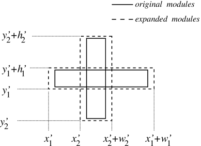
Figure 6: An impossible, crossing position for expanded modules.

Theorem 1

The expanded regions $m^{\prime}_{i},m^{\prime}_{j}\in M^{\prime}$ for two existing, disjoint modules $m_{i},m_{j}\in M$ cannot cross.

Proof: Every expanded module $m^{\prime}_{i}$ is a rectangle, described by four bounding coordinates: $x^{\prime}_{i}$, the position of its left edge; $x^{\prime}_{i}+w^{\prime}_{i}$, the position of its right edge; $y^{\prime}_{i}$, the position of its lower edge; $y^{\prime}_{i}+h^{\prime}_{i}$, the position of its upper edge. Now assume there are two expanded modules that cross, say, $m_{1}$ and $m_{2}$, and consider without loss of generality that $x^{\prime}_{1}<x^{\prime}_{2}$. Then crossing means that $x^{\prime}_{2}+w^{\prime}_{2}<x^{\prime}_{1}+w^{\prime}_{2}$, $y^{\prime}_{2}<y^{\prime}_{1}$, and $y^{\prime}_{1}+h^{\prime}_{1}<y^{\prime}_{2}+h^{\prime}_{2}$. But as all expanded modules arise from the original modules by moving their edges by the same amount for each coordinate direction, the same relative order must be valid for the original edges. This implies that the original modules cross, contradicting their disjointness.  $\Box$

Theorem 2

FindContourSegments finds $O(n)$ contour segments.

Proof: We will argue that the number of segments of the contour is at most the number of segments of all modules.

Consider the frontier $O_{i}=\{[b_{1},e_{1}],\ldots,[b_{o},e_{o}]\}$ of all open segments just before encountering event $L_{i}=(p_{i},t_{i},b_{i},e_{i})$.

Let us consider an $Open$ event $L_{i}$. Processing this event yields at most $|O_{i}|$ new contour segments. This is the case if and only if all elements $[b_{j},e_{j}]\in O_{i}$ are completely contained in $[b_{i},e_{i}]$ and do not overlap. But because no two modules can cross, all $Close$ events $L_{j^{\prime}}$ must occur before the $Close$ event $L_{i^{\prime}}$. Consequently the closing segments $[b_{j^{\prime}},e_{j^{\prime}}]$ do not contribute to the contour and in total the number of segments added is at most one.

Now let us consider a $Close$ event $L_{i}$. Arguing as above, we conclude that if $[b_{i},e_{i}]$ is totally contained in an element $[b_{j},e_{j}]\in O_{i}$, the total number of segments added to the contour is at most one.

In all other events at most one segment is added to the contour. As there are not more than $2n$ events in each cordinate direction, the number of contour segments parallel to each axis is at most $2n$. Thus, the number of contour segments is at most $4n$, i.e., linear in $n$.  $\Box$

2.4 Computational Complexity

Theorem 3

The complexity of FindContourSegments is $O(n\log n)$.

Proof: The algorithm CUR has a running time of $O(n\log n+s)$, where $s$ is the number of segments of the contour. As we have shown in Theorem 2, $s=O(n)$. Our modifications to CUR do not increase the running time by more than a constant factor. Thus the running time of FindContourSegments is $O(n\log n)$.  $\Box$

2.5 Lower Bound

Assuming a standard computational model, we can show that our FSM has optimal running time, by providing a matching lower bound:

Theorem 4

In the algebraic tree model of computation, there is a lower bound of $\Omega(n\log n)$ on the complexity of deciding the maximum size of a free rectangle between $n$ existing rectangles.

Proof: The claim is already true in one dimension, for $n$ existing unit intervals, with positions described by $n$ integers $a_{1},\ldots,a_{n}$. Determining a maximum free interval is precisely the problem Maximum Gap.

The Maximum Gap problem is the problem of determining the maximum gap between two consecutive numbers of a set $A=\{a_{1},a_{2},\ldots,a_{n}\}$ of $n$ numbers. Two elements of $A$ are called consecutive if they appear consecutively in the sequence obtained by sorting $A$. The running time of Maximum Gap is bounded from below by $\Omega(n\log n)$, as described in Chapter 6 of [15].  $\Box$

3 Routing-Conscious Placement

After describing how to find all feasible placements for a new module, we turn to finding an optimal placement, such that the weighted communication cost is minimized. As described in the introduction, an appropriate measure for this cost is the Manhattan distance between modules, weighted by the relative amount of communication. This can still be achieved in time $\Theta(n\log n)$, making use of local optimality properties, our FSM, and another application of plane sweep techniques.

3.1 Model

Given $F^{\prime}$ and $M^{\prime}$ as in Section 2, the objective of the placer is to find a point in free space that minimizes communication cost for the new module $m$.

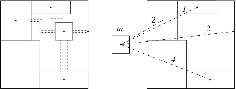
Figure 7: (Left) Physical chip with one module and its connectivity to other modules drawn by dotted lines (Right) Dotted lines with bandwidth attribute $b_{i}^{m}$ to denote required connectivity of module $m$ to other modules $i$.

In our routing-conscious approach we let the communication cost of an additional module $m$ depend on the distance to the centers of a subset of existing modules, which is measured in the Manhattan metric. We may also consider communication with the chip boundary as indicated in Figure 7. So we have to consider the set $C=\{(x_{1},y_{1}),\ldots,(x_{k},y_{k})\}$ of demand points for communication. Clearly, we may assume that the number $k$ of connections to be established with module $m$ is linear in $n$. A second factor in communication cost is the width $b^{m}_{i}$ of the communication path needed to create a routing unit between modules $i$ and $m$; this needs to be taken into account as a multiplicative factor. Thus, we get the objective function

$$\min\{c(x^{\prime}_{m},y^{\prime}_{m}):(x^{\prime}_{m},y^{\prime}_{m})\in F^{\prime}\setminus\bigcup_{m^{\prime}_{i}\in M^{\prime}}m^{\prime}_{i}\}$$

with

$$c(x,y)=\sum_{i=1}^{k}b^{m}_{i}\|(x_{i},y_{i})-(x,y)\|_{1}.$$

Because we are dealing with the Manhattan metric, this can be reformulated to

$$c(x,y)=c^{x}(x)+c^{y}(y)$$

with

$$c^{x}(x)=\sum_{i=1}^{k}b^{m}_{i}|x_{i}-x|,$$

and

$$c^{y}(y)=\sum_{i=1}^{k}b^{m}_{i}|y_{i}-y|.$$

If we would allow $$m^{\prime}$$ to be placed anywhere on the chip this can be reformulated to

$$\min\{c^{x}(x^{\prime}_{m}):x^{\prime}_{m}\in[{\frac{w_{m}}{2}},W\!-\!{\frac{w_{m}}{2}}]\}+$$

$$\min\{c^{y}(y^{\prime}_{m}):y^{\prime}_{m}\in[{\frac{h_{m}}{2}},H\!-\!{\frac{h_{m}}{2}}]\}.$$

As a consequence we can consider two separate minimization problems, one for each coordinate. If we ignore feasibility, both minima are attained in the respective weighted medians, so they can be computed in linear time [20]; as we already sort the coordinates for performing plane sweep, this running time is not critical, so we may as well use a trivial method. Note that only medians satisfy unconstrained local optimality, as the gradients for $$c^{x} c^{y}$$ and are simply

$$\nabla c^{x}(x)=\sum_{x_{i}<x}b^{m}_{i}-\sum_{x_{i}>x}b^{m}_{i},$$

the sum of the required bandwidths to the left minus the sum of the required bandwidths to the right and

$$\nabla c^{y}(y)=\sum_{y_{i}<y}b^{m}_{i}-\sum_{y_{i}>y}b^{m}_{i},$$

the sum of the required buswidths to the bottom minus the sum of the required buswidths to the top.

3.2 Local Optimality

As we have seen in the previous subsection the median is the globally optimal point if it is not in the occupied space. If it is in the occupied space there are only two other types of points where the global optimum could be located.

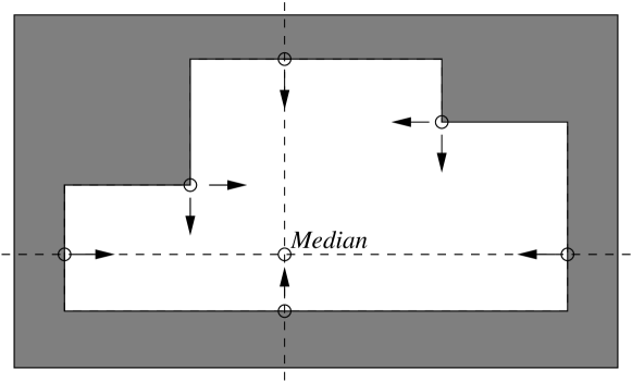
Figure 8: All potentially optimal points are marked by circles. As the median is located in the occupied space one of the other points must be optimal. The arrows show the directions in which the solution value would improve.

All points of one type can be found by intersecting the contour of the occupied space with the median axes $l_{x}=\{(x_{med},y):y\in[0,H]\}$ and $l_{y}=\{(x,y_{med}):x\in[0,W]\}$. In these points one of the gradients $\nabla c^{x}$ and $\nabla c^{y}$ vanishes. We cannot move in the direction of a better solution because that way is blocked by either a vertical or a horizontal segment of the contour.

The other type of points are some of the vertices of the contour. These points are the intersections of horizontal and vertical segments forming an interior angle of $\frac{\pi}{2}$ pointing in the direction of the median. In these points neither of the gradients vanishes. Either of the directions indicated by the gradient are blocked by contour segments.

By simply inspecting all the local optima one finds the global optimum. In the next subsection we describe how this can be done efficiently.

3.3 Algorithm for Global Optimality

The FSM described in the previous section computes the contour of the occupied space in $O(n\log n)$. A simple algorithm that finds the optimal point to place a new module $m$ would compute the median and check its feasibility; if the outcome is positive, we have found the optimum. Otherwise we need to check communication cost for all other possible local minima, i.e., for every vertex of the contour and every intersection point of the contour with one of the median axes. Let $L$ denote this set of points. Computing commuication cost for a single point takes $O(n)$, so evaluating all objective values in a brute-force manner would take $O(n^{2})$ time. However, by means of two more plane sweeps, we can achieve a complexity of $O(n\log n)$.

For this purpose, we observed that communication cost for the $x$- and $y$-coordinate of the contour segments can be computed separately, then add the precomputed values for every point of $L$. The crucial step is to use the fact that we only need to compute the communication cost for the leftmost $x$-coordinate and for the bottommost $y$-coordinate; the other values can be obtained by doing appropriate fast updates during the plane sweep. Below we give details of this step; for ease of presentation, we add the communcation points $C$ to $L$ — $L^{\prime}=L\cup C$ and only describe updates for $x$-coordinates.

First we sort (in time $O(n\log n)$) $L^{\prime}$ by increasing $x$-coordinate. Next we remove all points that are located on the same $x$-coordinate in $O(n)$ time. With the convention that $b^{m}_{i}=0$ if $(x_{i},y_{i})\in L\setminus C$ we compute the required bandwidth to the left and to the right of each point $i$ by $l_{i}=0$, $l_{i}=l_{i-1}+b^{m}_{i}$, $r_{|L^{\prime}|}=0$, and $r_{i}=r_{i+1}+b^{m}_{i}$. These values can be computed by a forward and a backward scan in $O(n)$ time. This yields the following recursive formula

$$c^{x}_{i+1}=c_{i}+(l_{i}-r_{i+1})(x_{i+1}-x_{i})$$

for computing communication cost for all $x$-coordinates in time linear in $n$.

As the lower bound from the previous section still applies, we get the following:

Theorem 5

A feasible position with minimum communication cost can be computed in time $\Theta(n\log n)$.

4 Experimental Results

		Running Time (ms)			Routing Cost			Rejection Rate
		RCP	NAO	KFF	RCP	NAO	KFF	RCP	NAO	KFF
Uniform	5-10%	173	197	204	1403	3641	9522	0%	0%	0%
Uniform	10-15%	162	208	194	1747	5490	14311	0%	1%	0%
Uniform	15-20%	160	172	158	2044	7250	19791	2%	5%	1%
Uniform	20-25%	156	181	161	1987	7061	20159	10%	12%	9%
Uniform	5-25%	168	224	215	1721	6741	21347	5%	8%	5%
Increasing	5-25%	196	252	243	1931	6914	21910	8%	14%	6%
Decreasing	25-5%	175	232	228	611	2311	11712	0%	3%	4%
Average		170	209	200	1635	5630	16965	3.6%	6.1%	3.6%

Table 1: Experimental results for the different benchmark instances. Overall running time, average routing cost for each module, and rejection rate are shown for the different algorithms. RCP denotes the algorithm described in this paper, NAO refers to the algorithm as described in [5] and KFF is the algorithm KAMER combined with First Fit as presented in [3]

The running time of our algorithm is not only good in theory, but also quite practical (as constants are small) and easy to implement. Here we show some results of our implementation. See Table 1 for an overview.

We randomly generated two different kinds of benchmark instances. All of the instances describe a scenario in which 100 modules have to be placed on an initially empty chip of size $80\times 120$. Each module stays on the chip until at least a certain number of new modules have been placed. Then it is removed from the chip. This number is different for each module and is randomly drawn from the interval $[4,100]$. Each of the modules needs to communicate with the border of the chip and with all the modules located on the chip. The buswidth is drawn for the interval $[0,10]$.

The instances differ in module size and distribution of the sizes. We have generated instances where all modules have roughly the same size (5-10%, 10-15%, 15-20%, and 20-25% of the chip size). These instances are called uniform since the sizes are distributed uniformly. We also have created instances where module sizes vary from 5 to 25% of the chip size. Here we consider three different kinds of distributions – uniform, increasing, and decreasing. In the increasing and decreasing case the modules are sorted by size.

Given these instances we benchmarked a g++ 3.2 compiled c++ implementation of our algorithm against the algorithms described in [5] and [3]. Shown in the first set of columns in the table is a comparison of average running times for 100 modules for each instance in milliseconds on a 2.53GHz Intel Pentium 4 PC running under the linux operating system. Remarkably, our algorithm on average has the fastest running time, even though it computes much better solutions. This illustrates the superiority of a plane-sweep apporach. Clearly, the difference in running times will increase for even larger instances.

The second set of columns compares the average routing cost per module. Routing costs are measured according to the weighted Manhattan distance, which reflects the fact that routing on the chip is done in an axis-parallel manner. Note that in [5], placement is done according to a weighted Euclidean distance, and optimization is only done heuristically. As a consequence, the objective values are markedly higher. [3] does not take routing cost into account and places by some bin-packing like heuristic trying to minimize rejection rate. This may result in modules being placed all over the chip, regardless of communication cost. As a result, communication cost is one order of magnitude higher than for our method.

As a matter of fairness, we give a third set of columns, comparing the average number of modules that had to be rejected due to lack of space on the chip, which is one of the objectives in [3]. Note that this rejection rate does not play any role during the course of our algorithm, nor is it considered in [5]. It is striking that nevertheless, the total number of rejected modules for our algorithm is precisely the same as for [3]. Again, our results dominate the ones for [5] by a clear margin.

In summary, our algorithm is faster except for case uniform15-20%, better and more robust against rejection than the method described in [5]. It is also faster, much better and as robust against rejection as the approach described in [3].

5 Conclusion

We have shown how to deal with two crucial issues supporting partial reconfigurability in reconfigurable computing. This raises hope of achieving further progress for even more complicated scenarios. One such aspect is to streamline our data structures and algorithms for repeated insertion or removal of modules. Some computational work can be saved, as sorting from scratch is no longer required. While this makes it relatively straightforward to lower the resulting complexity of dealing with $n$ changes in total time $O(n^{2})$, it remains an open challenge to decide whether a subquadratic complexity is possible, as no appropriate techniques for establishing quadratic lower bounds are known. However, it is conceivable that we may be facing a 3SUM-hard problem, which is the next best thing to an explicit lower bound. See [21] for techniques used for showing this for other geometric problems.

An even more interesting challenge arises by venturing from “routing-conscious” placement to “routing-optimal” placement: When routing among existing modules, we may have to consider them as obstacles for our paths. Thus, distances are not straight-line Manhattan distances, but geodesic Manhattan distances, i.e., given by shortest paths among obstacles. We believe that this type of problem can still be dealt with efficiently by using the techniques of Mitchell [22]. This has been done in [23] for an application to a routing-optimal placement problem for a continuum of demand points. For dynamic routing requests at runtime, principles that have been investigated include Dynamic Network on Chip (DyNoC) [24] and Honeycomb [25].

As our algorithm considers placing one module at a time, it is an interesting problem to consider the more complex task of placing the full set of modules at once. This is considered in [9] for the scenario of all processors being of the same size; even without existing modules and uniform routing cost, this turns out to be a tough problem, as noted in [8]. We hope to provide results on this scenario for modules of differing size and non-uniform routing cost in the near future.

Finally, it should be interesting to consider placement of modules as an online problem, where only limited information is available at each stage. Interesting scenarios require an appropriate modeling of the objective function considered, in particular for the tradeoff between computing cost, routing cost, and the cost of rejecting modules.

References

- [1] A. Ahmadinia, C. Bobda, S. Fekete, J. Teich, and J. van der Veen, “Optimal routing-conscious dynamic placement for reconfigurable computing,” in 14th International Conference on Field-Programmable Logic and Application, ser. Lecture Notes in Computer Science, vol. 3203. Springer-Verlag, 2004, pp. 847–851, available at http://arxiv.org/abs/cs.DS/0406035.
- [2] G. B. Wigley and D. A. Kearney, “The first real operating system for reconfigurable computers,” in Proceedings of 6th Australasian Computer Systems Architecture Conference (ACSAC 2001), 2001, pp. 130–137.
- [3] K. Bazargan, R. Kastner, and M. Sarrafzadeh, “Fast template placement for reconfigurable computing systems,” In IEEE Design and Test - Special Issue on Reconfigurable Computing, vol. January-March, pp. 68–83, 2000.
- [4] H. Walder, C. Steiger, and M. Platzner, “Fast Online Task Placement on FPGAs: Free Space Partitioning and 2D-Hashing,” in Proc. IPDPS-2003, Reconfigurable Architectures Workshop (RAW-2003), IEEE-CS Press. IEEE Computer Society, April 2003, p. 178.
- [5] A. Ahmadinia, C. Bobda, M. Bednara, and J. Teich, “A new approach for on-line placement on reconfigurable devices,” in Proc. IPDPS-2004, Reconfigurable Architectures Workshop (RAW-2004), IEEE-CS Press, 2004.
- [6] J. Tabero, J. Septién, H. Mecha, and D. Mozos, “A vertex-list approach to 2D HW multitasking management in RTR FPGAs,” in DCIS 2003, 2003, pp. 545–550.
- [7] ——, “A low fragmentation heuristic for task placement in 2D RTR HW management,” in 14th International Conference on Field-Programmable Logic and Application, ser. Lecture Notes in Computer Science, vol. 3203. Springer-Verlag, 2004, pp. 241–250.
- [8] R. M. Karp, A. C. McKellar, and C. K. Wong, “Near-optimal solutions to a 2-dimensional placement problem,” SIAM Journal on Computing, vol. 4, pp. 271–286, 1975.
- [9] M. A. Bender, D. P. Bunde, E. D. Demaine, S. P. Fekete, V. J. Leung, H. Meijer, and C. A. Phillips, “Communication-aware processor allocation for supercomputers,” in Proc. Workshop on Algorithms and Data Structures, ser. LNCS, F. Dehne, A. López-Ortiz, and J.-R. Sack, Eds., vol. 3608. Springer-Verlag, 2005, pp. 169–181.
- [10] S. Krumke, M. Marathe, H. Noltemeier, V. Radhakrishnan, S. Ravi, and D. Rosenkrantz, “Compact location problems,” Theor. Comp. Science, vol. 181, no. 2, pp. 379–404, 1997.
- [11] J. Mache and V. Lo, “Dispersal metrics for non-contiguous processor allocation,” University of Oregon, Technical Report CIS-TR-96-13, 1996.
- [12] ——, “The effects of dispersal on message-passing contention in processor allocation strategies,” in Proc. Third Joint Conference on Information Sciences, Sessions on Parallel and Distributed Processing, vol. 3, 1997, pp. 223–226.
- [13] R. H. Güting, “An optimal contour algorithm for iso-oriented rectangles,” J. Algorithms, vol. 5, pp. 303–326, 1984.
- [14] W. Lipski, Jr. and F. P. Preparata, “Finding the contour of a union of iso-oriented rectangles,” J. Algorithms, vol. 1, pp. 235–246, 1980, errata in 2(1981), 105; corrigendum in 3(1982), 301–302.
- [15] F. P. Preparata and M. I. Shamos, Computational Geometry: An Introduction. New York, NY: Springer-Verlag, 1985.
- [16] M. de Berg, M. van Kreveld, M. Overmars, and O. Schwarzkopf, Computational Geometry: Algorithms and Applications, 2nd ed. Berlin, Germany: Springer-Verlag, 2000.
- [17] J. L. Bentley, “Multidimensional binary search trees used for associative searching,” Commun. ACM, vol. 18, no. 9, pp. 509–517, 1975.
- [18] ——, “Solutions to Klee’s rectangle problems,” Carnegie-Mellon Univ., Pittsburgh, PA, Technical Report, 1977.
- [19] J. L. Bentley and D. Wood, “An optimal worst case algorithm for reporting intersections of rectangles,” IEEE Trans. Comput., vol. C-29, pp. 571–577, 1980.
- [20] M. Blum, R. W. Floyd, V. Pratt, R. L. Rivest, and R. E. Tarjan, “Linear time bounds for median computations,” in Proc. Fourth Annual ACM Symposium on Theory of Computing, 1972, pp. 119–124.
- [21] G. Barequet and S. Har-Peled, “Polygon containment and translational min-Hausdorff-distance between segment sets are 3SUM-hard,” Internat. J. Comput. Geom. Appl., vol. 11, pp. 465–474, 2001.
- [22] J. S. B. Mitchell, “An algorithmic approach to some problems in terrain navigation,” Artif. Intell., vol. 37, pp. 171–201, 1988.
- [23] S. P. Fekete, J. S. B. Mitchell, and K. Weinbrecht, “On the continuous Weber and -median problems,” in Proc. 16th Annu. ACM Sympos. Comput. Geom., 2000, pp. 70–79, full version to appear in Operations Research.
- [24] C. Bobda, M. Majer, A. Ahmadinia, D. Koch, and J. Teich, “A dynamic NoC approach for communication in reconfigurable devices,” in Proceedings of International Conference on Field-Programmable Logic and Applications (FPL), ser. Lecture Notes in Computer Science, vol. 3203, 2004, pp. 1032–1036.
- [25] A. Thomas and J. Becker, “Dynamic adaptive runtime routing techniques in multigrain reconfigurable hardware architectures,” in Proceedings of International Conference on Field-Programmable Logic and Applications (FPL), ser. Lecture Notes in Computer Science, vol. 3203. Springer, 2004, pp. 115–124.